New Method to Determine the Dynamic Fluid Flow Rate at the Gear Pump Outlet

Abstract

External gear pumps are among the most popular fluid power positive displacement pumps; however, they often suffer from excessive flow pulsation transmitted to the downstream circuit. To meet the increasing demand of quiet operation for modern fluid power systems, it is necessary to give a physically sound method of analyzing the operation of a volumetric pump. The analysis of the basic approach used by the majority of researchers for calculating the flow rate of a gear pump by E.M. Yudin is presented. The article presents a new method for analyzing the operation of volumetric pumps. The method is suitable for the pumps whose dynamic characteristics should be considered according to the model of an equivalent source of flow fluctuations by V.P. Shorin. The method is based on wave theory, the method of hydrodynamic analogies and the impedance method, where the pump is considered according to the model in lumped parameters. The method consists in determining the pressure pulsations at the pump output in bench systems with known dynamic characteristics and recalculating the pump flow rate in pulsations. Computational dynamic models of bench systems in lumped parameters are proposed for subsequent use in dynamic tests of pumps in the form of equivalent sources of fluid flow fluctuations. We give recommendations for the formation of test bench systems with a throttle, a cavity and a pipeline at the pump output. Using the example of an external gear pump with a working volume of 14 cm³/rev, the implementation of the proposed method is considered. The pump’s own pulsation characteristic of the flow rate in a bench system with an “infinitely long” pipeline along two harmonic components of the spectrum is determined, and a test of the method based on the method of determining the instantaneous flow rate by R.N. Starobinskiy is proposed. It is shown that, according to the proposed method and the method of R.N. Starobinskiy, the divergence of the amplitudes of flow pulsations does not exceed (5–10)%. The high degree of coincidence of the results confirms that the external gear pump in question should be considered according to the equivalent source of flow fluctuations model.

1. Introduction

Gear pumps are the most common devices for converting mechanical energy in machines and mechanisms into hydraulic energy of a fluid flow. Such a transformation has found wider application in various branches of technology since the beginning of the 20th century. For example, it is used in actuating hydraulics of mechanical handling machines, road construction equipment, hydraulic drives of machine tools and, of course, in fuel systems to create the necessary fuel supply pressure.

Hundreds of research, development, design and engineering studies have been devoted to the issues of ensuring the most efficient operation of pumps in terms of energy conversion efficiency, weight reduction, increasing reliability of operation and reducing the noise generated by pumps. The number of studies is still growing due to increasing requirements and technology level.

The first founders and researchers of the volumetric pump operation in the USSR were scientists such as T.M. Bashta, E.M. Yudin [1,2] and many others [3,4,5,6,7]. The papers of T.E. Beecham, W.E. Wilson, D. McCandlish, K. Foster, K.A. Edge, D.N. Johnston, M. Ivantysynova, A. Vacca, K. Manco, J. Strzyczek and V. Fiebig [8,9,10,11,12,13,14,15,16,17,18] are known in other countries.

As a result, by the end of the 20th century, the following developments were made:

• ₋ The theoretical performance of the gear pump (kinematic fluid supply) was determined. Such a supply is characterized by nonuniformity due to the cyclic supply of each gear tooth with mutual coverage of the opposite gear teeth [1,2,8,9];
• ₋ Hydraulic fluid leakage from the high-pressure cavity to the fluid inlet through gaps and surface roughness was determined [1,2,5,8,9,10];
• ₋ The effect of reverse hydraulic impact from the pump outlet manifold into the tooth/sub-plunger space was determined. The impact magnitude is determined by the pressure level in the outlet manifold, the dynamic properties of the outlet manifold, the volume of the tooth/sub-plunger space and the pressure level in the tooth cavity or under the plunger at the moment of juncture with the outlet pressure manifold [1,2,4];
• ₋ The level of pressure increase in the trapped volume at the moment when the gear teeth pass through the closure between the pump and suction lines was determined. This increase in pressure causes shock loads on the gear shafts, which leads to vibration of the gears and pump casing and the acoustic noise generated by the pump [1,2,8,11].

In experimental studies, scientists agree that the results of experimental studies are often contradictory and do not fully correspond to the results of theoretical studies [1,2,19,20,21,22]. For example, the author Yu.V. Kuleshkov [20], while analyzing the materials of the article [15], concluded that the degree of unevenness of the feed according to the numerical model of Casoli P. et al. not less than (3 … 5) times less than according to traditional ideas [2]. In the work of Chai H. et al. [22], according to the results of numerical simulation, it is stated that, for an internal gear pump, the variable component of the internal leakage is 80% of the total flow pulsation, and the geometric flow pulsation is only 20%, while experimental confirmation is not given, which means the relative reliability of the data only obtained. In the article [21], Vacca A. calculated that, while the gear pump of the external gearing is operating at 2000 rpm and 200 bar on a bench system with a restriction-termination circuit and with a volume-termination circuit, the pulsation caused by pressurization component of the ripple in the interdental chamber twice more than in a restriction-termination circuit. At the same time, the amplitude of flow fluctuations generated by the displacement process is practically unchanged in both bench systems. Thus, Vacca A. comes to the conclusion that two mechanisms for generating pulsations in the pump (kinematic component and a pressurization component) must be considered as independent sources of oscillations. Thus, in the articles under consideration, the issue of determining the own pulsation of the pump flow is not considered. Flow fluctuations resulting from the interaction between the pump and the connected system are determined. This leads to the differences in the obtained results and the impossibility of their objective and visual interpretation.

At the same time, none of the researchers has previously proposed or implemented a reliable approach explaining the physical nature of the pump dynamics (pressure and flow pulsations in the system after it) and calculation tools for this, which was confirmed by literature analyses and the conclusions of various authors [15,16,19,20,21,22,23].

Speaking about the CFD approach, the works by Yoon et al. [24] are important, as they perform the CFD analysis of the gear pump using the immersed solid method with commercial CFX software. Qi et al. [25] modeled the helical external gear pump using the Simerics MP+ commercial software. Castilla et al. published several studies on 3D CFD models for a gear pump developed based on the open-source OpenFOAM library [26,27]. The most significant works on dynamic lumped parameter models are represented by the contributions by Vacca and Guidetti [28], Mucchi et al. [29] and their subsequent works [30,31]. However, most of the mentioned modeling methods are still too complex for the pump analysis and take into account the hydrodynamics of the bench system.

This leads to this paper’s point, which is to propose an approach in order to determine the pump’s own pulsation flow rate and provide verification of the obtained results. The proposed approach is inspired by the works of G. Olson, V.P. Shorin, A.V. Artyukhov, Johnston D.N. and the early works of V.I. Sanchugov on the calculation of the pump’s own dynamic characteristics and the formation of special bench systems [6,13,32,33,34]. Thus, the pump is considered as a source of flow fluctuations in lumped parameters from the point of view of wave theory and the method of hydrodynamic analogies. The discussion focuses on the direct formation of the method, the proposed bench systems for determining the variable component of the pump flow rate and experimental verification based on the method for determining the instantaneous flow rate of R.N. Starobinskiy. Before that, the main drawbacks of the basic theory of gear pump feeding, disclosed in the works of E.M. Yudin and T.M. Bashta, based on the kinematic representation of displacement and stationary hydraulic formulas, are discussed.

The experimental studies results are implemented on a standard external gear pump, and the technical characteristics are presented in

Table 1. The gear pump specifications taken as reference in this approach.

Number of teeth	10	Diameter of tooth depressions (mm)	25.44
Coast pressure angle α (deg)	20	Center distance (mm)	33.16
Correction factor x	+0.0839	Axial length (mm)	27.6
Drive pressure angle αtw (deg)	22	Displacement (cc/rev)	14
Dividing diameter (mm)	32.5	Casing opening angle (deg)	47
Tooth tip diameter (mm)	39.94	Module (mm)	3.25

. The pump has identical gears with a symmetrical 10-teeth profile. However, the method proposed in this paper is suitable for the entire class of volumetric pumps, regardless of their design, speed range and operating pressures.

2. Analysis of Papers on the Gear Pump Operation

Initially, in the 1950s and 1960s, the study of pumps consisted in studying the changes of the pump cavity volumes in the suction and discharge areas. Based on the change in these volumes’ dq during the gear rotations, it was quite acceptable (and natural) in the early days of hydrodynamics to define the fluid supply as the time derivative of the volume change (dq/dt).

The result generally recognized by now is the representation of the kinematic supply in the form of a graph, which was called the flow pulsation (Figure 1).

Similar concepts are still in use today, for example, in the papers by A. Vacca and other authors [11,14,16,17,21,22,26,35] (Figure 2 and Figure 3).

However, the presented graphs (Figure 1, Figure 2 and Figure 3), named as “supply” or “flow rate”, are different. They were obtained based on the analysis of the change in the volume of the pump discharge cavities, limited by the involute profile of the meshing gears having a certain thickness. They do not describe the change in fluid supply but the rate of volume change for the discharge cavity. This, despite the coincidence of dimensions, is not the same thing at all.

Indeed, in the first papers of the 1950s and 1960s, the analysis of the pump operation was based not on a change in the fluid supply but on a change in the volume of the pump discharge cavity, which takes into account the ring gear width, cyclic frequency, engagement factor and other parameters that give very accurate results compared to experimental data. At the same time, E.M. Yudin [2] gives the following formula for calculating the theoretical supply:

$${\mathrm{Q}}_{\mathrm{th}}=2{\mathsf{\pi }\mathrm{b}}_{\mathrm{w}}\mathsf{\omega }\left({\mathrm{R}}_{\mathrm{e}}^2-{\mathrm{r}}^2-\mathrm{k}\frac{{\mathrm{t}}_0{}^2}{12}\right),$$

(1)

where

b_w—ring gear width (m),

ω—rotary cyclic frequency (rad/s),

R_e—circle radius of gear head (m),

r—pitch circle radius (m),

k—coefficient depending on the engagement factor and

t₀—base pitch (m).

This gives an error during the experimental calculation of performance of 1.4%. The same book contains a number of similar formulas for uncorrected and corrected gears with different profile displacements and pressure angles. A similar formula is presented in the manual [36] of the Rexroth Bosch Group:

$${\mathrm{Q}}_{\mathrm{th}}=\mathrm{q}·\mathsf{\omega }·{\mathsf{\eta }}_{\mathrm{v}},$$

(2)

where $\mathrm{q}$—pump volume displaced per revolution (m³/rev) and ${\mathsf{\eta }}_{\mathrm{v}}$—pump volumetric efficiency (%).

All these formulas, which slightly differ from each other in final results, determine the volume change $\mathrm{dq}$, erroneously called the pump supply flow, which is calculated by the change rate for the volume of the cavity displaced by the contacting tooth profiles of the meshing gears over an infinitesimal time interval $\mathrm{dt}$ [2]. This volume is defined as the product of the area between the moving tooth flanks and the tooth width:

$$\mathrm{dq}={\mathrm{b}}_{\mathrm{w}}\left({\mathrm{Re}}^2-{\mathrm{z}}^2-{\mathrm{x}}^2\right)\mathsf{\omega }\mathrm{dt},$$

(3)

where z—number of teeth, x—distance from the engagement point to the pole (m) and $\mathrm{dt}$—infinitesimal time interval (s).

These representations of the kinematic flow rate are erroneous for the following reasons:

• The founders of the gear pump theory suggested the wrong hypothesis that the change rate of the displaced volume (with the dimension of the flow rate) is the fluid flow rate at the pump outlet.
• The flow rate drops instantly at the engagement point for the second pair of teeth. This contradicts the energy conservation law and the law of fluid flow continuity because the fluid flow has two values (of the flow rate and, consequently, pressure) at the same moment in time.
• Presence of points where the flow rate direction changes abruptly (marked with red circles), which means that infinite forces are applied to the fluid flow. It is impossible according to the energy conservation law and, in particular, it contradicts the fluid flow continuity equation.
• The shown curves, constructed by calculation, are valid for the quasi-stationary (steady-state) regime of the fluid flow without taking the capacitive load, inertia of the fluid and the unsteadiness of the active resistance into account.
• The uneven supply is a source of high-frequency fluid fluctuations, which cannot be disregarded (Figure 4). At a pump speed of 3000 rpm and taking the number of teeth on the gears into account, the oscillation frequency from the first to the third harmonic is (500–2000) Hz. Hence, the pump operation is essentially a fast-acting and dynamic process.
• In addition, the processes of kinematic flow rate and reverse hydraulic impact, as well as the work of a choked volume, have a different nature. Therefore, there is no point in discussion about the liquid kinematic flow rate determined according to the laws and formulas of hydrostatics.

In reality, the fluctuations in pressure and flow rate of volumetric pumps have a polyharmonic nature, as evidenced by numerous experiments [12,37,38,39].

Furthermore, the processes of geometric supply and the work of a choked volume have a different nature. Therefore, there is no point as well in having a discussion about the geometric fluid supply determined by the laws and formulas of hydrostatics.

For these reasons, there are no results of physical experiments to determine the dynamic flow rate of the liquid at the pump outlet not only in the early studies by Bashta T.M., Yudin E.M. and Prokofiev V.N., but also in the modern studies by Shakhmatov E.V., Vacca A. and Rundo M. According to the modern literature and technical documentation (industry and state standards), it is fully sufficient to use such characteristics as the average pump performance in terms of fluid flow rate, generated pressure and efficiency during preliminary pump selection.

The calculated data on pulsating fluid flow given in numerous works and obtained using mathematical models show only the imperfection of the used models [9,11,14,17,22,35,40], created under a number of assumptions, where the main points are as follows:

-

The pump is accepted as a source of flow fluctuations by default;

-

The pressure at the inlet and outlet of the pump is accepted constantly;

-

The flow of the working fluid in the throttling elements is laminar;

-

The working fluid is incompressible;

-

Gear teeth are absolutely rigid;

-

Some of coefficients are determined experimentally under the assumption of internal pump flow’s quasi-stationarity;

-

The errors of the involute profile and the gear teeth division are negligible.

On the other hand, it should be noted that, with the current state-of-the-art methods, we do not have small-sized high-frequency liquid flow rate sensors that allow for direct measurements of this flow. The only option to determine the pump operation parameters under these conditions is to measure the pressure pulsations at the pump outlet in a system with known dynamic characteristics and then convert them into flow pulsations [37,38,39].

Therefore, if there are higher harmonics in the oscillation spectrum, then the maximum dimensions of the flow paths must reach 60–70 mm in order to fulfill the lumped model condition. Theoretical calculation and experimental methods can be used to evaluate the characteristics of a positive displacement pump.

Calculation methods should take into account the physical processes of fluid flow and the geometrical parameters of the pump design (geometric properties of gears, end and radial clearances between the pump rotor and stator, location and dimensions of pressure-relief slots and grooves), density and viscosity of the hydraulic fluid, pump speed, fluid compressibility in the pump cavities and fluid inertia in the channels of the flow path. For this purpose, simulation software packages can be used, for example, MATLAB-Simulink, Mathcad and other programs [41,42].

For the mathematical description of the pump dynamic characteristics, it is worthwhile to use the method of equivalent oscillation sources, first proposed by L. Thévenin and E. Norton [43,44] and developed by V.P. Shorin [6].

At the same time, V.P. Shorin [6] proposed to determine the characteristics of the oscillation sources according to the diagram of equivalent oscillation source (Figure 5).

The models presented in Figure 5 show that the characteristics of sources are determined by the performance of ideal sources and their internal impedance.

An ideal source of fluid flow fluctuations is a source with infinite internal impedance, in which fluid flow fluctuations do not depend on the dynamic characteristics of the connected systems.

In an electrical network, an alkaline electric battery can be roughly considered as such a source.

Real oscillation sources have finite internal impedance and limited power. Their characteristics are determined more precisely by the diagrams of equivalent oscillation sources (Figure 5). The values of the oscillatory performance, as well as their internal impedances, are derived from the design study, the properties of the hydraulic fluid and the connected hydraulic system. Experimental studies of the pump characteristics can be carried out taking into account the following circumstance.

In order to determine the pump characteristics, it is required to measure the oscillation components of pressure and flow rate of the fluid. When measuring the oscillating pressure, researchers do not encounter any particular difficulties. Nevertheless, there are no small-sized high-frequency liquid flow sensors in production. Therefore, the measurement of fluid flow rate has to be performed by indirect methods for measuring pressure in systems with a known impedance. To do this, it is necessary to place special bench systems at the pump outlet. In this case, the main task when choosing a bench system is to provide system parameters under which the best conditions for high measurement accuracy are realized. The choice of the connected system parameters must be carried out when the impedance changes in the range from −∞ to +∞.

Figure 6 shows:

(a)

A diagram of an ideal source of fluid flow fluctuations with an attached hydraulic system;

(b)

A graph of variance in the pressure fluctuation amplitude at the pump outlet ${\mathrm{A}}_{\mathrm{P}}$, taking active pressure losses ${\mathrm{ReZ}}_{\mathrm{b}.\mathrm{s}.}$ in the bench system into account;

(c)

Graphs of the phase shift of fluctuations of pressure and flow rate in the system.

The shape of curve shows that the amplitudes and phases of the pulsating pressure vary over a wide range due to changes in the dynamic properties of the bench system at a constant amplitude of source flow rate oscillations.

In the work of V.P. Shorin [6] bench systems are considered to be idealized objects with purely capacitive, inertial or active properties. Such systems are required to reflect the basic properties of the object, forming a boundary condition for calculating the fluid oscillation damper. His follower V.I. Sanchugov developed bench systems with the required nature and magnitude of the load impedance for solving the problems of gas-hydraulic flow cleaning and non-flow units [45] and solved the problem of determining the length of the pipeline that implements non-reflective resistance with a given degree of accuracy [34]. Later in the work of [46], the research group of Samara University made the first attempt to use a bench system with a damper with a constant active resistance equal to the wave resistance of the pipe behind the pump (${\mathrm{Z}}_{\mathrm{dam}}={\mathrm{Z}}_{\mathrm{b}.\mathrm{s}.}=\frac{\mathsf{\rho }\mathrm{a}}{\mathrm{S}}$, where ρ is the density of the working medium, a is the wave propagation velocity in the working environment and S is the cross-sectional area of the pipeline), to determine the pulsating flow behind the gear pump of external engagement and verification with a mathematical model of flow pulsations.

The work of R.N. Starobinskiy (1969) [47] presents a method for determining the instantaneous fluid flow in the middle of a “short” pipeline (Figure 7) by measuring the pressure drop at the ends of a smooth cylindrical dimensional pipeline and converting it into instantaneous fluid flow according to the formula:

$$\mathrm{g}\left(\mathrm{t}\right)=\frac{\Delta \mathrm{p}\left(\mathrm{t}\right)}{\left|{\mathrm{Z}}_{\mathrm{s}.\mathrm{p}.}\right|},$$

(4)

where

$\Delta \mathrm{p}$ is the difference of the instantaneous pressure values at the ends of the “short” pipeline for time $\mathrm{t}$ $\Delta \mathrm{p}={\mathrm{p}}_1-{\mathrm{p}}_2$;

${\mathrm{p}}_1,{\mathrm{p}}_2$ are the instantaneous pressure values at the beginning and end of the measuring pipeline, respectively;

${\mathrm{Z}}_{\mathrm{p}}$ is the impedance of the “short” pipeline ${\mathrm{Z}}_{\mathrm{s}.\mathrm{p}.}=\mathrm{j}2\mathsf{\pi }\mathrm{f}\frac{{\mathsf{\rho }\mathrm{l}}_{\mathrm{s}.\mathrm{p}.}}{\mathrm{S}}$;

$\mathrm{f}$ is the cyclic oscillation frequency;

$\mathrm{j}$ is an imaginary unit $(\mathrm{j}=\sqrt{-1}$);

${\mathrm{l}}_{\mathrm{s}.\mathrm{p}.}$ is the length of the “short” pipeline (limited by the condition of the lumped parameters ${\mathrm{l}}_{\mathrm{s}.\mathrm{p}.}\le \frac{\mathsf{\lambda }}{6}$);

$\mathsf{\lambda }$ is the wavelength $\mathsf{\lambda }=\frac{\mathrm{a}}{\mathrm{f}}$.

While using spectral analysis methods, for example, the Fourier series [48], the amplitude of the fluid flow ${\mathrm{A}}_{\mathrm{qk}}$ in the middle of the “short” pipeline for the k-th harmonic component is determined by the formula:

$${\mathrm{A}}_{\mathrm{qk}}\left(\mathrm{f}\right)=\frac{{\mathrm{A}}_{\Delta \mathrm{pk}}\left(\mathrm{f}\right)}{\left|{\mathrm{Z}}_{\mathrm{s}.\mathrm{p}.\mathrm{k}}\left(\mathrm{f}\right)\right|}$$

(5)

where ${\mathrm{A}}_{\Delta \mathrm{pk}}$ is the pressure amplitude difference at the ends of the “short” pipeline for the harmonic component.

Later, the “short” pipeline method was tested in the common rail (CR) fuel injection system. The prototypal flowmeter was installed at the delivery section of a CR volumetric pump in order to investigate the flow rate ripple. A. Ferrari took into account the active resistance component $\mathrm{R}$, which determines friction losses, when calculating the pipeline impedance [37,38]:

$${\mathrm{Z}}_{\mathrm{s}.\mathrm{p}.}=\mathrm{R}+\mathrm{j}2\mathsf{\pi }\mathrm{f}\frac{{\mathsf{\rho }\mathrm{l}}_{\mathrm{s}.\mathrm{p}.}}{\mathrm{S}},$$

(6)

A. Ferrari also verified the mathematical model using a “short” pipeline. A good agreement was found between the flowmeter rates and the theoretical predictions calculated with the developed A. Ferrari model.

Thus, the method of R.N. Starobinskiy makes it possible to determine the variable component of the flow rate in the middle of a dimensional “short” pipeline without directly determining the phase shift between ${\mathrm{p}}_1$ and ${\mathrm{p}}_2$. Such a measuring pipeline has no installation location limits in the bench system and is a reliable verification device.

The paper carried out the analysis of scientific articles of various scientific research groups on the work of gear pumps, generated pulsations and methods of their calculation. The purpose of the article is to offer a physically based approach to determine the pump’s own pulsation flow rate, to ensure verification of the obtained characteristics.

3. The Proposed Approach to the Analysis of Gear Pumps

In contrast to a number of other approaches that allow for calculating the variable component of pump flow according to mathematical models with various assumptions (incompressibility of the working fluid, absolute rigidity of pump elements, etc.), the authors propose to determine the variable component of pump flow directly in bench systems by the method described below. The proposed method resolves the contradictions formed from the middle of XX century, related to the physical model lack, a theoretical basis for describing the pump’s own pulsation performance and testing tools.

The method is formed at the junction of the hydrodynamic analogies method [32], the impedance method and spectral analysis methods [48]. The oscillation analysis is based on the wave equation solution for a plane wave.

The fluid flow in this case is determined by two components—pressure and flow rate—connected by impedance. Since the method is based on the wave theory of describing the liquid flow [49], the variable components of the flow rate g and pressure p are determined by the amplitude A, frequency ω and the initial phase φ on each harmonic component of the spectrum.

Hydrodynamic impedance is a generalized concept of resistance, or the ratio of pulsating pressure and pulsating flow in a complex form of representation:

$$\mathrm{Z}=\frac{\mathrm{p}}{\mathrm{q}},$$

(7)

where

$\mathrm{Z}$ is the complex resistance ($\mathrm{Z}=\left|\mathrm{Z}\right|{\mathrm{e}}^{\mathrm{j}\left({\mathsf{\phi }}_{\mathrm{p}}-{\mathsf{\phi }}_{\mathrm{q}}\right)}$);

$\mathrm{p}, \mathrm{q}$ are the variable component of pressure ($\mathrm{p}={\mathrm{A}}_{\mathrm{p}}{\mathrm{e}}^{\mathrm{j}(2\mathsf{\pi }\mathrm{ft}+{\mathsf{\phi }}_{\mathrm{p}})}$) and the flow rate ($\mathrm{q}={\mathrm{A}}_{\mathrm{q}}{\mathrm{e}}^{\mathrm{j}(2\mathsf{\pi }\mathrm{ft}+{\mathsf{\phi }}_{\mathrm{q}})}$), respectively;

${\mathrm{A}}_{\mathrm{p}},{ \mathrm{A}}_{\mathrm{q}}$ are the amplitude of pressure and flow pulsations, respectively;

${\mathsf{\phi }}_{\mathrm{p}},{ \mathsf{\phi }}_{\mathrm{q}}$ are the arguments of the variable component of pressure and flow, respectively.

Since the flow pulsations amplitude interests, the phase components ${\mathsf{\phi }}_{\mathrm{p}},{ \mathsf{\phi }}_{\mathrm{q}}$ were not taken into account.

A test scheme was used for determining the pulsating flow rate behind a pump operating on a bench system with dynamic characteristics in the impedance form ${\mathrm{Z}}_{\mathrm{b}.\mathrm{s}.}$. The schematic diagram of the tests is presented in Figure 8. The diagram shows the pump as a source of flow fluctuations with an average flow component ${\mathrm{Q}}_0$, a variable flow component ${\mathrm{q}}_{\mathrm{s}}$ and an impedance ${\mathrm{Z}}_{\mathrm{s}}$.

If the pump is an independent source of flow fluctuations, it has one amplitude-frequency characteristic (frequency response) of the flow in any bench systems, i.e., the frequency response does not depend on the dynamic properties of the bench system (frequency, geometry of the flow part of the system and the properties of the working medium).

The method consists in experimentally determining the amplitudes of pressure pulsations behind a pump interacting with a bench system; its impedance ${\mathrm{Z}}_{\mathrm{b}.\mathrm{s}.}$ is known in advance. Further, the processed pressure-frequency response using the impedance of the bench system ${\mathrm{Z}}_{\mathrm{b}.\mathrm{s}.}$ is recalculated into the flow-frequency response. Verification of the method should be carried out using the “short” pipeline of R.N. Starobinskiy, located directly behind the pump at a minimum distance.

The new method differs from the previous ones in that special bench systems are proposed to determine the variable component of the pump flow, taking into account the design of the flow part of the bench systems as connecting fittings, adapters and internal channels of the units. The calculated flow pulsations can be verified. As a result, the proposed method allows for the following:

-

To form special bench systems based on the throttle, cavity and pipeline with previously known dynamic characteristics;

-

To expand the possibilities of forming bench systems in lumped parameters in a wide range of dynamic loads from inertial to capacitive nature;

-

To check the calculated variable component of the flow rate using the “short” pipeline of R.N. Starobinskiy.

4. Models’ Creation, Calculation of Characteristics, Design and Manufacture of Special Systems at the Liquid Output from the Pump with Known Characteristics

Let us consider the basic options for bench systems at the outlet when testing pumps. In lumped parameters, the bench system should implement the following:

(1)

Active flow-dependent load;

(2)

Inertial load;

(3)

Capacitive load.

In distributed parameters, the bench system can be made in the form of an extended cylindrical pipeline that implements an active frequency-independent non-reflective load.

All operations and parametric analysis models of special bench systems are performed in Microsoft Excel.

4.1. Active Load Implementation

In order to implement an active bench load, you should place the throttle with active resistance at the pump outlet, providing the specified pump-operating mode for pressure and fluid flow. In this case, the further bench system can be ignored, since its properties are not able to affect the dynamic process of fluid fluctuations behind the pump with a significant pressure drop on the throttle. Moreover, in practice, it is not always possible to install the throttle directly behind the pump, so you have to use an additional connecting pipeline and consider its inertial properties as well as the length of the connecting fittings and penetrators in the pump, fuel line and throttle.

A throttle at the liquid outlet from the pump realizes the active load; the diagram shown in Figure 9 illustrates it.

The calculated hydrodynamic model shown in Figure 10 corresponds to the bench system and includes a pump as a source of constant fluid flow ${ \mathrm{Q}}_0$, a source of pulsating fluid flow with amplitude ${\mathrm{A}}_{\mathrm{q}}$, impedance ${\mathrm{Z}}_{\mathrm{S}}$ and an attached hydraulics. The bench system includes the following.

An active resistance ${\mathrm{Z}}_{\mathrm{thr}}$ realized by the throttle [6] (Figure 10) is calculated by the formula:

$${\mathrm{Z}}_{\mathrm{thr}}=\frac{\Delta {\mathrm{P}}_0}{{\mathrm{Q}}_0},$$

(8)

where

$\Delta {\mathrm{P}}_0$ is the pressure drop on the throttle ($\Delta {\mathrm{P}}_0={\mathrm{P}}_2-{\mathrm{P}}_1$),

${\mathrm{P}}_2$ is the average pressure in the line in front of the throttle,

${\mathrm{P}}_1$ is the average pressure in the line behind the throttle and

${\mathrm{Q}}_0$ is the average flow rate in the throttle.

The impedance of the bench system in the form of an active resistance realized by a throttle with a different cross-sectional area (${\mathrm{F}}_1<{\mathrm{F}}_2<{\mathrm{F}}_3$) is shown in Figure 11.

The throttle impedance has a linear dependence on the average flow rate in the ${\mathrm{Q}}_0$ system.

Therefore, the throttle impedance equation in the coordinates “the real part of the impedance is the flow rate” looks like the following:

$${\mathrm{Z}}_{\mathrm{thr}}=\frac{{\mathrm{Z}}_{\mathrm{thr}}{}_0}{{\mathrm{Q}}_0}{\mathrm{Q}}_{\mathrm{i}}=\mathrm{tg}\mathsf{\alpha }·{\mathrm{Q}}_{\mathrm{i}},$$

(9)

where ${\mathrm{Z}}_{\mathrm{thr}}{}_0$ is the real part of the impedance at a stationary flow rate ${\mathrm{Q}}_0$, $\mathsf{\alpha }$ is the angular coefficient of the straight line slope for the impedance change in flow rate and ${\mathrm{Q}}_{\mathrm{i}}$ is the current value of the fluid flow.

According to the calculations:

-

The fluid flow rate dependence of the throttle impedance is described by the equation of the straight line;

-

While decreasing in the area of the throttle passage section (${\mathrm{F}}_1>{\mathrm{F}}_2>{\mathrm{F}}_3$), the impedance of the throttle ${\mathrm{Z}}_{\mathrm{thr}}$ increases.

Considering the connecting pipeline ${\mathrm{l}}_{\mathsf{\Sigma }}$ long, including the connecting line, fittings and internal channels in the pump and throttle, whose inertial properties are necessary to be taken into account, the impedance of the throttle as an active-inertial bench system has the following form:

$${\mathrm{Z}}_{\mathrm{b}.\mathrm{s}.}\left({\mathrm{Q}}_0,\mathrm{f}\right)={\mathrm{Z}}_{\mathrm{thr}}\left({\mathrm{Q}}_0\right)+{\mathrm{ReZ}}_{\mathrm{pl}}\left({\mathrm{Q}}_0\right)+{\mathrm{jImZ}}_{\mathrm{b}.\mathrm{s}.}\left({\mathrm{f}}_{\mathrm{k}}\right),$$

(10)

where

${\mathrm{ReZ}}_{\mathrm{pl}}\left({\mathrm{Q}}_0\right)$ is the real part of the impedance of the pipeline, including the connecting line, fittings and internal channels in the pump and throttle;

${\mathrm{ImZ}}_{\mathrm{b}.\mathrm{s}.}$ is the inertial impedance of the bench system (${\mathrm{ImZ}}_{\mathrm{thr}}=2{\mathsf{\pi }\mathrm{f}}_{\mathrm{k}}\frac{{\mathsf{\rho }\mathrm{l}}_{\mathsf{\Sigma }}}{{\mathrm{S}}_{\mathrm{thr}}}$);

${\mathrm{f}}_{\mathrm{k}}$ is the frequency of the $\mathrm{k}$-th harmonics behind the pump;

$\mathrm{k}$ is the harmonics number;

${\mathrm{l}}_{\mathsf{\Sigma }}$ is the pipeline length, including the length of the line 6, connecting fittings 5 and 7 and internal channels of the pump and throttle (not shown in Figure 7);

${\mathrm{S}}_{\mathrm{pl} }$ is the cross-sectional area of the pipeline;

$\mathrm{j}$ is an imaginary unit ($\mathrm{j}=\sqrt{-1}$).

The bench system impedance with a throttle at the pump outlet has the following form:

$$\left|{\mathrm{Z}}_{\mathrm{b}.\mathrm{s}.}\right|=\sqrt{{({\mathrm{Z}}_{\mathrm{thr}}\left({\mathrm{Q}}_0\right)+{\mathrm{ReZ}}_{\mathrm{pl}}\left({\mathrm{Q}}_0\right))}^2+{\left(2{\mathsf{\pi }\mathrm{f}}_{\mathrm{k}}\frac{{\mathsf{\rho }\mathrm{l}}_{\mathsf{\Sigma }}}{{\mathrm{S}}_{\mathrm{pl}}}\right)}^2},$$

(11)

$${\mathsf{\phi }}_{\mathrm{b}.\mathrm{s}.}=\mathrm{arctg}\left[\frac{2{\mathsf{\pi }\mathrm{f}}_{\mathrm{k}}\frac{{\mathsf{\rho }\mathrm{l}}_{\mathsf{\Sigma }}}{{\mathrm{S}}_{\mathrm{pl}}}}{{\mathrm{Z}}_{\mathrm{thr}}\left({\mathrm{Q}}_0\right)+{\mathrm{ReZ}}_{\mathrm{pl}}\left({\mathrm{Q}}_0\right)}\right]+2\mathsf{\pi }\mathrm{n}, \mathrm{where} \mathrm{n}=1,2,3\dots \mathrm{m},$$

(12)

where $\mathrm{m}$ is an integer.

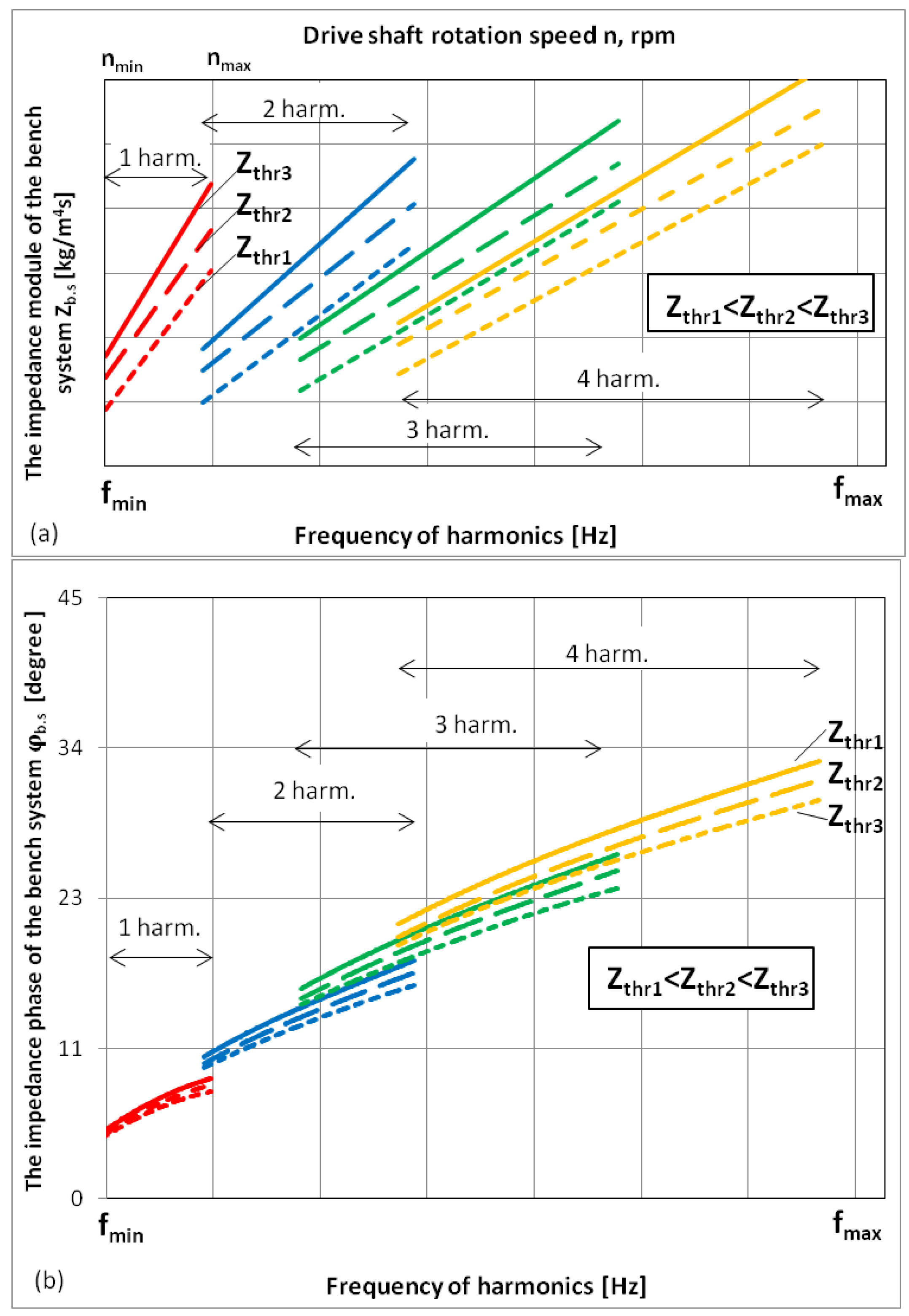
Parametric analysis of the bench system impedance ${\mathrm{Z}}_{\mathrm{b}.\mathrm{s}.}\left(\mathrm{f}\right)$ when the throttle impedance changes ${\mathrm{Z}}_{\mathrm{thr}1}<{\mathrm{Z}}_{\mathrm{thr}2}<{\mathrm{Z}}_{\mathrm{thr}3}$ for the four harmonic components of the oscillation spectrum is shown in Figure 12.

Analysis of Figure 12:

-

The impedance module of the bench system has a linear character and depends on the resistance of the throttle ${\mathrm{Z}}_{\mathrm{thr} }$ and the inertial impedance of the pipeline ${\mathrm{ImZ}}_{\mathrm{pl}}$;

-

The phase of the impedance of the bench system decreases with increasing throttle impedance (at ${\mathrm{Z}}_{\mathrm{thr}1}<{\mathrm{Z}}_{\mathrm{thr}2}<{\mathrm{Z}}_{\mathrm{thr}3}$);

-

In the low-frequency region, the impedance of the bench system is mainly characterized by the impedance of the throttle ${\mathrm{Z}}_{\mathrm{thr} }$; in the high-frequency area, the impedance of the bench system is mainly characterized by the connecting pipeline impedance ${ \mathrm{ImZ}}_{\mathrm{pl}}$.

4.2. Implementation of Inertial Load

To realize the inertial impedance in the lumped parameters at the pump outlet, it is necessary to place a segment of a straight cylindrical pipeline ${\mathrm{l}}_2$ long and ${\mathrm{D}}_{\mathrm{pl} }$ across, a significant cavity volume ${\mathrm{V}}_{\mathrm{c}}$ and a load throttle with an impedance ${\mathrm{Z}}_{\mathrm{thr}}$ (Figure 13).

In this case, the pipeline at the pump outlet together with the fittings form an element of inertia. The cavity at the pump outlet implements the acoustically open end of the pipeline, and the throttle provides a static mode of operation of the pump.

Figure 14 presents the calculation model of such system. Since the cavity of the “infinite” volume 3 is characterized by a small impedance modulus, the model does not indicate the cavity impedance in Figure 14. That is why the throttle impedance is not taken into account while calculating dynamic processes.

Proposed model features:

• All lines and fittings (2,6,7) should be considered as elements described by equations in lumped parameters at the maximum frequencies of the oscillation spectrum for pump 1.
• The implementation of the inertial impedance at the pump 1 output assumes an acoustically open output from the line 2. The output is provided by installing a significant volume of cavity 3 into the system, the pressure fluctuations of which can be neglected (${\mathrm{A}}_{\mathrm{p}}=0$).
• When performing calculations, the total length of the pipeline is determined as ${\mathrm{l}}_{\mathsf{\Sigma }}={\mathrm{l}}_6+{\mathrm{l}}_2+{\mathrm{l}}_7$ with a corresponding increase in hydraulic resistance ${\mathrm{ReZ}}_{\mathrm{pl}}=\mathrm{R}={\mathrm{R}}_6+{\mathrm{R}}_2+{\mathrm{R}}_7$ and inertia $\mathrm{L}=\frac{\mathsf{\rho }}{{\mathrm{S}}_{\mathrm{pl}}}\left({\mathrm{l}}_6+{\mathrm{l}}_2+{\mathrm{l}}_7\right)=\frac{{\mathsf{\rho }\mathrm{l}}_{\mathsf{\Sigma }}}{{\mathrm{S}}_{\mathrm{pl}}}$.

The input impedance of the bench system implementing the inertial pump load is defined as follows:

$${\mathrm{Z}}_{\mathrm{b}.\mathrm{s}.}\left({\mathrm{Q}}_0,{\mathrm{f}}_{\mathrm{k}}\right)={\mathrm{ReZ}}_{\mathrm{pl}}\left({\mathrm{Q}}_0\right)+{\mathrm{jImZ}}_{\mathrm{pl}}\left({\mathrm{f}}_{\mathrm{k}}\right),$$

(13)

where

${\mathrm{ReZ}}_{\mathrm{pl}}$ is the real part of the pipeline impedance determined by the well-known stationary hydraulics formulas [6,9];

${\mathrm{ImZ}}_{\mathrm{pl}}$ is the inertial impedance of the bench system ${\mathrm{ImZ}}_{\mathrm{pl}}=2{\mathsf{\pi }\mathrm{f}}_{\mathrm{k}}\frac{{\mathsf{\rho }\mathrm{l}}_{\mathsf{\Sigma }}}{{\mathrm{S}}_{\mathrm{pl}}}$;

${\mathrm{l}}_{\mathsf{\Sigma }}$ is the length of the pipeline, including the length of line 2, connecting fittings 6 and 7 and the internal channels of the pump and the cavity (not shown in Figure 13);

${\mathrm{S}}_{\mathrm{pl}}$ is the cross-sectional area of the pipeline length ${\mathrm{l}}_{\mathsf{\Sigma }}$;

$\mathrm{j}$ is an imaginary unit ($\mathrm{j}=\sqrt{-1}$).

Thus, according the connecting fittings 6 and 7 at the pump outlet 1, the calculated hydrodynamic model of the bench system implementing the “inertial” load will take form as in Figure 15.

To project according to the proposed calculation model, it is necessary to determine the type of fluid flow using the Reynolds criterion:

$$\mathrm{Re}=\frac{4{\mathrm{Q}}_{\max }}{{\mathsf{\pi }\mathsf{\nu }\mathrm{D}}_{\mathrm{pl}}},$$

(14)

The actual part of the pipeline impedance is calculated as:

$${\mathrm{ReZ}}_{\mathrm{pl}}=\frac{\Delta {\mathrm{P}}_{\mathrm{pl}}}{\mathrm{Q}}=\frac{\Delta {\mathrm{P}}_{\mathrm{lam}}+\Delta {\mathrm{P}}_{\mathrm{turb}}+\Delta {\mathrm{P}}_{\ln }}{\mathrm{Q}}={\mathrm{ReZ}}_{\mathrm{lam}}+{\mathrm{ReZ}}_{\mathrm{turb}}+{\mathrm{ReZ}}_{\ln },$$

(15)

Impedance of the connecting pipeline ${\mathrm{ImZ}}_{\mathrm{pl}}$ is considered in the previous section.

The bench system impedance (the modulus and phase) with the pipeline at the pump output is as follows:

$$\left|{\mathrm{Z}}_{\mathrm{b}.\mathrm{s}.}\right|=\sqrt{{\left({\mathrm{ReZ}}_{\mathrm{lam}}\left({\mathrm{Q}}_0\right)+{\mathrm{ReZ}}_{\mathrm{turb}}\left({\mathrm{Q}}_0\right)+{\mathrm{ReZ}}_{\ln }\left({\mathrm{Q}}_0\right)\right)}^2+{\left(2{\mathsf{\pi }\mathrm{f}}_{\mathrm{k}}\frac{{\mathsf{\rho }\mathrm{l}}_{\mathsf{\Sigma }}}{{\mathrm{S}}_{\mathrm{pl}}}\right)}^2},$$

(16)

$${\mathsf{\phi }}_{\mathrm{b}.\mathrm{s}.}=\mathrm{arctg}\left[\frac{2{\mathsf{\pi }\mathrm{f}}_{\mathrm{k}}\frac{{\mathsf{\rho }\mathrm{l}}_{\mathsf{\Sigma }}}{{\mathrm{S}}_{\mathrm{pl}}}}{{\mathrm{ReZ}}_{\mathrm{lam}}\left({\mathrm{Q}}_0\right)+{\mathrm{ReZ}}_{\mathrm{turb}}\left({\mathrm{Q}}_0\right)+{\mathrm{ReZ}}_{\ln }\left({\mathrm{f}}_{\mathrm{k}}\right)}\right]+2\mathsf{\pi }\mathrm{n}, \mathrm{where} \mathrm{n}=1,2,3\dots \mathrm{m}.$$

(17)

Figure 16 presents the type of the impedance module of the bench system ${\mathrm{Z}}_{\mathrm{b}.\mathrm{s}.}\left({\mathrm{Q}}_0,{\mathrm{f}}_{\mathrm{k}}\right),$ including the inner channels of the units, connecting fittings, adapters and a connecting line for the four harmonic components of the oscillation spectrum. The impedance phase, due to the predominant role of the “inertial” losses of the bench system, has an order value of $+\frac{\mathsf{\pi }}{2}$ over the entire range of frequencies under consideration $({\mathrm{f}}_{\min }\dots {\mathrm{f}}_{\max })$ for the k-th harmonics.

Analysis of Figure 16: the impedance module of the bench system has a linear character and depends mainly on the “inertial” impedance of the ${\mathrm{ImZ}}_{\mathrm{pl}}$ pipeline (i.e., reactive losses in the pipeline).

According to the presented models’ calculations, the implementation of an inertial load in the form of a cylindrical pipeline segment provides the highest quality of the bench system.

Due to the wide range of frequencies that make up the oscillation spectrum behind the pump, it is impossible to cover the entire oscillation range with one pipeline segment due to the condition of the lumped parameters. That is why the bench system should be made in the form of several sections of pipelines so each one can be used for the corresponding range of the studied frequencies.

On the other hand, the considered model of the bench system need a cavity of considerable volume operating at high pressure.

4.3. Implementation of Capacitive Load

To realize the capacitive load impedance, we place a cavity with a volume ${\mathrm{V}}_{\mathrm{c}}$ at the output of the pump liquid, the value of which should ensure a sufficiently high accuracy of measuring the liquid pulsating pressure. Moreover, connecting fittings should be placed at the pump output and at the entrance to the cavity, the properties of which should be taken into account when calculating. At the cavity output, like in the previous case, it is necessary to place a load throttle that ensures the pump operation at the specified modes of pressure and fluid flow (Figure 17).

We can see the calculation model of such a system in the form shown in Figure 18.

Since the pressure fluctuations after the cavity are small, the bench model will take the following form (Figure 19).

The input impedance of the bench system ${ \mathrm{Z}}_{\mathrm{b}.\mathrm{s}.}$ including the connecting fittings behind the pump and the inner channels of the pump and the cavity, as well as the cavity, was calculated for both series-connected elements of the active load, the inertia load and the capacitive load according to the formula:

$${\mathrm{Z}}_{\mathrm{b}.\mathrm{s}.}\left({\mathrm{Q}}_0,{\mathrm{f}}_{\mathrm{k}}\right)={\mathrm{ReZ}}_{\mathrm{pl}}\left({\mathrm{Q}}_0\right)+{\mathrm{Z}}_{\mathrm{thr}}\left({\mathrm{Q}}_0\right)+\mathrm{j}\left[{\mathrm{Z}}_{\mathrm{pl}}\left({\mathrm{f}}_{\mathrm{k}}\right)-{\mathrm{Z}}_{\mathrm{C}}\left({\mathrm{f}}_{\mathrm{k}}\right)\right],$$

(18)

where

${\mathrm{ReZ}}_{\mathrm{pl}}$—active resistance of the connection fittings and the inner channel in the pump and cavity,

${\mathrm{Z}}_{\mathrm{thr}}$—throttle impedance,

${\mathrm{Z}}_{\mathrm{pl}}$—impedance of connecting joints and inner channel in the pump and cavity (${\mathrm{Z}}_{\mathrm{pl}}\left({\mathrm{f}}_{\mathrm{k}}\right)=2{\mathsf{\pi }\mathrm{f}}_{\mathrm{k}}\frac{{\mathsf{\rho }\mathrm{l}}_5}{{\mathrm{S}}_{\mathrm{pl}}}$),

${\mathrm{l}}_5$—the length of the connection fittings and the internal channel in the pump,

${\mathrm{Z}}_{\mathrm{C}}$—cavity impedance (${\mathrm{Z}}_{\mathrm{C}}\left(\mathsf{\omega }\right)=\frac{{\mathsf{\rho }\mathrm{a}}^2}{2{\mathsf{\pi }\mathrm{f}}_{\mathrm{k}}{\mathrm{V}}_{\mathrm{c}}}$),

$\mathsf{\rho }$—the working environment density,

$\mathrm{a}$—sound speed and

${\mathrm{V}}_{\mathrm{pr}}$—corrected cavity volume.

The connecting pipeline impedance ${\mathrm{ReZ}}_{\mathrm{pl}}$ and throttle ${\mathrm{Z}}_{\mathrm{thr}}$ are calculated by the methods presented above.

The impedance (its modulus and phase) of the bench system including the flowing cavity and the channel connecting the pump and the cavity is calculated like for the series-connected elements of the active load, the inertia load and the capacitive load, which has the form:

$$\left|{\mathrm{Z}}_{\mathrm{b}.\mathrm{s}.}\right|=\sqrt{{\left({\mathrm{ReZ}}_{\mathrm{lam}}\left({\mathrm{Q}}_0\right)+{\mathrm{ReZ}}_{\mathrm{turb}}\left({\mathrm{Q}}_0\right)+{\mathrm{ReZ}}_{\ln }\left({\mathrm{Q}}_0\right)+{\mathrm{Z}}_{\mathrm{thr}}\left({\mathrm{Q}}_0\right)\right)}^2+{\left(\frac{{\left(2{\mathsf{\pi }\mathrm{f}}_{\mathrm{k}}\right)}^2{\mathrm{L}}_1\mathrm{C}-1}{2{\mathsf{\pi }\mathrm{f}}_{\mathrm{k}}\mathrm{C}}\right)}^2},$$

(19)

$${\mathsf{\phi }}_{\mathrm{b}.\mathrm{s}.}=\mathrm{arctg}\left[\frac{{\left(2{\mathsf{\pi }\mathrm{f}}_{\mathrm{k}}\right)}^2{\mathrm{L}}_1\mathrm{C}-1}{2{\mathsf{\pi }\mathrm{f}}_{\mathrm{k}}\mathrm{C}\left({\mathrm{ReZ}}_{\mathrm{lam}}+{\mathrm{ReZ}}_{\mathrm{turb}}\left({\mathrm{f}}_{\mathrm{k}}\right)+{\mathrm{ReZ}}_{\ln }\left({\mathrm{f}}_{\mathrm{k}}\right)+{\mathrm{Z}}_{\mathrm{thr}}\left({\mathrm{f}}_{\mathrm{k}}\right)\right)}\right]+2\mathsf{\pi }\mathrm{n}, \mathrm{where} \mathrm{n}=1,2,3\dots \mathrm{m}.$$

(20)

Parametric analysis of the bench system impedance, including couplings and cavity, for the first harmonic component of the oscillation spectrum is shown in Figure 20.

Analysis of Figure 20:

-

The bench system impedance modulus is nonlinear and depends on the pipeline impedance ${\mathrm{Z}}_{\mathrm{pl}}$ and cavity impedance ${\mathrm{Z}}_{\mathrm{C}}$;

-

The bench system is characterized by the resonant frequency ${\mathrm{f}}_{\mathrm{r}}$, up to which the bench system is characterized mainly by capacitive impedance of the cavity, and after the frequency ${\mathrm{f}}_{\mathrm{r}}$, by inertial impedance of the connecting pipeline. Near this frequency, pressure pulsations in the bench system reach minimum values and are determined by the value of active losses in the pipeline ${\mathrm{ReZ}}_{\mathrm{pl}}\left({\mathrm{f}}_{\mathrm{r}}\right)$;

-

Measurements near the resonant frequency are impractical due to a large error in determining impedance;

-

The impedance module of the bench system in the beyond resonance region with increasing frequency constantly grows.

4.4. Implementation of an Active Frequency-Independent Load

The greatest interest for solving this problem is the placement of an active load at the pump output with a constant impedance, independent of either the frequency $\mathrm{f}$ or the average fluid pressure ${\mathrm{P}}_0$. Such an impedance is possessed by a long pipeline, the liquid oscillations of which fade along with its length. In series with a long pipeline, it is necessary to place a load throttle that ensures the pump operation at the specified modes of pressure and fluid flow (Figure 21).

The determination of the length of a real pipeline where the input impedance is equal to the wave resistance with a given accuracy was performed in [34].

The impedance of a bench system with an “infinitely” long pipeline at the pump output has the form:

$${\mathrm{Z}}_{\mathrm{b}.\mathrm{s}.}=\frac{\mathsf{\rho }\mathrm{a}}{{\mathrm{S}}_{\mathrm{pl}}},$$

(21)

Thus, the impedance of the bench system realized in the form of “infinitely” long pipeline is constant and depends neither on the frequency of oscillations $\mathrm{f}$, nor on the average pressure ${\mathrm{P}}_0$ or flow ${\mathrm{Q}}_0$ in the bench system. The pulsations of pressure and flow are in-phase, since ${\mathsf{\phi }}_{\mathrm{b}.\mathrm{s}.}=0$.

5. Experimental Determination of Pressure Pulsation at the Pump Outlet

The Bosch Rexroth AZPF-12-014 pump was used as an object of experimental research. The main technical data of the pump are presented in

Table 2. Main technical data of the Rexroth AZPF-12-014 pump.

Parameter	Value
Rotation speed, rpm	500 … 2500
Pump flow rate, lpm	7, 5 … 36
Maximum working pressure, MPa	28

.

In order to assess the pump dynamic characteristics, we developed a methodology based on a general approach to determining the dynamic characteristics, developed by V.P. Shorin.

As an example, the results of experiments to determine the pulsating liquid pressure behind the pump in a bench system with an active dynamic load are presented below.

To implement such an “infinitely long” pipeline with an input impedance equal (with the maximum error of acoustic load setting ${\mathsf{\Delta }}_{\mathrm{ex}}=0.07$) to its wave resistance (${\mathrm{Z}}_{\mathrm{pl}}=\frac{872·1260 }{0.0000636}=17.27\times {10}^9 \left[\frac{\mathrm{kg}}{{\mathrm{m}}^4\mathrm{s}}\right]$), a pipeline with a length of ${\mathrm{l}}_{\mathrm{pl}}=106 \mathrm{m}$ is presented on the stand.

5.1. Processing of Pressure Waveforms in an Experiment with an "Infinitely Long" Pipeline

In the implemented modes, pressure waveforms from the sensor were analyzed within one rotation period of the drive shaft in order to analyze the oscillation parameters (frequency composition, maximum and minimum values of instantaneous pressure ${\mathrm{P}}_{\mathrm{i}}$, span R).

As an example, Figure 22 shows an oscillogram for the rotation period of the rotor at $\mathrm{n}=1000 \mathrm{rpm}$.

Analysis of the pressure waveform of a bench system with a non-reflecting load:

(1)

The pressure is characterized by the presence of a “rotary” component;

(2)

Process type: polyharmonic, established.

5.2. The Calculation of the Spectrum of Excited Oscillations in Various Bench Systems and the Determination of Approximating Dependencies for Individual Harmonic Components of Pressure Oscillations Can Be Done with This Analysis

Pressure oscillograms were processed using the spectral signal conversion tool “FFT”, which implements the fast Fourier transform algorithm with time thinning in the LMS Test.Xpress 7A program.

An example obtained in the LMS Test.Xpress 7A program of the pressure pulsation amplitude spectrum at pump speed n = 1000 rpm is shown in Figure 23.

Amplitudes of pressure pulsations at the pump outlet for the four harmonics are built by approximating functions ${\mathrm{A}}_{\mathrm{p}1,2,3,4}\left(\mathrm{f}\right)$ (Figure 24). The regression dependences of one and two harmonics are extrapolated at (1250 … 2500) rpm.

The maximum analyzed component of the oscillation spectrum ${\mathrm{k}}_{\max }$ with a reliably defined amplitude and initial phase on it should be determined by the condition when the amplitude of pressure pulsations ${\mathrm{A}}_{\mathrm{p}}$ at this harmonic is greater than the absolute error of the measuring device:

$${\mathrm{A}}_{\mathrm{p}}\ge {\mathrm{m}\mathsf{\Delta }}_{\mathrm{d}},$$

(22)

where $\mathrm{m}$ is the coefficient determining how many times ${\mathrm{A}}_{\mathrm{p}}$ exceeds the error of the measuring device, and ${\mathsf{\Delta }}_{\mathrm{d}}$ is the absolute error of the measuring device.

At $\mathrm{m}=1$, the amplitude ${\mathrm{A}}_{\mathrm{pmin}}$ is determined with an error of 100%, and at $\mathrm{m}=10$, it is determined with an error of 10%. It is rational to choose the coefficient m in the range $\mathrm{m}=\left(100\dots 10\right)$, which will allow us to determine the amplitude ${\mathrm{A}}_{\mathrm{p}}$ with an error of (1 … 10)%.

As ${\mathrm{A}}_{\mathrm{p}2}\approx 10{\mathsf{\Delta }}_{\mathrm{d}}=0.017 \mathrm{MPa}$, it is possible to draw a conclusion that the harmonic analysis of oscillograms of pulsations of pressure at an error of the measuring device of 0.1% has sense to conduct to the second harmonic.

Mathematically, the Microsoft Excel program (using the tool “trend line”) calculated regression functions (of the form ${\mathrm{A}}_{\mathrm{pi}}={ \mathrm{k}}_{\mathrm{i}}·\mathrm{f}+{\mathrm{b}}_{\mathrm{i}}$, where i is the harmonic number) with the corresponding coefficient ${\mathrm{R}}^2$:

-

For the first harmonic: ${\mathrm{A}}_{\mathrm{p}1}=0.00282·\mathrm{f}$, with ${\mathrm{R}}^2=0.84$;

-

For the second harmonic: ${\mathrm{A}}_{\mathrm{p}2}=0.000151·\mathrm{f} +0.0955$, with ${\mathrm{R}}^2=0.68$.

So, according to the obtained results of determining the amplitudes of pressure pulsations at the pump output in an experiment with an active frequency-independent resistance in Figure 22, Figure 23 and Figure 24, it is established that the spectrum of pressure pulsations monotonically decreases and is characterized by eight harmonics. The first two harmonic components are used for the analysis.

5.3. Calculation of the Spectrum of Fluid Flow Fluctuations at the Pump Outlet and Determination of Approximating Dependences of Flow Changes

The variable component of the fluid flow was determined by two independent methods. The following measuring devices were used:

-

“Infinitely long” cylindrical pipeline of constant cross-section implementing a frequency-independent constant dynamic load;

-

“Short” straight section of a cylindrical pipeline that implements a frequency-dependent inertial load.

For an “infinitely long” pipeline, the impedance ${\mathrm{Z}}_{\mathrm{pl}}=\frac{872·1260}{0.0000636 }=17.27\times {10}^9$ $\left[\frac{\mathrm{kg}}{{\mathrm{m}}^4\mathrm{s}}\right]$.

The liquid flow pulsations’ amplitude at the pipeline input ${\mathrm{A}}_{\mathrm{QI}}$ was determined by the formula and the measured pressure pulsations:

$${\mathrm{A}}_{\mathrm{QI}}=\frac{{\mathrm{A}}_{\mathrm{p}}\mathrm{S}}{\mathsf{\rho }\mathrm{c}}$$

(23)

where ${\mathrm{A}}_{\mathrm{p}}$ is the amplitude of pressure fluctuations at the inlet to the “infinitely long” pipeline, and ${\mathrm{S}}_{\mathrm{pl}}$ is the cross-sectional area of the pipeline $\left({\mathrm{S}}_{\mathrm{pl}}=\frac{{\mathsf{\pi }\mathrm{d}}_{\mathrm{y}}{}^2}{4}\right)$.

The impedance module of the “short” pipeline under the condition of small active losses was calculated by the formula:

$$\left|{\mathrm{Z}}_{\mathrm{s}.\mathrm{p}.}\right|=\mathsf{\omega }\frac{{\mathsf{\rho }\mathrm{l}}_{\mathrm{s}.\mathrm{p}.}}{{\mathrm{S}}_{\mathrm{pl}}},$$

(24)

where $\mathsf{\omega }$ is the angular frequency of the components of the oscillation spectrum $\mathsf{\omega }=2\mathsf{\pi }\mathrm{f}$.

The module of impedance of the “short” pipeline is as follows: $\left|{\mathrm{Z}}_{\mathrm{s}.\mathrm{p}.}\right|=2.885\times {10}^7\mathrm{f}$.

We used a straight “short” section of a cylindrical pipeline to determine the instantaneous fluid flow rate based on the following: the known pressure drop at the ends of the “short” pipeline (the diagram below) and the amplitude of fluid flow pulsation ${\mathrm{A}}_{\mathrm{QII}}$ in the middle of the “short” pipeline, which was determined by the expression:

$${\mathrm{A}}_{\mathrm{QII}}=\frac{{\mathrm{A}}_{\Delta \mathrm{p}}{\mathrm{S}}_{\mathrm{pl}}}{{\mathsf{\omega }\mathsf{\rho }\mathrm{l}}_{\mathrm{s}.\mathrm{p}.}},$$

(25)

where ${\mathrm{A}}_{\Delta \mathrm{p}}$ is the amplitude of the pressure drop at the ends of the “short” pipeline and ${\mathrm{l}}_{\mathrm{s}.\mathrm{p}.}$ is the “short” pipeline length.

The method of using the “short” pipeline to determine the pulsating flow rate is described in [18].

The distance between pressure sensors 1 and 2 was determined by the length of the “short” pipeline ${\mathrm{l}}_{\mathrm{s}.\mathrm{p}.}$ from the condition of the lumped parameters.

Initial data for the calculation are as follows:

-

Density of mineral hydraulic oil HLP 46: $\mathsf{\rho }=872 \mathrm{kg}/{\mathrm{m}}^3$;

-

Wave propagation velocity in HLP46 oil: $\mathrm{s}=1260 \mathrm{m}/\mathrm{s}$;

-

The distance between pressure sensors 1 and 2 at the ends of the “short” pipeline: ${\mathrm{l}}_{\mathrm{s}.\mathrm{p}.}=0.335 \mathrm{m}$.

Comparison of various methods of measuring instantaneous flow and selection of the type of recording equipment were carried out on the basis of the following experiments.

A straight section of the pipeline was installed at the entrance to an “infinitely long” cylindrical pipeline of constant cross-section according to the scheme in Figure 25. At the ends of the measuring pipeline, two Kulite ETM-375M-170 pressure sensors were installed flush with the wall, the first of which (on the pump side) played the role of a pressure meter (${\mathrm{P}}_{\mathrm{in}}$) in an experiment with an “infinitely long” pipeline.

Pressure fluctuations with a different frequency and amplitude were generated by the pump at the measuring pipeline input (section I-I). The signal analyzer LMS SCADAS Mobile SCM05 simultaneously recorded signals from sensors 1 and 2.

According to the experimental data obtained using Formulas (23) and (25), liquid flow pulsations measured by two independent methods were determined.

5.4. Calculation of the Instantaneous Fluid Flow Rate Using an “Infinitely Long” Pipeline

Method for calculating flow pulsations using an “infinitely long” pipeline:

• The instantaneous pressure was measured at the inlet to the “infinitely long” pipeline in section I-I (see Figure 25), taking into account the values of the sensor calibration coefficients.
• The instantaneous pressure values were transformed into the amplitude-frequency characteristic of pressure ${\mathrm{A}}_{\mathrm{p}}$ by spectral conversion. The regression dependences ${\mathrm{A}}_{\mathrm{p}}\left(\mathrm{f}\right)$ were calculated in the Excel software using the ‘Trendline’ tool.
• The resulting regression dependencies of the pressure pulsation amplitudes ${\mathrm{A}}_{\mathrm{p}}\left(\mathrm{f}\right)$ were transformed into dependences of the flow pulsation amplitudes ${\mathrm{A}}_{\mathrm{Q}1}\left(\mathrm{f}\right)$ according to Formula (23). Plots ${\mathrm{A}}_{\mathrm{Q}1}\left(\mathrm{f}\right)$ were built for the analyzed number of spectrum components.

Initial data for the calculation were as follows:

-

Density of mineral hydraulic oil HLP46: $\mathsf{\rho }=872 \mathrm{kg}/{\mathrm{m}}^3$;

-

Wave propagation velocity in oil HLP46: $\mathrm{c}=1260 \mathrm{m}/\mathrm{s}$;

-

Diameter of an “infinitely long” pipeline: ${\mathrm{d}}_{\mathrm{n}}=9\times {10}^{-3} \mathrm{m}$;

-

Impedance of an “infinitely long” pipeline: ${\mathrm{Z}}_{\mathrm{pl}}=17.27\times {10}^9 \mathrm{kg}/{\mathrm{m}}^4\mathrm{s}$.

The calculation results from Formula (25) for the amplitudes of the flow rate pulsations at the pump outlet for two harmonics are shown in Figure 26.

Therefore, regression dependencies (in the form of ${\mathrm{A}}_{\mathrm{Qi}}={ \mathrm{k}}_{\mathrm{i}}·\mathrm{f}+{\mathrm{b}}_{\mathrm{i}}$, where $\mathrm{i}$ is the harmonic number) were calculated using the Microsoft Excel software to describe the amplitudes of flow pulsations (

Table 3. Regression functions of the flow pulsation amplitudes in the experiment with the “infinitely long” pipeline.

Harmonic Number	Regression Function	Frequency Range f, Hz
1	${\mathrm{A}}_{\mathrm{Q}1}=0.00978·\mathrm{f}$	83 … 208
2	${\mathrm{A}}_{\mathrm{Q}2}=0.000526·\mathrm{f}+0.332$	167 … 833

). Table 3 shows the frequency range for applying regression dependencies.

${\mathrm{A}}_{\mathrm{Q}1}=0.00978·\mathrm{f}$${\mathrm{A}}_{\mathrm{Q}2}=0.000526·\mathrm{f}+0.332$

5.5. Calculation of the Instantaneous Fluid Flow Rate Using a “Short” Pipeline

To determine the pulsating flow using a “short” pipeline, it was necessary to measure the pressure drop at two different points in the control section of the bench. A special differential pressure sensor, formed from two Kulite ETM-375M-170 sensors [50], was used for this purpose.

Method for calculating flow pulsations using a “short” pipeline:

• Discrete instantaneous pressure drop was measured along the “short” pipeline ends in sections I–III (see Figure 26), taking into account the values of the sensor calibration coefficients.
• The instantaneous pressure values were transformed into the amplitude-frequency characteristic of the pressure drop ${\mathrm{A}}_{\Delta \mathrm{p}}$ by spectral conversion. The regression dependences ${\mathrm{A}}_{\Delta \mathrm{p}}\left(\mathrm{f}\right)$ were calculated in the Excel software using the ‘Trendline’ tool.
• The amplitudes of pressure drop pulsations ${\mathrm{A}}_{\Delta \mathrm{p}}$ were recalculated (according to the formula ${\mathrm{A}}_{\mathrm{Q}}=\frac{{\mathrm{A}}_{\Delta \mathrm{p}} }{\left|{\mathrm{Z}}_{\mathrm{sh}}\right|}$) into regression dependences of the flow pulsation amplitudes ${\mathrm{A}}_{\mathrm{Q}}$ (see

  Table 4. Regression functions of the flow pulsation amplitudes in the experiment with a “short” pipeline.

  Harmonic Number	Regression Function	Frequency Range f, Hz
  1	${\mathrm{A}}_{\mathrm{Q}1}=0.00871·\mathrm{f}+0.535$	83 … 208
  2	${\mathrm{A}}_{\mathrm{Q}2}=0.000365·\mathrm{f}+0.334$	167 … 833

  ).

The amplitudes of flow pulsations in the middle of the “short” pipe (section II-II in Figure 25) for two harmonics are built according to the regression functions ${\mathrm{A}}_{\mathrm{Q}1,2}\left(\mathrm{f}\right)$ from Table 4 and extrapolated in the range of drive shaft speeds n = (1250 … 2500) rpm (Figure 27).

5.6. Comparison of Two Independent Methods for Measuring Pulsating Flow

To compare two independent methods for measuring pulsating flow, their analytical dependences were compared.

The results (see Figure 28) showed that the application of a long pipeline provides high simplicity and a sufficient accuracy of fluid flow rate measurement.

A ratio analysis of the flow pulsation amplitudes by two methods showed that the average ratio is 0.90 ± 0.02 for the first harmonic and 0.95 ± 0.04 for the second harmonic.

Comparison of the analytical dependences for the flow pulsations according to the “infinitely long” (Table 3) and “short” (Table 4) pipeline methods was carried out by determining the relative average deviation of the flow pulsation amplitudes at different frequencies of the oscillation spectrum ${\mathsf{\delta }}_{\mathrm{Q}}$:

$${\mathsf{\delta }}_{\mathrm{Q}}=\frac{\left|{\mathrm{A}}_{\mathrm{QI}}-{\mathrm{A}}_{\mathrm{QII}}\right|}{{\mathrm{A}}_{\mathrm{Qav}}},$$

(26)

where ${\mathrm{A}}_{\mathrm{QI}}$,${ \mathrm{A}}_{\mathrm{QII}}$ are the flow pulsation amplitudes in method 1 and 2, respectively; ${\mathrm{A}}_{\mathrm{Qav}}$ is the average value of flow pulsation amplitudes in method 1 and 2.

The comparison results for two measurement methods using Formula (26) showed that the average error of the flow pulsation amplitudes at the first harmonic was 11% and at the second harmonic was 5%.

The experiments with the inertial load, the active loads and the capacitive impedance in the bench system showed sufficient calculation accuracy for the dynamic fluid flow rate at the outlet of the gear pump.

6. Conclusions

The article proposes a new experimental and computational method for analyzing the operation of gear pumps for the determination of the variable component of the pump fluid flow rate. The physical essence of the method is justified on the basis of wave theory, the method of hydrodynamic analogies and the impedance method. We present the analysis of the E.M. Yudin’s basic approach used by the majority of researchers for calculating the flow rate of a gear pump: the article shows why it is not possible to obtain reliable information according to the laws of stationary hydraulics applicable to high-frequency and high-amplitude hydrodynamic processes generated by a pump as a bench system part. The proposed method consists of determining the pressure pulsations at the pump output in bench systems with known dynamic characteristics and recalculating the pump flow rate in pulsations. The pump is considered according to V.P. Shorin’s model of equivalent source of oscillations in lumped parameters, and the proposed models of special bench systems (with the throttle, cavity and pipeline at the pump output) in lumped and distributed parameters. The research gives recommendations for the formation of considered special bench systems.

Using the example of an external gear pump with a working volume of 14 cm³/rev, we considered the implementation of the proposed method. The pump’s own pulsation characteristic of the flow rate in a bench system with an “infinitely long” pipeline along two harmonic components of the spectrum was determined. This paper proposes a test of the method based on the method of determining the instantaneous flow rate by R.N. Starobinskiy. It can be seen that, according to the proposed method and the method of R.N. Starobinskiy, the divergence of the amplitudes of flow pulsations does not exceed (5–10)% for two harmonic components of the spectrum. The high degree of coincidence of the results by the two independent methods confirms that the external gear pump in question should be considered according to the model of an equivalent source of flow fluctuations.

In practical terms, the developed computational and experimental method allows for the following:

-

To form special bench systems with previously known dynamic characteristics based on the throttle, cavity and pipeline, while considering connecting fittings, adapters and internal channels of the units;

-

To expand the possibilities of forming bench systems in lumped and distributed parameters in a wide range of static and dynamic loads with inertial, active and capacitive characteristics;

-

To determine the level of dynamic fluid flow at the pump output in any connected hydraulic systems;

-

To check the calculated variable component of the flow rate using the “short” pipeline of R.N. Starobinskiy;

-

To give an answer to the question of whether the pump is an independent source of flow fluctuations;

-

To verify new and existing developed pump models.

References

- Bashta, T.M. Machine-Building Hydraulics. Reference Manual; GNTI “Machine-Building Literature”: Moscow, Russia, 1963. (In Russian) [Google Scholar]
- Yudin, Y.M. Shesterennyye Nasosy; Mashinostroenie: Moscow, Russia, 1964. (In Russian) [Google Scholar]
- Prokofyev, V.N. Aksialno-Porshnevoy Reguliruyemyy Gidroprivod; Mashinostroyeniye: Moscow, Russia, 1969. (In Russian) [Google Scholar]
- Frolov, K.V.; Gelman, A.S.; Sineyev, A.V.; Furman, F.A. Kolebaniya Elementov Aksialno-Porshnevykh Gidromashin; Mashinostroyeniye: Moscow, Russia, 1973. (In Russian) [Google Scholar]
- Osipov, A.F. Obyemnyye Gidravlicheskiye Mashiny Kolovratnogo Tipa; Mashinostroyeniye: Moscow, Russia, 1971. (In Russian) [Google Scholar]
- Shorin, V.P. Elimination of Oscillations in Aviation Pipelines; Mashinostroenie: Moscow, Russia, 1980. (In Russian) [Google Scholar]
- Shakhmatov, E.V. A Comprehensive Solution to the Problems of Vibroacoustics of Mechanical Engineering and Aerospace Equipment; LAP LAMBERT Academic Publishing GmbH&CO.KG: Saarbrücken, Germany, 2012. (In Russian) [Google Scholar]
- Beecham, T.E. High Pressure Gear Pumps. Inst. Mech. Eng. 1946, 154, 417–429. [Google Scholar] [CrossRef]
- Wilson, W.E. Rotary-pump theory. Trans. ASME 1946, 68, 371–384. [Google Scholar]
- McCandlish, D.; Dorey, R.E. The Mathematical Modelling of Hydrostatic Pumps and Motors. Proc. Inst. Mech. Eng. Part B 1984, 198, 165–174. [Google Scholar] [CrossRef]
- Foster, K.; Taylor, R.; Bidhendi, I.M. Computer Prediction of Cyclic Excitation Sources for an External Gear Pump. Proc. Inst. Mech. Eng. Part B Manag. Eng. Manuf. 1985, 199, 175–180. [Google Scholar] [CrossRef]
- Edge, K.A.; Wing, T.J. The Measurement of the Fluid Borne Pressure Ripple Characteristics of Hydraulic Components. Proc. Inst. Mech. Eng. Part B Manag. Eng. Manuf. 1983, 197, 247–254. [Google Scholar] [CrossRef]
- Johnston, D.N.; Drew, J.E. Measurement of positive displacement pump flow ripple and impedance. Proc. Inst. Mech. Eng. Part I J. Syst. Control Eng. 1996, 210, 65–74. [Google Scholar] [CrossRef]
- Ivantysyn, J.; Ivantysynova, M. Hydrostatic Pumps and Motors, 1st ed.; Tech Books Int.: New Delhi, India, 2002. [Google Scholar]
- Casoli, P.; Vacca, A.; Franzoni, G. A numerical model for the simulation of external gear pumps. Proc. JFPS Int. Symp. Fluid Power 2005, 6, 705–710. [Google Scholar] [CrossRef]
- Manco, S.; Nervegna, N. Simulation of an external gear pump and experimental verification. Proc. JFPS Int. Symp. Fluid Power 1989, 1, 147–160. [Google Scholar] [CrossRef]
- Stryczek, J. Fundamentals of Designing Hydraulic Gear Machines; Wydawnictwo Naukowe PWN: Warszawa, Poland, 2020. [Google Scholar]
- Heisel, U.; Fiebig, W. Investigation of the Dynamic System Behaviour of Pump Cases. Prod. Eng. 1993, 1, 135–138. [Google Scholar]
- Kuleshkov, Y.V.; Rudenko, T.V.; Krasota, M.V.; Kuleshkova, K.Y. Analiz teoreticheskikh issledovaniy pul’satsii mgnovennoy podachi shesterennogo nasosa. Konstr. Proizv. Ekspluatatsiya Sel’skokhozyaystvennykh Mashin Obshchegosudarstv. Mezhvid. Nauch. Tekhn. Sb. 2013, 43, 83–96. [Google Scholar]
- Kuleshkov, Y.V.; Rudenko, T.V.; Krasota, M.V.; Kuleshkova, K.Y. Analiz eksperimental’nykh issledovaniy pul’satsii mgnovennoy podachi shesterennogo nasosa. Konstr. Proizv. Ekspluatatsiya Sel’skokhozyaystvennykh Mashin Obshchegosudarstv. Mezhvid. Nauch. Tekhn. Sb. 2013, 43, 134–148. [Google Scholar]
- Zhao, X.; Vacca, A. Theoretical Investigation into the Ripple Source of External Gear Pumps. Energies 2019, 12, 535. [Google Scholar] [CrossRef] [Green Version]
- Chai, H.; Yang, G.; Wu, G.; Bai, G.; Li, W. Research on Flow Characteristics of Straight Line Conjugate Internal Meshing Gear Pump. Processes 2020, 8, 269. [Google Scholar] [CrossRef] [Green Version]
- Rundo, M. Models for flow rate simulation in gear pumps: A review. Energies 2017, 10, 1261. [Google Scholar] [CrossRef] [Green Version]
- Yoon, Y.; Park, B.H.; Shim, J.; Han, Y.O.; Hong, B.J.; Yun, S.H. Numerical simulation of three-dimensional external gear pump using immersed solid method. Appl. Therm. Eng. 2017, 118, 539–550. [Google Scholar] [CrossRef]
- Qi, F.; Dhar, S.; Nichani, V.H.; Srinivasan, C.; Wang, D.M.; Yang, L.; Bing, Z.; Yang, J.J. A CFD study of an electronic hydraulic power steering helical external gear pump: Model development, validation and application. SAE Int. J. Passeng. Cars Mech. Syst. 2016, 9, 346–352. [Google Scholar] [CrossRef]
- Castilla, R.; Gamez-Montero, P.J.; Ertürk, N.; Vernet, A.; Coussirat, M.; Codina, E. Numerical simulation of turbulent flow in the suction chamber of a gearpump using deforming mesh and mesh replacement. Int. J. Mech. Sci. 2010, 52, 1334–1342. [Google Scholar] [CrossRef]
- Castilla, R.; Gamez-Montero, P.J.; Del Campo, D.; Raush, G.; Garcia-Vilchez, M.; Codina, E. Three-dimensional numerical simulation of an external gear pump with decompression slot and meshing contact point. J. Fluid Eng. 2015, 137, 041105. [Google Scholar] [CrossRef]
- Vacca, A.; Guidetti, M. Modelling and experimental validation of external spur gear machines for fluid power applications. Simul. Model. Pract. Theory 2011, 19, 2007–2031. [Google Scholar] [CrossRef]
- Mucchi, E.; Dalpiaz, G.; del Rincon, A.F. Elastodynamic analysis of a gear pump. Part I: Pressure distribution and gear eccentricity. Mech. Syst. Signal Process 2010, 24, 2160–2179. [Google Scholar] [CrossRef]
- Zhao, X.; Vacca, A. Numerical analysis of theoretical flow in external gear machines. Mech. Mach. Theory 2017, 108, 41–56. [Google Scholar] [CrossRef]
- Mucchi, E.; D’Elia, G.; Dalpiaz, G. Simulation of the running in process in external gear pumps and experimental verification. Meccanica 2012, 47, 621–637. [Google Scholar] [CrossRef]
- Olson, H.F. Dynamical Analogies; Van Nostrand: New York, NY, USA, 1958. [Google Scholar]
- Artyukhov, A.V.; Shorin, V.P. Metodika opredeleniya kharakteristik gidravlicheskikh nasosov. Din. Protsessy Silov. I Energeticheskikh Ustanov. Letatel’nykh Appar. Sb. Nauchn. Tr. 1988, 70–77. [Google Scholar]
- Sanchugov, V.I. Tekhnologicheskiye Osnovy Ispytaniy i Otrabotki Gidrosistem i Agregatov; Samarskiy Nauchnyy Tsentr RAN: Samara, Russia, 2003. (In Russian) [Google Scholar]
- Rundo, M. Theoretical flow rate in crescent pumps. Simul. Model. Pract. Theory 2017, 71, 1–14. [Google Scholar] [CrossRef]
- External Gear Pump High Performance AZPF. Available online: https://www.boschrexroth.com/ru/ru/products_10/product_groups_10/mobile_hydraulics_8/pumps/external-gear-pumps/azpf (accessed on 1 April 2022).
- Ferrari, A.; Pizzo, P. Optimization of an Algorithm for the Measurement of Unsteady Flow-Rates in High-Pressure Pipelines and Application of a Newly Designed Flowmeter to Volumetric Pump Analysis. J. Eng. Gas Turbines Power 2015, 138, 031604. [Google Scholar] [CrossRef]
- Ferrari, A.; Salvo, E. Determination of the transfer function between the injected flow-rate and high-pressure time histories for improved control of common rail diesel engines. Int. J. Engine Res. 2016, 18, 212–225. [Google Scholar] [CrossRef]
- Manco, S.; Nervegna, N. Pressure transients in an external gear hydraulic pump. Proc. JFPS Int. Symp. Fluid Power 1993, 2, 221–227. [Google Scholar] [CrossRef]
- Marinaro, G.; Frosina, E.; Senatore, A. A Numerical Analysis of an Innovative Flow Ripple Reduction Method for External Gear Pumps. Energies 2021, 14, 471. [Google Scholar] [CrossRef]
- Mathcad: User’s Guide; Mathcad 2000 Professional, Mathcad 2000 Standard; MathSoft: Cambridge, MA, USA, 1998; Available online: https://archive.org/details/mathcadusersguid0000unse/page/n5/mode/2up (accessed on 1 April 2022).
- Matlab and Simulink. Available online: https://www.mathworks.com/help/matlab/graphics.html?s_tid=CRUX_topnav (accessed on 1 April 2022).
- Thevenin, L. Sur un nouveaux théorème d’électricité dynamique. Comp. Rendus Hebd. Séances L’académie Sci. 1883, 97, 159–161. [Google Scholar]
- Johnson, D.H. Origins of the equivalent circuit concept: The current-source equivalent. Proc. IEEE 2003, 91, 817–821. [Google Scholar] [CrossRef]
- Sanchugov, V.I. Ochistka Vnutrennikh Poverkhnostey Truboprovodov i Agregatov Gidravlicheskikh i Toplivnykh Sistem; Samarskiy Nauchnyy Tsentr RAN: Samara, Russia, 2018. (In Russian) [Google Scholar]
- Rodionov, L.V.; Belov, G.O.; Bud’ko, M.V.; Kryuchkov, A.N.; Shakhmatov, Y.V. Eksperimental’noye podtverzhdeniye adekvatnosti razrabotannoy matematicheskoy modeli mgnovennoy podachi zhidkosti shesterennym nasosom. Vestn. Samar. Gos. Aerokosmicheskogo Univ. 2009, 19, 185–188. [Google Scholar]
- Starobinskiy, R.N. Ob odnom metode opredeleniya peremennoy sostavlyayushchey massovogo raskhoda zhidkosti v truboprovode. Vibratsionnaya Prochnost Nadezhnost Aviatsionnykh Dvig. Sist. 1969, 1, 252–255. [Google Scholar]
- Landau, L.D.; Lifshitz, E.M. Fluid Mechanics; Pergamon Press: Oxford, UK, 1986. [Google Scholar]
- Bronshtein, I.; Semendyayev, K.; Musiol, G.; Mühlig, H. Handbook of Mathematics; Springer: Berlin, Germany, 2007. [Google Scholar]
- Kulite. Available online: https://kulite.com/products/product-advisor/product-catalog/5-vdc-output-pressure-transducer-etm-375m/ (accessed on 1 April 2022).
Figure 1.
Flow pulsation. Data from the book [2].
Figure 2.
The change of kinematic ripple under 2000 RPM 200-bar condition for the volume-termination circuit (VT) and for the restriction-termination circuit (RT). Data from open-source journal [21].
Figure 3.
Flow ripple compared to the kinematic flow at 200 bar and 20 bar (simulated based on the external gear pump with 2000 RPM and VT circuit). Data from open-source journal [21].
Figure 4.
Pressure pulsations in a hydraulic system with a gear pump: 1—discharge pressure, 2—suction pressure, 3—pressure recorded by a sensor installed in the gear tooth space, 4—choked volume and 5—pressure undershoot in the discharge area. Data from open-source journal [39].
Figure 5.
Models of pumps in the form of equivalent oscillation sources: (a) in the form of an equivalent source of pressure fluctuations, and (b) in the form of an equivalent source of flow fluctuations. Data from the book [6]. —variable part of the pulsating pressure of the oscillation source, —variable part of the pulsating flow rate of the oscillation source, —bench system impedance and —amplitude of pressure oscillations.
Figure 6.
Dependence of the (b) amplitude and (c) phase of oscillations excited in the (a) hydraulic system on the connected system characteristics. —active resistance of bench system.
Figure 7.
The “short” pipeline diagram of R.N. Starobinskiy (1—measuring pipeline, 2—dynamic pressure sensors).
Figure 8.
Design diagram of the pump and bench system. is the variable part of the bench system pulsating pressure with the impedance .
Figure 9.
ISO 1219 scheme of the bench system implementing an active load impedance at the liquid output from the pump: 1—pump, 2—load throttle, 3—flow sensor, 4—liquid pressure sensor, 5 and 7—connecting fittings and 6—line.
Figure 10.
Calculated hydrodynamic model of the bench system implementing an active load. —active resistance and “inertia” of aggregates’ internal channels, connecting fittings and connecting line; —throttle impedance.
Figure 11.
Throttle impedance.
Figure 12.
Bench system impedance with a throttle at the pump outlet: (a) impedance module and (b) impedance phase.
Figure 13.
ISO 1219 scheme of the bench system implementing the inertial load impedance at the liquid output from the pump: 1—test pump; 2—line; 3—cavity of “infinite” volume; 4—load throttle; 5—flow sensor, 6 and 7—connecting fittings; 8 and 9—pressure sensors at the line input and in the cavity, respectively.
Figure 14.
Calculated hydrodynamic model of the bench system implementing an inertial load. —active resistance and “inertia” of the connecting line, respectively; —active resistance and “inertia” of the connecting fittings and the inner pump channel, respectively; —active resistance and “inertia” of the connecting fittings and the inner cavity channel, respectively.
Figure 15.
Calculated hydrodynamic model of the bench system implementing an inertial load. —active resistance and “inertia” of the pipeline, respectively.
Figure 16.
Impedance module of a bench inertia system with a pipeline at the pump output.
Figure 17.
ISO 1219 scheme of the bench system implementing the capacitive load impedance at the liquid output from the pump: 1—pump; 2—cavity volume; 3—load throttle; 4—flow sensor; 5 and 6—connecting fittings and 7—pressure sensor.
Figure 18.
Calculated hydrodynamic model of a bench system implementing the capacitive load. —active resistance and “inertia” of connection fittings and internal channel in the pump and cavity, respectively; —capacitance; —active resistance and “inertia” of connecting nipples and internal channel in the cavity and throttle, respectively; —throttle impedance.
Figure 19.
Calculated hydrodynamic model of the bench system implementing the capacitive load.
Figure 20.
Impedance of the bench system with a cavity at the pump output: (a) impedance module and (b) impedance phase.
Figure 21.
ISO 1219 scheme of the bench system implementing a non-reflective load at the liquid output from the pump: 1—pump, 2—load throttle, 3—flow sensor, 4—pressure sensor, 5 and 7—connecting lines and fittings and 6—“infinitely” long pipeline.
Figure 22.
Pressure oscillogram at the pump outlet at n = 1000 rpm.
Figure 23.
Spectrum of pressure pulsation amplitudes at pump speed n = 1000 rpm.