
Optimal Data Reduction of Training Data in Machine Learning-Based Modelling: A Multidimensional Bin Packing Approach


1
Department for Civil Engineering Geoinformation and Health Technology, Jade University of Applied Science, 26121 Oldenburg, Germany
2
Energy Department, OFFIS—Institute for Information Technology, 26121 Oldenburg, Germany
*
Author to whom correspondence should be addressed.
Energies 2022, 15(9), 3092; https://doi.org/10.3390/en15093092
Submission received: 25 March 2022
/
Revised: 19 April 2022
/
Accepted: 21 April 2022
/
Published: 23 April 2022
(This article belongs to the Special Issue Design and Validation of Smart Energy System Concepts and Methods)
Abstract
:In these days, when complex, IT-controlled systems have found their way into many areas, models and the data on which they are based are playing an increasingly important role. Due to the constantly growing possibilities of collecting data through sensor technology, extensive data sets are created that need to be mastered. In concrete terms, this means extracting the information required for a specific problem from the data in a high quality. For example, in the field of condition monitoring, this includes relevant system states. Especially in the application field of machine learning, the quality of the data is of significant importance. Here, different methods already exist to reduce the size of data sets without reducing the information value. In this paper, the multidimensional binned reduction (MdBR) method is presented as an approach that has a much lower complexity in comparison on the one hand and deals with regression, instead of classification as most other approaches do, on the other. The approach merges discretization approaches with non-parametric numerosity reduction via histograms. MdBR has linear complexity and can be facilitated to reduce large multivariate data sets to smaller subsets, which could be used for model training. The evaluation, based on a dataset from the photovoltaic sector with approximately 92 million samples, aims to train a multilayer perceptron (MLP) model to estimate the output power of the system. The results show that using the approach, the number of samples for training could be reduced by more than , while also increasing the model’s performance. It works best with large data sets of low-dimensional data. Although periodic data often include the most redundant samples and thus provide the best reduction capabilities, the presented approach can only handle time-invariant data and not sequences of samples, as often done in time series.
Keywords:
numerosity reduction; histogram; big data; discretization; neural network; training data; regression1. Introduction
It has become common practice to use data-driven models for condition monitoring of assets and systems in many domains [1,2]. Accordingly, there are already numerous data analytics applications for monitoring, e.g., wind turbines [3], photovoltaic (PV) plants [4], power transformers [5], electrical machines (generators and motors) [6], transmission lines [7], power electronic devices [8] and power quality disturbances [9].
To create data-driven models, however, a data set is first required as a basis, which can be used for training. Due to the increasing digitalization of almost all sectors, a rising number of parameters and measured values are being recorded by sensors and stored in databases. These data sets often serve as a basis for training data extraction. The size of the training data set depends on the use case and can vary between a few samples and several million samples. However, since large data sets do not only offer advantages, the old motto for training machine learning models, “the more data, the better”, began to tremble in recent years [10,11].
In addition to increased storage space, a large data set usually leads to a significantly higher computational effort, facilitating the need for either more processing time or more powerful computers. Computer clusters or cloud environments are ways to provide sufficient computational power [12]. However, the upkeep of these is often expensive.
More data, and hence more samples, does not simultaneously increase the information content and thus the value of the data for model training. For example, two identical samples provide the same informational value but require more memory than a single sample.
More important than the size of the data set is that it contains the essential features and represents the crucial system states. In large data sets, the essential features and events are often hidden or buried by other events. This can lead to models not learning these imbalanced events correctly, causing a deterioration in prediction accuracy. This process is called over-fitting [13,14,15].
The choice of model also depends on the data set. For example, the computational cost of training an support-vector machine (SVM) scales quadratically with the number of samples, rendering it infeasible for large data sets [16]. Likewise, to optimize models, many models are not trained only once, but often dozens of models are trained and compared to find the optimal hyperparameters [17,18].
In summary, even though the resources for storing and processing data are becoming more affordable each year, it is often advisable to reduce data to make processing easier, cheaper, and more understandable.
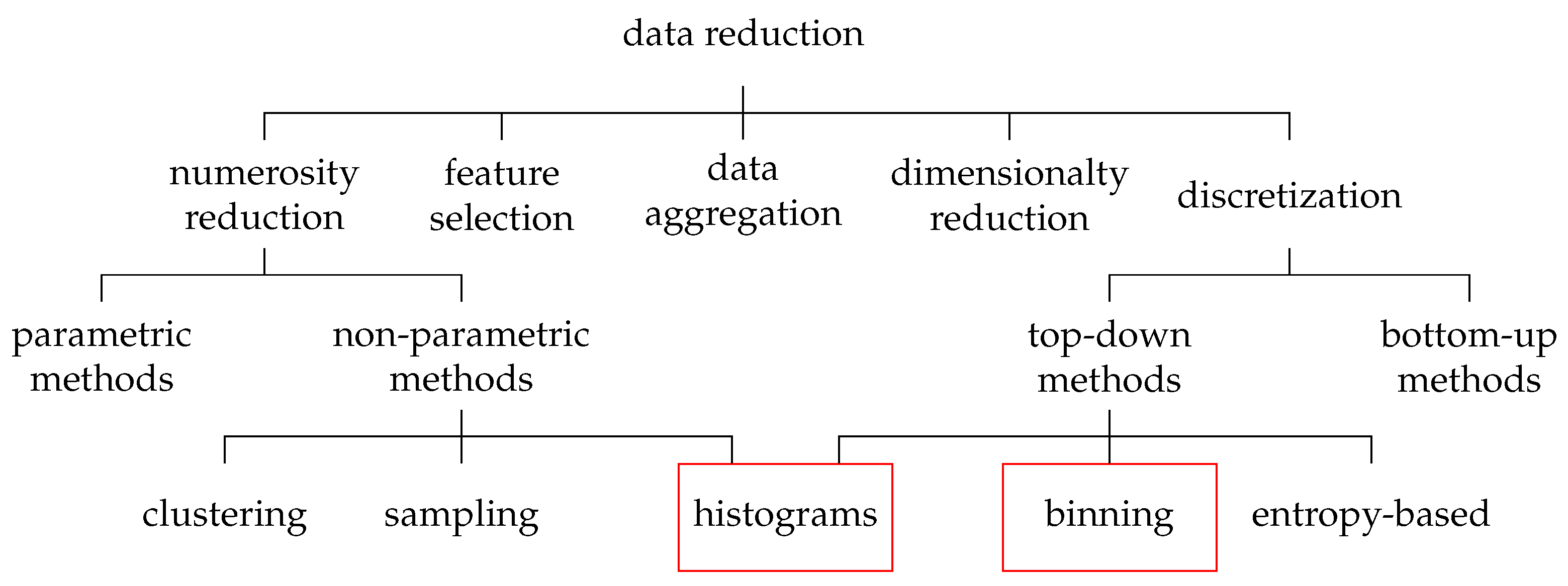
Several methods for data reduction already exist, most of which can be roughly divided into five approaches (Figure 1) [19]: data aggregation, feature selection, numerosity reduction, dimensionality reduction, and discretization. All these methods aim to obtain a reduced representation of the data set without reducing the information value.
Data aggregation describes the process of gathering data and presenting it in summarized form. This includes, for example, the summation of monthly data when only annual data are required, as well as the merging of multiple data sources.
Feature selection aims to identify and remove irrelevant, weakly relevant, or redundant features from the data set.
Numerosity reduction aims to reduce the number of samples in the data set (e.g., by deleting samples). Likewise, data can be replaced with alternative smaller representations or estimated.
Dimensionality reduction aims at reducing the amount of dimensions/features. Hereby, it is attempted to filter out features with a low informational value for the model or to aggregate several features. The most popular method of dimensionality reduction is the principal component analysis (PCA).
Data discretization refers to methods of reducing the number of data values by converting continuous data into a finite set of intervals. In order to simplify the original data, labels can then be used to replace the actual values.
In this paper, an approach called multidimensional binned reduction (MdBR) is presented. With respect to the presented data reduction taxonomy (Figure 1), it merges top-down discretization approaches with a non-parametric numerosity reduction via histograms. MdBR has linear complexity and can be facilitated to reduce large multivariate data sets to smaller subsets, which could be used for model training. The approach works best for large data sets of low-dimensional and periodic data. In addition to less data storage space and a faster training time, the approach also renders the need for extra under/over-sampling strategies of imbalanced data sets superfluous. The approach is based on discretizing the data using the bins of a multidimensional histogram. Afterwards, numerosity reduction is achieved by reducing the number of samples in each bin.
The MdBR approach is validated by reducing an extensive PV generation data set of about 92 million samples. The reduced data set is subsequently used to train a multilayer perceptron (MLP) model to estimate the output power of the system.
The results show that using the approach, the number of samples for training could be reduced by more than , while also increasing the model’s performance. Using the MdBR training sets, the training time was reduced from several hours to just a few minutes, rendering the approach valuable for applications where multiple models have to be trained, such as hyperparameter searches [21].
The remainder of the paper is structured as follows: In Section 2 an overview of the related work is presented. Section 3 introduces the proposed MdBR approach in detail, followed by a proof of concept in Section 4 demonstrating its efficiency on a use case. In the concluding Section 5, the results are summed up; including a future outlook of the paper.
2. Related Work
In order to extract a smaller training set from a larger data set, the most straightforward approach is to use probabilistic methods, which initially came from statistics.
One easy way is using sampling techniques such as Simple Random Sampling, where a fixed amount of samples is randomly picked from the larger set. Other approaches such as Separate Sampling [22], Balanced Sampling [23] or Stratified Ordered Selection [20] can also be applied but need the data to be structured in the form of classes, clusters or labels. However, most real measurement sets are not structured.
Another difficulty of real data sets is that they often have a strong class imbalance, which can lead to over-fitting when training the model [13,15]. A possible approach to counteract over-fitting is to remove the imbalance by over-sampling the minority samples. A common approach is the Synthetic Minority Over-sampling Technique (SMOTE) [24]. Furthermore, it is possible to solve the imbalance by under-sampling the majority samples. For this purpose, it is convenient to delete the duplicate or uninformative sample and thus reduce the redundancy [14,15]. However, which sample can be deemed as redundant is usually not easy to determine, especially if the data are not segmented into classes or discrete values.
Another approach to reduce the training data is the use of coresets. Coresets are weighted subsets of the full data set, which guarantee that solutions found on the coreset are competitive with solutions found on the full data set [25]. They can be constructed in various ways, but often, they rely too greatly on the aforementioned sampling approaches. Because coresets are guaranteed to represent the statistical properties of the full data set, their formation can be arbitrarily complex. Coresets are mostly used for classification tasks.
Instead of using a subset of the original data set, it is also possible to use a much smaller synthetic set facilitating a procedure called data set distillation [26]. With data set distillation it is possible to construct very small synthetic data sets, albeit to the disadvantage of a large computational overhang and poor generalization properties of the data set.
To reduce the number of samples, ref. [27] proposed a method called Principal Sample Analysis (PSA). In PSA, all samples in the set are ranked with regard to how well they could be used to discriminate between classes in the data. In each iteration of the algorithm, the lowest-ranked samples are removed. Another sample ranking scheme is presented in [11]. Here, several models are trained using different subsets in order to extract the samples proving to be most useful for the model. However, both methods do not scale well with large data sets, need already labeled data and are designed for classification tasks.
To find clusters in data sets, many other approaches are based on the k-nearestneighbor (kNN) [28] or k-means method [15,29]. Both approaches are used to assign similar samples to a cluster. Samples in the same cluster could then be combined to reduce the data set. However, kNN and k-means have a complexity that increases super-linearly with the number of samples and are thus only usable with great effort for large data sets [28].
Another possibility to cluster samples are top-down methods such as discretizing data via histograms. In contrast to bottom-up methods such as kNN, these clusters are not representative. However, at the same time, top-down methods are often significantly faster. Ref. [30] used educational data that were discretized by a histogram to train an ensemble of models for classification. Ref. [29] compared several discretization techniques (among others interval binning and k-means clustering) to discretize continuous clinical data. Afterward, classification models were trained with each approach, yielding that interval binning provided the worst model, whereas k-means proved to be more accurate. An evaluation of discretization techniques has also been performed by [31,32], concluding that the use of discretized data often yields an increased model accuracy after training, compared to undiscretized data. However, in both publications, the models are limited to classification tasks and data sets including a maximum of 2200 samples.
3. Methodology
In the following, the developed method of multidimensional binned reduction (MdBR) is presented. The method aims at particularly large, multivariate data sets with continuous and periodic data. However, it is also applicable for discrete or classified data. The method’s goal is to reduce the number of samples significantly in the data set for training models, without degrading the quality of the model.
3.1. Multidimensional Bin Reduction
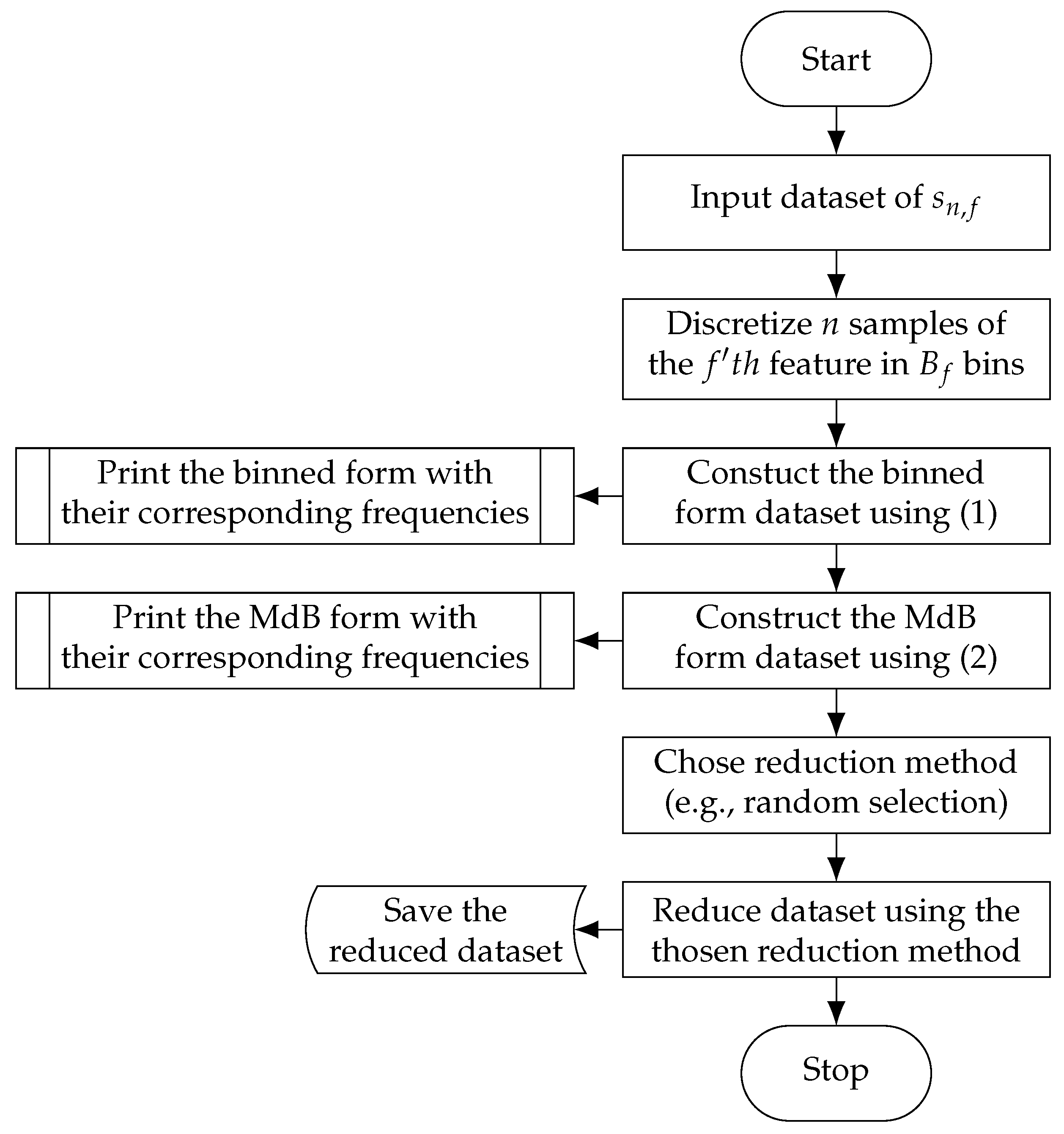
The initial setup is an extensive data set consisting of F features and N samples. Each continuous feature f of the data set was first discretized individually. Similar to a histogram, for each feature, the number of bins B was determined, and then it was calculated in which bin b the respective value s of the sample n and feature f was located. In this way, each sample was converted from its raw form into a binned form (see Equation (1)). For already discrete features, no binning was necessary:
Afterward, the bins of each sample are aggregated to a multidimensional bin (MdB), which could be understood as a value-dependent sample identifier (ID):
As each sample MdB is value-dependent, samples with identical bins were assigned to the same MdB. Assuming that each feature has been divided into a sufficiently large number of bins , the number of samples in each MdB corresponds to the number of samples, which can be assumed to be equal and hence redundant.
Although, theoretically, many different discretization techniques could be used for intervalizing the data, many are not suitable for large data sets. Due to the size of the training set and the computational effort involved, a top-down method such as a histogram is most appropriate.
The N samples of the first feature are divided into bins, bins for the second feature and, similarly, bins for the last feature. For making the MdB, we need the combination of the bins for each feature. So, the maximum number of different MdBs is equal to . However, the MdBs in the data set are only uniformly occupied if all samples in the data set are uniformly distributed, which is not the case for most real-world data sets. Especially in the case of periodic data, it is therefore unlikely that the number of MdBs represented in the data set will even come close to the maximum number of possible MdBs. Dependent on the size of the data set, is it also likely that the maximum number of possible MdBs is several orders of magnitude higher than the number of samples in the data set.
Since all samples assigned to the same MdB are redundant to each other, these samples do not add any value in terms of new information in the training set and can therefore be removed. Thus, only one sample per MdB is used for the training set.
Instead of removing redundant samples, it is also conceivable to calculate a representative sample for each MdB, e.g., by a clustering procedure or simple calculation of the mean value. Again, the number of samples in the training set is equal to the number of MdBs found.
A full example of the process can be seen in Figure 2.
3.2. Data Set Test
By using top down discretization methods such as histograms, MdBR has a linear complexity, which makes the method particularly suitable for large data sets. Furthermore, the method works best with low-dimensional data sets that exhibit periodic behavior. The periodic behavior leads to the fact that individual system states are reached recurrently. Exactly such states often lead to redundant information, which can be reduced with MdBR.
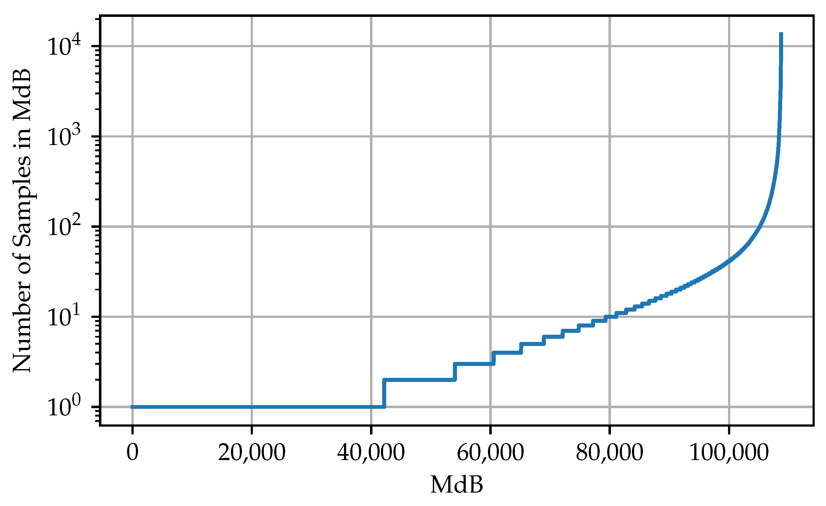
To test if a data set is usable, it is often sufficient to look at a small part of the set. However, the part should extend over several periods. For the test, first the MdBs of the samples of the selected section are calculated as explained in Section 3.1. Afterwards, the commonness of the individual MdBs in the section is evaluated. In the optimal case, the plotted commonness shows an exponential behavior (see Figure 3). This indicates that the majority of the samples is concentrated on a few MdBs. Theoretically, MdBR can be applied as soon as two or more samples are assigned to the same MdB. The more samples belonging to the same MdB, the more effective the reduction.
4. Numerical Study
In the following chapter, a proof of concept of the MdBR is presented. For this purpose, an multilayer perceptron (MLP) model was trained to estimate the AC output power of a PV system.
All tests were run on a virtual machine using 16 GB RAM and 2 vCPUs of an Intel Xeon Gold 6246 processor.
4.1. Data Set
A subset of the NIST Campus Photovoltaic data set was used as the basis to train the model. The whole data set is open source and publicly available at [33].
The data set includes real measured values from several PV systems located in Gaithersburg, Maryland, USA. For the proof of concept, the subset of the roof tilted array system in the period from 1 January 2015 to 31 December 2017 with a second-by-second resolution was selected. The considered system consists of 312 PV modules with a rated DC output power of 73.3 kW, feeding a single indoor inverter. Since the data set contains various channels that are not relevant for estimating the AC output power of the inverter, only a selection of channels were used (see Table 1).
To work with the data, as a first step, the set was cleaned by removing samples with missing or malicious values. In addition, since most neural networks show superior performance using normalized data, all features were scaled to a range between zero and one. All preprocessing resulted in a data set containing 6 features with 92,787,245 samples.
4.2. Feasibility Test
After cleaning the set, a test was performed to see if the data set was usable for MdBR at all (see Section 3.2). For this purpose, a small section of the data set was selected, and the MdBs were calculated. May 2017 and a number of 50 bins per feature were arbitrarily chosen. The goal was to see how the samples are distributed across the MdBs. The results of the feasibility test can be seen in Table 2.
When sorting the MdBs of the test by prevalence (see Figure 3), it can be seen that the vast majority of samples are located in only a small amount of MdB, reaching up to 13,545 samples in a single MdB. Therefore, considering the distribution of the sample in the data set, MdBR seems to be a good approach for reduction.
4.3. Neural Network
To ensure good comparability, the same neural network topology is used throughout the whole experiment.
The network consists of an input layer of 5 neurons (1 for each input feature) followed by 2 dense hidden layers of 20 neurons with a dropout rate of 10%. Finally, the hidden layers are followed by an output layer consisting of a single neuron. To allow the network to map nonlinear behavior, the second hidden layer and the output layer are provided with a activation function. An optimizer with a batch size of 20 was chosen for training.
Each time the network is generated, it is initialized with a random set of weights. This could cause the network to converge differently during training. In order to account for this random factor, each training set is used to train 20 models to calculate an averaged prediction error.
4.4. Training Set Generation Using MdBR
To generate the training and test set, the preprocessed data set was first shuffled and then split using 90% of the data for training and 10% of the data for testing/validation. Resulting in a training set of 83,508,520 samples and a test set of 9,278,725 samples.
To test the efficiency of the MdBR, the training set was then processed further to generate several reduced training sets. As mentioned before (see Section 3), a top-down method such as a histogram is most appropriate for the discretization process, due to the size of the training set and the computational effort involved. In [34], fixed bin width histograms were compared to adaptive histograms whose bin width is derived from a fixed number of samples per bin. It was found that fixed-bin-width histograms for a large number of samples seem to have better performance. Therefore, for each reduced data set, the training data were discretized using a different number of fixed-width bins.
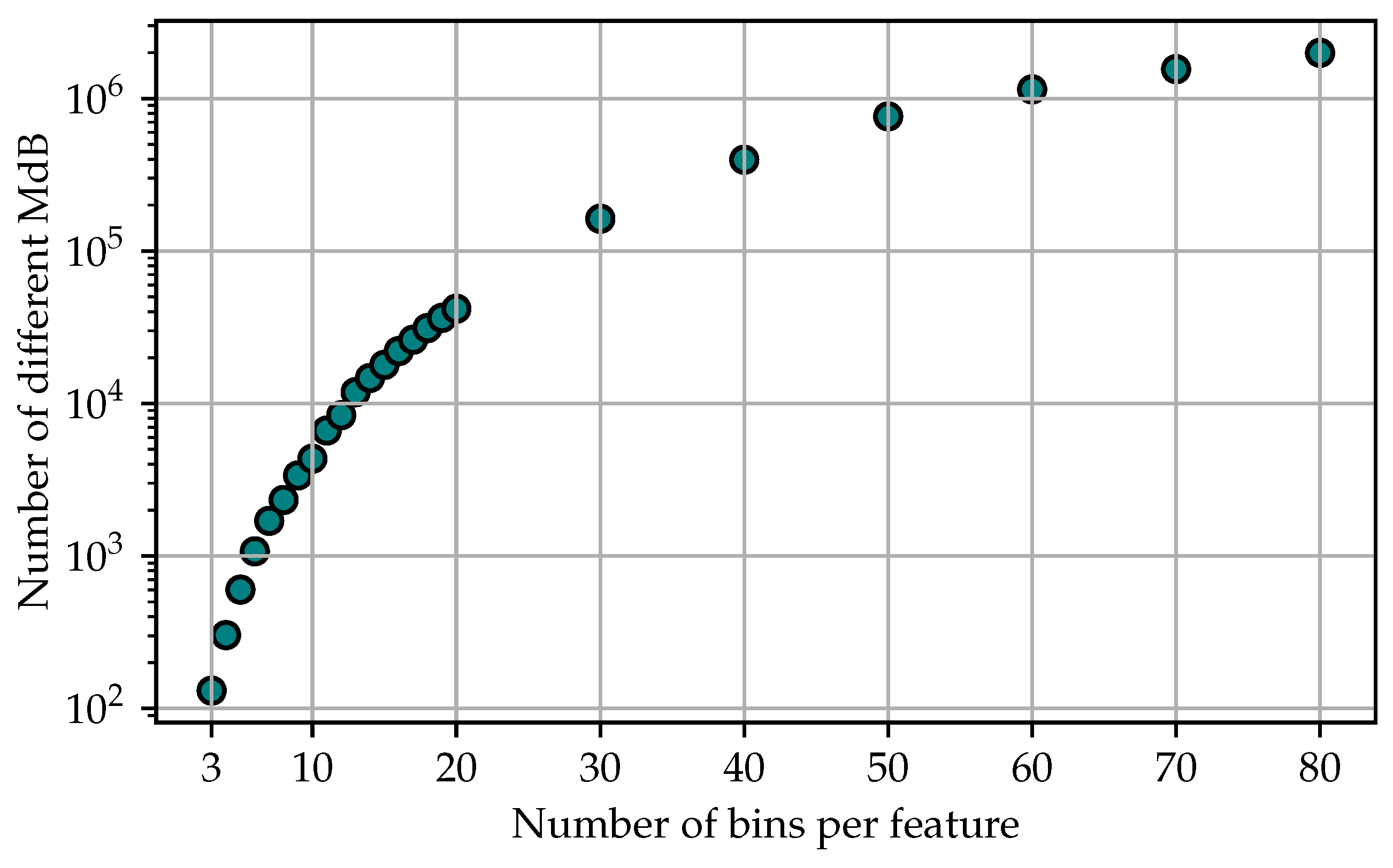
After the data for each training set are discretized, it comes to the reduction step. To reduce the training sets, two methods of MdBR were tested: reduction by random selection and reduction by representation using the mean. In the reduction by random selection sets, for each MdB, one of the samples assigned to the respective MdB is selected randomly. The rest of the samples are discarded. In the following, these data sets will be referred to as Random Selection In the reduction by representation sets, for each MdB, a representative sample is calculated using the mean value of all samples belonging to the respective MdB. Again, the reduced sets are thus formed by just one sample per MdB. In the following, these data sets will be referred to as Representative. The used number of bins and the size of the resulting training sets can be seen in Figure 4.
In total, 50 subsets were generated. One large unreduced baseline training set, one unreduced testing set, 24 reduced sets using the Random Selection method and 24 reduced sets using the Representative method.
Figure 5 shows the distribution of the normalized output power in some of the reduced training data sets. It can be seen that the distribution varies strongly depending on the number of bins, resulting in the training not providing the same sample distribution as the original data set if a small number of bins is used.
4.5. Training Results
The full/unreduced data set was first used to train models to obtain a baseline for comparability. As a performance metric the root-mean-square error (RMSE) was used, which (as the output is normalized between zero and one) can be rendered as the deviation in percent using the normalized root-mean-square error (NRMSE).
The average result of the baseline models can be seen in Table 3.
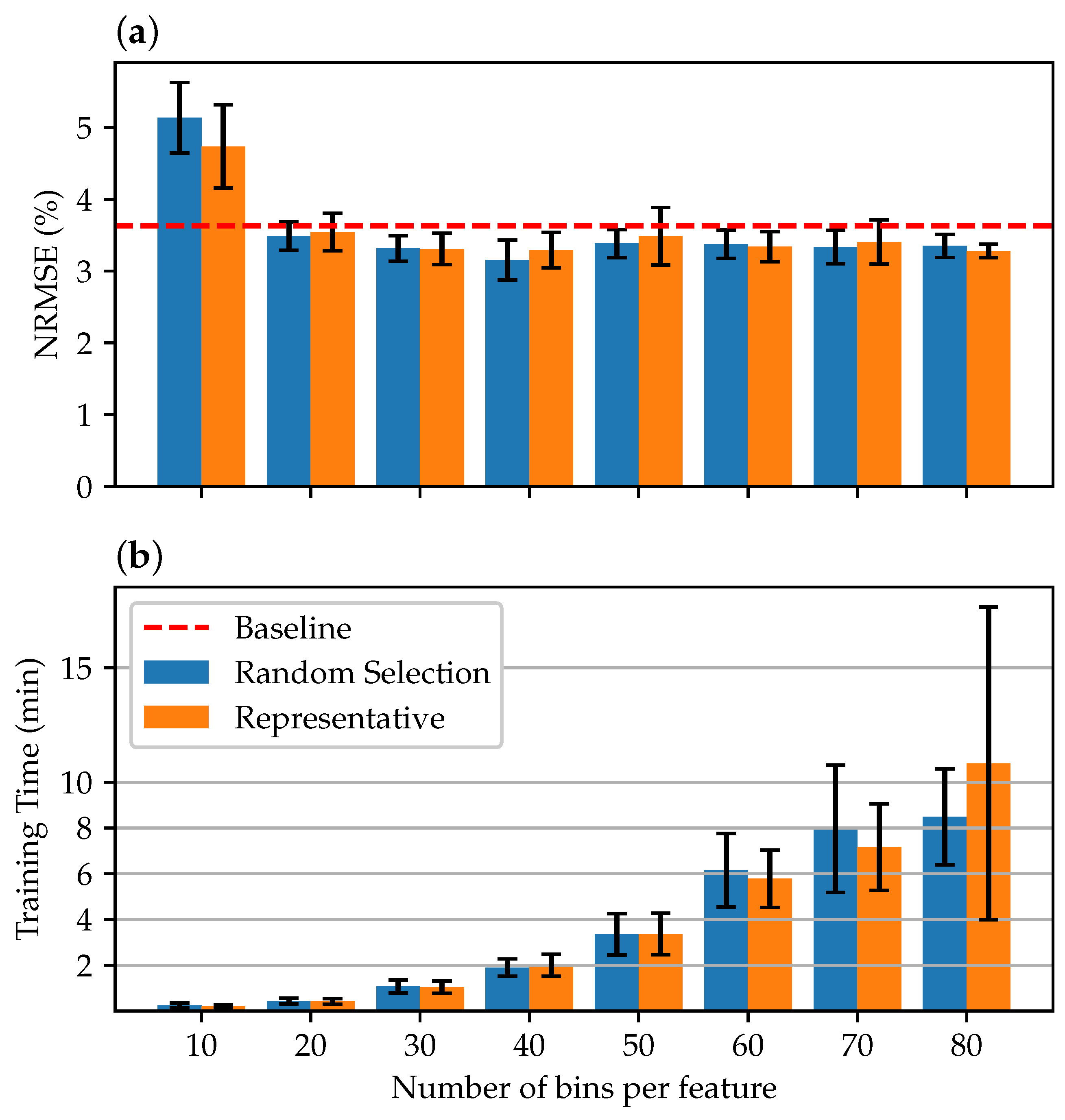
In the further course, tests were carried out using the reduced training data sets. First, an extensive range of bins was considered. Figure 6 shows the results from 10 to 80 bins per feature. It can be seen that already, with a relatively small number of 20 bins per feature, the average accuracy of the models is at least comparable to the accuracy of the baseline models. At a number of 40 bins, the maximum accuracy is reached. If the number of bins is increased further, it is not reflected in a further increase in accuracy. However, the time required for training increases as the data are segmented into more MdB, increasing the training set size.
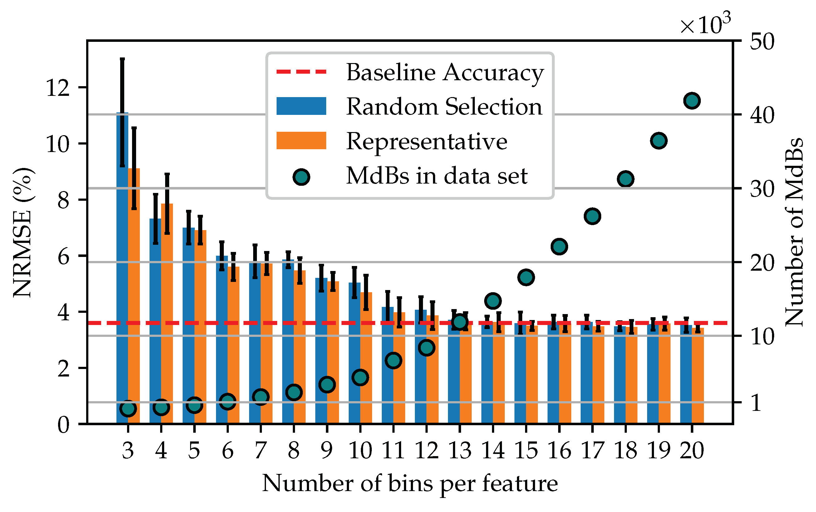
A more detailed view of the model accuracy for the reduced data sets of 3–20 bins is shown in Figure 7. Along with a plot of the number of MdBs that make up each training set. It can be seen that for a data set reduced by MdBR using 13 bins per feature, the accuracy of the model is equal to the baseline accuracy. In addition, the performance of data sets formed by the representative procedure seems to be slightly better than that of the random selection procedure.
4.6. Discussion
The proof of concept demonstrated that, in addition to a significant reduction in the training set, the model’s accuracy could also be constantly improved. Thus, a model comparable to the baseline could be trained with only 13 bins per feature. This corresponds to the use of 11,869 samples, which is of the entire training data set. The best models could be trained using about 40 bins, corresponding to of the data set.
Starting from a size of 20 bins, models could be trained consistently better than the baseline model. This effect was also observed by [31,32] using discretized data (without reduction) for classification tasks and by [11] (image classification) and [35] (language processing) after removing redundant or duplicate samples from the training sets. Most likely, it can be explained with the model having better generalization capabilities after being trained with a reduced or non-redundant data set.
When looking at Figure 6, it is also noticeable that the error increases again with a further increase in the bins if more then 40 bins are used. This could be caused by the model losing its superior generalization ability when confronted with larger training sets. Whether this behavior is systematic would have to be investigated using several data sets. However, since the variances in the trained models are overlapping, it is also conceivable that this is a statistical fluctuation due to the randomized initialization of the models. Therefore, it could be possible that the better model with 40 bins is rather to be interpreted as an outlier in the context of the natural model variance instead of being a constant minimum. In general, it must be assumed that the optimal number of bins depends on the particular data set as well as the individual feature.
Furthermore, since for comparability reasons, all models were trained using the same hyperparameter (e.g., network size, optimizer, batch size). It has to be assumed that there is room for further improvement of the models.
Considering the two tested reduction methods, there seemed to be no significant difference between a training set of randomly selected samples of each MdB or representative samples using the mean of each MdB.
5. Conclusions
In this paper, the numerosity reduction procedure MdBR was presented. The procedure rests upon the discretization of continuous data and the subsequent removal of redundant samples.
The proof of concept showed that the size of the training data set could be reduced by , leading to smaller storage space and faster training time. In addition, higher prediction accuracy was achieved. The reduced training time renders MdBR suitable for processes where many models have to be trained, e.g., hyperparameter search for neural networks.
As a positive side effect, the MdBR approach also limits the thread of over-fitting due to an imbalanced training set and lessens the influence of measurement noise.
MdBR works best with large data sets of low-dimensional data. Although periodic data often include the most redundant samples and thus provide the best reduction capabilities, the presented MdBR approach can only handle individual samples (time-invariant data) and not sequences of samples, as often done in time series. Nevertheless, it could be applied to sequences by transforming the sequence into a single vector. One possibility would be by flattening the lagging/leading observations into the feature vector. On the downside, this would increase the dimensionality and thus lessen the effect of the reduction. Another possibility would be to encode the sequences into a latent space consisting of a single vector. Whether this is worthwhile or whether there are other possibilities for the reduction in data sets of sequences is the subject of future evaluations.
Also pending is an evaluation of the approach by further data sets and the question of how far different discretization techniques influence MdBR.
Author Contributions
Conceptualization, J.W., P.T.B., and S.R.; methodology, J.W.; software, J.W.; validation, J.W., P.T.B., and S.R.; investigation, J.W.; writing—original draft preparation, J.W.; writing—review and editing, J.W., P.T.B., and S.R.; visualization, J.W.; supervision, P.T.B.; project administration, S.R.; funding acquisition, S.R. All authors have read and agreed to the published version of the manuscript.
Funding
This research was funded by the German Bundesministerium für Bildung und Forschung (BMBF) grant number 13FH094PB8.
Institutional Review Board Statement
Not applicable.
Informed Consent Statement
Not applicable.
Data Availability Statement
The dataset used in this study is publicly available: [33].
Conflicts of Interest
The authors declare no conflict of interest. The funders had no role in the design of the study; in the collection, analyses, or interpretation of data; in the writing of the manuscript, or in the decision to publish the results.
References
- Malik, H.; Fatema, N.; Iqbal, A. Intelligent Data-Analytics for Condition Monitoring: Smart Grid Applications; Academic Press: Cambridge, MA, USA, 2021. [Google Scholar]
- Teimourzadeh Baboli, P.; Babazadeh, D.; Raeiszadeh, A.; Horodyvskyy, S.; Koprek, I. Optimal temperature-based condition monitoring system for wind turbines. Infrastructures 2021, 6, 50. [Google Scholar] [CrossRef]
- Alzawaideh, B.; Baboli, P.T.; Babazadeh, D.; Horodyvskyy, S.; Koprek, I.; Lehnhoff, S. Wind Turbine Failure Prediction Model using SCADA-based Condition Monitoring System. In Proceedings of the 2021 IEEE Madrid PowerTech, Madrid, Spain, 28 June–2 July 2021; pp. 1–6. [Google Scholar]
- Berghout, T.; Benbouzid, M.; Bentrcia, T.; Ma, X.; Djurović, S.; Mouss, L.H. Machine Learning-Based Condition Monitoring for PV Systems: State of the Art and Future Prospects. Energies 2021, 14, 6316. [Google Scholar] [CrossRef]
- Wani, S.A.; Rana, A.S.; Sohail, S.; Rahman, O.; Parveen, S.; Khan, S.A. Advances in DGA based condition monitoring of transformers: A review. Renew. Sustain. Energy Rev. 2021, 149, 111347. [Google Scholar] [CrossRef]
- Lee, S.B.; Stone, G.C.; Antonino-Daviu, J.; Gyftakis, K.N.; Strangas, E.G.; Maussion, P.; Platero, C.A. Condition monitoring of industrial electric machines: State of the art and future challenges. IEEE Ind. Electron. Mag. 2020, 14, 158–167. [Google Scholar] [CrossRef]
- Zainuddin, N.M.; Rahman, M.A.; Kadir, M.A.; Ali, N.N.; Ali, Z.; Osman, M.; Mansor, M.; Ariffin, A.M.; Rahman, M.S.A.; Nor, S.; et al. Review of Thermal Stress and Condition Monitoring Technologies for Overhead Transmission Lines: Issues and Challenges. IEEE Access 2020, 8, 120053–120081. [Google Scholar] [CrossRef]
- Yüce, F.; Hiller, M. Condition Monitoring of Power Electronic Systems through Data Analysis of Measurement Signals and Control Output Variables. IEEE J. Emerg. Sel. Top. Power Electron. 2021. [Google Scholar] [CrossRef]
- Gonzalez-Abreu, A.D.; Saucedo-Dorantes, J.J.; Osornio-Rios, R.A.; Arellano-Espitia, F.; Delgado-Prieto, M. Deep Learning based Condition Monitoring approach applied to Power Quality. In Proceedings of the 2020 25th IEEE International Conference on Emerging Technologies and Factory Automation (ETFA), Vienna, Austria, 8–11 September 2020; Volume 1, pp. 1427–1430. [Google Scholar]
- Hestness, J.; Narang, S.; Ardalani, N.; Diamos, G.; Jun, H.; Kianinejad, H.; Patwary, M.; Ali, M.; Yang, Y.; Zhou, Y. Deep learning scaling is predictable, empirically. arXiv 2017, arXiv:1712.00409. [Google Scholar]
- Lapedriza, A.; Pirsiavash, H.; Bylinskii, Z.; Torralba, A. Are all training examples equally valuable? arXiv 2013, arXiv:1311.6510. [Google Scholar]
- Dhar, S.; Guo, J.; Liu, J.; Tripathi, S.; Kurup, U.; Shah, M. On-device machine learning: An algorithms and learning theory perspective. arXiv 2019, arXiv:1911.00623. [Google Scholar] [CrossRef]
- Barandela, R.; Valdovinos, R.M.; Sánchez, J.S.; Ferri, F.J. The imbalanced training sample problem: Under or over sampling? In Joint IAPR International Workshops on Statistical Techniques in Pattern Recognition (SPR) and Structural and Syntactic Pattern Recognition (SSPR); Springer: Berlin/Heidelberg, Germany, 2004; pp. 806–814. [Google Scholar]
- Gong, Z.; Zhong, P.; Hu, W. Diversity in machine learning. IEEE Access 2019, 7, 64323–64350. [Google Scholar] [CrossRef]
- Karystinos, G.N.; Pados, D.A. On overfitting, generalization, and randomly expanded training sets. IEEE Trans. Neural Netw. 2000, 11, 1050–1057. [Google Scholar] [CrossRef] [PubMed]
- Bottou, L.; Lin, C.J. Support vector machine solvers. Large Scale Kernel Mach. 2007, 3, 301–320. [Google Scholar]
- Balduin, S.; Oest, F.; Blank-Babazadeh, M.; Nieße, A.; Lehnhoff, S. Tool-assisted surrogate selection for simulation models in energy systems. In Proceedings of the 2019 Federated Conference on Computer Science and Information Systems (FedCSIS), Leipzig, Germany, 1–4 September 2019; pp. 185–192. [Google Scholar]
- Hospedales, T.; Antoniou, A.; Micaelli, P.; Storkey, A. Meta-learning in neural networks: A survey. arXiv 2020, arXiv:2004.05439. [Google Scholar] [CrossRef] [PubMed]
- Han, J.; Pei, J.; Kamber, M. Data Mining: Concepts and Techniques; Elsevier: Amsterdam, The Netherlands, 2011. [Google Scholar]
- Kalegele, K.; Takahashi, H.; Sveholm, J.; Sasai, K.; Kitagata, G.; Kinoshita, T. Numerosity reduction for resource constrained learning. J. Inf. Process. 2013, 21, 329–341. [Google Scholar] [CrossRef] [Green Version]
- Feurer, M.; Hutter, F. Hyperparameter optimization. In Automated Machine Learning; Springer: Cham, Switzerland, 2019; pp. 3–33. [Google Scholar]
- Shahrokh Esfahani, M.; Dougherty, E.R. Effect of separate sampling on classification accuracy. Bioinformatics 2014, 30, 242–250. [Google Scholar] [CrossRef]
- Deville, J.C.; Tillé, Y. Efficient balanced sampling: The cube method. Biometrika 2004, 91, 893–912. [Google Scholar] [CrossRef] [Green Version]
- Chawla, N.V.; Bowyer, K.W.; Hall, L.O.; Kegelmeyer, W.P. SMOTE: Synthetic minority over-sampling technique. J. Artif. Intell. Res. 2002, 16, 321–357. [Google Scholar] [CrossRef]
- Bachem, O.; Lucic, M.; Krause, A. Practical coreset constructions for machine learning. arXiv 2017, arXiv:1703.06476. [Google Scholar]
- Wang, T.; Zhu, J.Y.; Torralba, A.; Efros, A.A. Dataset distillation. arXiv 2018, arXiv:1811.10959. [Google Scholar]
- Ghojogh, B.; Crowley, M. Principal sample analysis for data reduction. In Proceedings of the 2018 IEEE International Conference on Big Knowledge (ICBK), Singapore, 17–18 November 2018; pp. 350–357. [Google Scholar]
- Mall, R.; Jumutc, V.; Langone, R.; Suykens, J.A. Representative subsets for big data learning using k-NN graphs. In Proceedings of the 2014 IEEE International Conference on Big Data (Big Data), Washington, DC, USA, 27–30 October 2014; pp. 37–42. [Google Scholar]
- Maslove, D.M.; Podchiyska, T.; Lowe, H.J. Discretization of continuous features in clinical datasets. J. Am. Med. Inform. Assoc. 2013, 20, 544–553. [Google Scholar] [CrossRef] [Green Version]
- Dimić, G.; Rančić, D.; Pronić-Rančić, O.; Milošević, D. An approach to educational data mining model accuracy improvement using histogram discretization and combining classifiers into an ensemble. In Smart Education and e-Learning 2019; Springer: Berlin/Heidelberg, Germany, 2019; pp. 267–280. [Google Scholar]
- Hacibeyoglu, M.; Arslan, A.; Kahramanli, S. Improving classification accuracy with discretization on data sets including continuous valued features. Ionosphere 2011, 34, 2. [Google Scholar]
- Dougherty, J.; Kohavi, R.; Sahami, M. Supervised and unsupervised discretization of continuous features. In Machine Learning Proceedings 1995; Elsevier: Amsterdam, The Netherlands, 1995; pp. 194–202. [Google Scholar]
- Boyd, M.; Chen, T.; Doughert, B. NIST Campus Photovoltaic (PV) Arrays and Weather Station Data Sets; National Institute of Standards and Technology [Data Set]; U.S. Department of Commerce: Washington, DC, USA, 2017. [CrossRef]
- Scott, D.W. Multivariate Density Estimation: Theory, Practice, and Visualization; John Wiley & Sons: Hoboken, NJ, USA, 2015. [Google Scholar]
- Lee, K.; Ippolito, D.; Nystrom, A.; Zhang, C.; Eck, D.; Callison-Burch, C.; Carlini, N. Deduplicating training data makes language models better. arXiv 2021, arXiv:2107.06499. [Google Scholar]
Figure 1.
Taxonomy of data reduction approaches (based on [19,20]). Marked in red are the approaches from which principles are integrated into the presented multidimensional binned reduction (MdBR) procedure.

Figure 2.
Process flowchart of the multidimensional binned reduction (MdBR).

Figure 3.
Plotted results of the feasibility test using the data of May 2017. The MdBs are sorted by prevalence.
Figure 3.
Plotted results of the feasibility test using the data of May 2017. The MdBs are sorted by prevalence.

Figure 4.
Size of the reduced training sets with a different number of bins per feature. The number of different MdBs per data set is equal to the number of samples in the training set.
Figure 4.
Size of the reduced training sets with a different number of bins per feature. The number of different MdBs per data set is equal to the number of samples in the training set.

Figure 5.
Distribution of the normalized output power in the training set after reducing with the respective number of bins per feature.
Figure 5.
Distribution of the normalized output power in the training set after reducing with the respective number of bins per feature.

Figure 6.
Comparison of the model average accuracy (a) and training time (b) using 10 to 80 bins per feature for reducing the training data set. Each model has been trained 20 times.
Figure 6.
Comparison of the model average accuracy (a) and training time (b) using 10 to 80 bins per feature for reducing the training data set. Each model has been trained 20 times.

Figure 7.
Comparison of the model average accuracy using 3 to 20 bins per feature for reducing the training data set. The number of different MdBs per data set is equal to the samples. Each model has been trained 20 times.
Figure 7.
Comparison of the model average accuracy using 3 to 20 bins per feature for reducing the training data set. The number of different MdBs per data set is equal to the samples. Each model has been trained 20 times.


Table 1.
Used Channels from the Roof tilted Array PV System subset.
| Features/Channels | Abbreviation |
|---|---|
| AC real power | PwrMtrP_kW |
| Outdoor ambient temperature | SEWSAmbientTemp_C |
| Module Temperature | SEWSModuleTemp_C |
| Plane of array irradiance | SEWSPOAIrrad_Wm2 |
| Inverter heatsink temperature | InvTempHeatsink_C |
| Inverter operating status | InvOpState |
Table 2.
Properties and results of the feasibility test.
| Artifact | Value |
|---|---|
| Period | May 2017 |
| Number of samples | 2,671,113 |
| Number of bins per feature | 50 |
| Number of possible MdB | |
| Number of found MdB | 108,733 |
| Max. sample in one MdB | 13,545 |
Table 3.
Results of the generated baseline, averaged over 20 models.
| Artifact | Value |
|---|---|
| Number of training samples | 83,508,520 |
| NRMSE | |
| Training Time | 4 h:24 m ± 1 h:42 m |
Publisher’s Note: MDPI stays neutral with regard to jurisdictional claims in published maps and institutional affiliations. |
© 2022 by the authors. Licensee MDPI, Basel, Switzerland. This article is an open access article distributed under the terms and conditions of the Creative Commons Attribution (CC BY) license (https://creativecommons.org/licenses/by/4.0/).
Share and Cite
MDPI and ACS Style
Wibbeke, J.; Teimourzadeh Baboli, P.; Rohjans, S. Optimal Data Reduction of Training Data in Machine Learning-Based Modelling: A Multidimensional Bin Packing Approach. Energies 2022, 15, 3092. https://doi.org/10.3390/en15093092
AMA Style
Wibbeke J, Teimourzadeh Baboli P, Rohjans S. Optimal Data Reduction of Training Data in Machine Learning-Based Modelling: A Multidimensional Bin Packing Approach. Energies. 2022; 15(9):3092. https://doi.org/10.3390/en15093092
Chicago/Turabian StyleWibbeke, Jelke, Payam Teimourzadeh Baboli, and Sebastian Rohjans. 2022. "Optimal Data Reduction of Training Data in Machine Learning-Based Modelling: A Multidimensional Bin Packing Approach" Energies 15, no. 9: 3092. https://doi.org/10.3390/en15093092
Note that from the first issue of 2016, this journal uses article numbers instead of page numbers. See further details here.