Abstract
In recent years, verification and validation processes of automated driving systems have been increasingly moved to virtual simulation, as this allows for rapid prototyping and the use of a multitude of testing scenarios compared to on-road testing. However, in order to support future approval procedures for automated driving functions with virtual simulations, the models used for this purpose must be sufficiently accurate to be able to test the driving functions implemented in the complete vehicle model. In recent years, the modelling of environment sensor technology has gained particular interest, since it can be used to validate the object detection and fusion algorithms in Model-in-the-Loop testing. In this paper, a practical process is developed to enable a systematic evaluation for perception–sensor models on a low-level data basis. The validation framework includes, first, the execution of test drive runs on a closed highway; secondly, the re-simulation of these test drives in a precise digital twin; and thirdly, the comparison of measured and simulated perception sensor output with statistical metrics. To demonstrate the practical feasibility, a commercial radar-sensor model (the ray-tracing based RSI radar model from IPG) was validated using a real radar sensor (ARS-308 radar sensor from Continental). The simulation was set up in the simulation environment IPG CarMaker® 8.1.1, and the evaluation was then performed using the software package Mathworks MATLAB®. Real and virtual sensor output data on a low-level data basis were used, which thus enables the benchmark. We developed metrics for the evaluation, and these were quantified using statistical analysis.
1. Introduction
In the field of driver assistance and active safety systems, an increasing level of automation has been introduced in public transport in recent years [1]. Automated vehicles will be able to detect and react to hazards and vulnerable road users faster and more appropriately than a human driver. This is expected to lead to a significant reduction in road accidents, as around 90 percent of accidents are primarily caused by human error, e.g., [2,3]. Taking the driver out of control will improve driving comfort by reducing the driver’s workload, especially in monotonous situations, such as traffic jams, where the driver is mentally under-challenged, or in cases where the driver is overloaded and cannot fully manage the traffic situation. The human driver can also perform other productive or enjoyable activities during the journey, thus, reducing the opportunity cost of time spent in the car.
Automated vehicles can significantly increase access and mobility for populations currently unable or not allowed to use conventional cars [4]. In addition, automated driving functions can improve fuel economy by providing more subtle acceleration and deceleration than a human driver. However, a number of issues remain to be resolved before self-driving vehicles become a reality.
Motivation
Increasing the level of driving automation leads to an increase in system complexity. Therefore, the number of test cases necessary to proof the functional safety increases exponentially [5]. The literature reports that hundreds of millions of accident-free driving kilometres are needed to prove that the system is better than human vehicle control in terms of vehicle safety, e.g., [6]. Therefore, testing and validation efforts are being shifted towards virtual validation as well as X-in-the-Loop methods [7]. An essential requirement for testing ADAS/AD systems in virtual space is the realistic modelling of the virtual environment required for the system under test.
Virtual testing is particularly suitable for testing safety-critical scenarios that are difficult, costly, unsafe and impossible to reproduce on test tracks or roads [8]. The development and testing of driving assistance and automated vehicle control systems is performed step by step, from simple object detection to highly sophisticated functions, in the phases defined in the V-Model presented in ISO 26262-2:2018 [9]. Accordingly, the virtual environment, as well as the architecture and capabilities of the sensor models used, will vary according to the development phases [10].
To accelerate the test execution, a possible, and in recent years, very relevant solution is provided by the use of simulation tools on a virtual basis [11,12]. In the case of perception–sensor models in early development phases, virtual simulation based on ideal or phenomenological sensor models has become established in the industry. These models can be used to test and validate the fundamental operating principles of control architectures.
Using advanced perception–sensor models enables the testing of machine-perception and sensor-fusion algorithms in a later stage, enabling thus a first parameter tuning on a complete vehicle level before the first prototype is built.
Since sensor models have a limited ability to represent reality, careful consideration must be given to whether the model is a satisfactory replacement for the real sensor for validating the safety of ADAS/AD functions. However, there is no accepted methodology available that objectively quantifies the quality of perception–sensor models. In the present paper, a novel approach to assess the performance of virtual perception model is described.
The rest of the paper is structured as follows: Section 2 reviews the state-of-the-art technology, Section 3 describes the used method including the digital twin of the driving environment, the vehicle and the assessment approach. Section 4 presents the results of the new performance evaluation method using the IPG RSI model compared to an automotive radar sensor already proven on the market. Section 5 discusses the results of the sensor performance assessment and describes the limitations detected during the research and gives an outlook on future improvements.
2. State-of-the-Art
The simulation of perception sensors has been a part of worldwide research in recent years. Vehicles equipped with Automated Driving or Advanced Driver Assistance functions perform their tasks based on information provided by sensors that sense the environment, such as different types of radar sensors, front-, rear-, surround-view and night-vision cameras, LIDAR sensors, ultrasonic sensors [13]. The reliability of the warning and intervention hardware components and the algorithms that control them is strongly influenced by the quality of the information provided by the perception sensors. One of the goals of virtual testing is to model the behaviour of these sensors to match their behaviour under real environmental conditions.
In the simplest case, it is sufficient for the sensor model to give a perfect representation of the environment, using information artificially generated from the scenario, such as the relative distance, relative velocity, angular position, classification etc., taking into account the sensor’s sensing properties, such as the maximum sensing range, horizontal and vertical coverage (FOV). This so called geometric or ideal sensor model is well suited to test the dynamic behaviour of complex systems at the whole vehicle level [14].
A more realistic modelling approach would be to implement physical sensor models simulating the behaviour of the complex interaction between sensors and the environment, such as the reflectivity, sight obstruction by other objects, multipath fluctuation, interference, damping etc.; however, the computational time and effort involved make the use of such models for vehicle testing impractical [15].
However, some sensor phenomena need to be modelled to test the performance of ADAS/AD systems with higher complexity. To test such systems under sub-optimal sensing conditions, sensor models are needed that reflect typical sensor phenomena based on the results of field tests, such as reduced range or increased noise levels in bad weather conditions, erroneous, missing or incomplete information on some sensed parameters, tracking errors, loss of objects etc. [16]. Models describing the phenomenological effects of different sensing technologies under similar conditions allow the performance and fault tolerance of the whole system chain to be investigated, taking into account an appropriate balance between the fidelity of the simulation, the complexity of the parameter settings and the computational power.
2.1. Classification of Virtual Sensor Models
Depending on the use case for virtual sensors, a general classification of sensor modelling approaches can be given. Using the basic simulation methodology, a model can be classified as a High-, Mid- or Low-Fidelity sensor model [10] or as black-, gray- or white-box [11]. As Peng in [17] and Schaermann in [18] denoted, there are three different modelling approaches for active perception sensors. These are the deterministic, the statistical and the field propagation approach; see Table 1. The deterministic modelling approach is based on mathematical formulations, which are represented by a multitude of parameters. If a sufficiently large amount of data is collected, the parameters can be trained and ideal sensor behaviour can be mapped.

Table 1.
Classification of sensor modelling methods according to [17,18].
The statistical approach is based on statistical distribution functions. This model is also called phenomenological sensor model and the realisations are drawn from a distribution function, which has to be determined before. This model architecture represents a good trade-off between computational effort and realism. This paper will focus on the validation of the third modelling approach, the field-propagation models. These models are simulating the propagation using Maxwell’s equations. As these equations only can be solved for few geometries, a numerical approximation must be used.
In the case of a radar sensor, the propagation of the wave can be approximated with the Finite-Difference Time-Domain (FDTD). In order to achieve a real-time capable simulation, FDTD is too expensive in terms of computational power. However, other methods to approximate Maxwell’s equations include the ray-optical approaches [17], simulating the propagation of electromagnetic waves by optical rays. Ray-tracing methods, like the published approach in [19], can model electromagnetic waves with various physical effects. For every radar transmitter–receiver pair, the wave propagation can be analysed to output the range and Doppler frequency for every detected target.
A major disadvantage of models based only on optics theory is that the effect of scattering is not included. Therefore, a scattering model must be implemented in the simulation. This can be either a stochastic scattering approach or a micro-facet-based scattering model as shown in [20]. By using these field-propagation models in the simulation environment, unprocessed environment sensor data with physical attributes are generated. This data is on a low-level in the signal processing chain, since it has not yet undergone any object detection or fusion algorithm.
2.2. Assessment Methods of Virtual Sensors
Virtual testing, for all its potential benefits, has limited fidelity because of its generalisation to the real environment. Sensor models represent reality only roughly or by focusing on a specific property of a sensor type. Therefore, it is necessary to assess whether a sensor model can sufficiently represent the real world to validate the safety of ADAS/AD systems. In the literature, several methods have been published on verification and validation methods for perception–sensor models [21,22,23]. All these approaches have their advantages and disadvantages and specific areas of application.
Depending on the general validation strategy and the accuracy of the available perceptual sensor models, different goals can be achieved with the virtual ADAS/AD validation. Therefore, it is difficult to quantify the performance of the different techniques since no accepted methodology to assess the performance of sensor models in the automotive spectrum exists today. One simple approach to assess the accuracy of a virtual sensor model can be to compare the performance of the ADAS/AD function within the virtual environment with its real world performance, running the same driving scenario [8]. This approach assumes that, for the assessment, models describing the ADAS/AD function under test are available in addition to sensor models of sufficient fidelity and that at least one prototype of the real hardware is available for real-world testing.
Since our hardware resources are limited to open-interface sensors freely available on the market, our sensor modelling efforts are designed accordingly. The present research introduces a novel approach that we call Dynamic Ground Truth—Sensor Model Validation (DGT-SMV) for performance assessment of perception–sensor models. The method is based on a statistical comparison of simulated and measured low-level radar data and aims to provide a quantifiable evaluation of the low-level radar-sensor model used. The method is presented in the next section.
3. Methodology
3.1. Dynamic Ground Truth Sensor Model Validation Approach
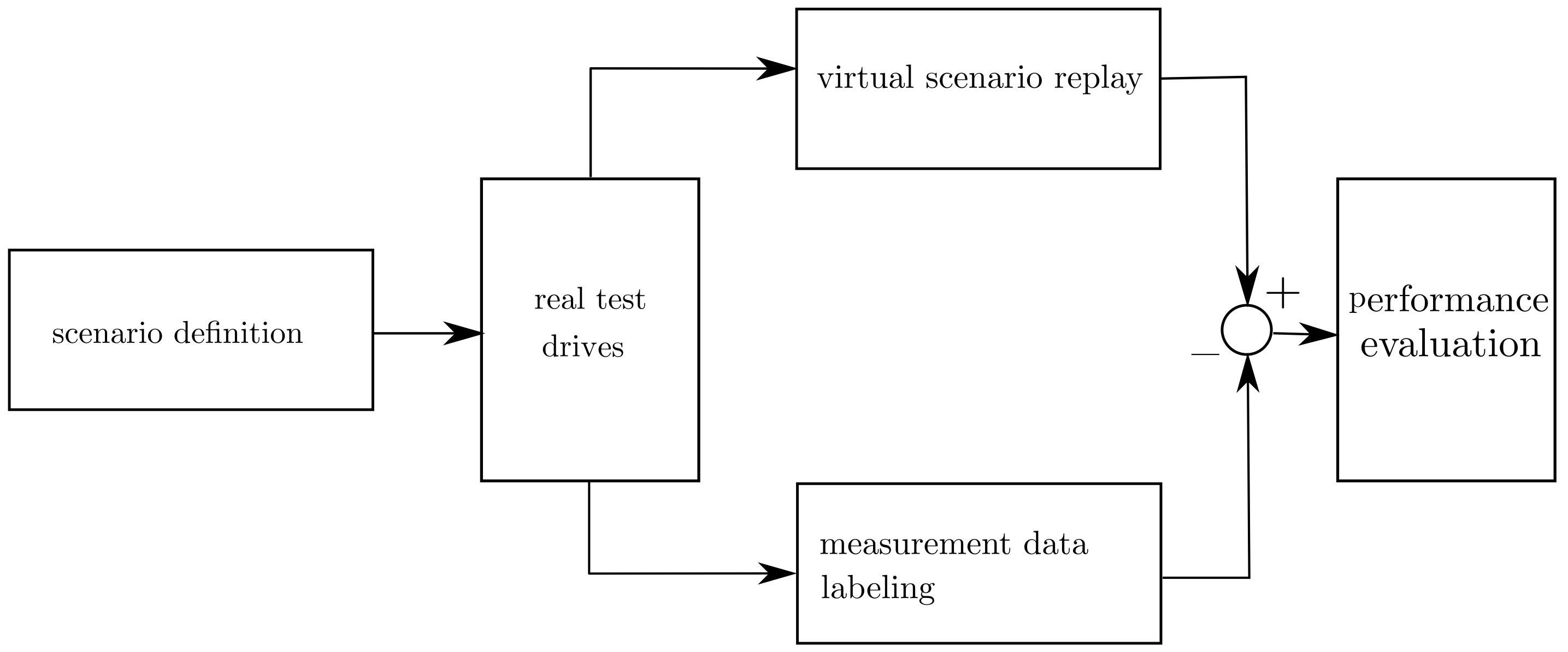
The DGT-SMV approach is depicted in Figure 1. The process starts with the definition of driving scenarios (scenario definition), which are related to phenomena of the evaluated sensor, such as multipath-propagation and separation capability [24,25]. In the next step, the tests are performed on a proving ground or in public traffic (real test drive), including an accurate measurement equipment.

Figure 1.
Dynamic ground truth sensor model validation process.
The measurement data is used to label the recorded low-level sensor output (measurement data labelling). For providing a method for direct comparison, the test drives are then re-simulated in a detailed virtual representation using a digital twin of the environment and the investigated virtual sensor (virtual sensor replay). The sensor then produces the virtual low-level sensor output that is finally compared with the measured sensor output (performance evaluation) with statistical methods. The individual steps in the DGT-SMV process are described in detail in the next sections.
3.2. On-Road Measurements
Virtual testing can be conducted on a road section edited with a simple road editor in the initial development phase; however, commercially available simulation programs can be also used to re-simulate the real-world measurements of road sections. Ultra-High-Definition Maps [25] allow the simulation of existing real road geometries, thus, facilitating the realistic modelling of the virtual environment. This method allows the analysis of the complete functional chain from detection of environment perception sensors to intervention systems.
On the digital map, one can accurately measure the position, direction and movement of the test vehicle, as well as the reference distance to static objects, such as lane markings, guardrails and curbs using a high precision inertial measurement unit (IMU). As part of the measurement campaign in cooperation with the Department of Automotive Technologies of the Budapest University of Technology and Economics [25], several driving manoeuvres were performed to determine the validation criteria for radar-sensor models by collecting real radar-sensor data.
3.2.1. Driving Scenario
In our literature review, we did not find systematic validation and verification methods that would allow for the objective testing of available sensor models, in particular, with respect to the different phenomena that occur in different test scenarios during test drives with real sensors. The problem was first raised in the ENABLE-S3 [26] project. The ENABLE-S3 EU project aimed to develop an innovative V&V methodology that could combine the virtual and the real world in an optimal way. Several experiments were conducted to define and test validation criteria for sensor models. Three radar-specific phenomena were identified to be investigated in detail.
All of these phenomena derive from the physics of radar detection and are widely used to describe the performance of radar sensors. These are the ability to detect occluded objects (multipath propagation), the separation of close objects (separability) and the rapid fluctuation of the measured radar cross-sectional signal (RCS) over azimuth angles. As a result of this research, Holder et al. [24] concluded that validating and verifying sensor models and measurement data for repeatability and reliability is a difficult and complex task due to the highly stochastic nature of the radar output data. Furthermore, they found that radar-specific characteristics can be related either to the hardware architecture of the sensor under investigation (i.e., separability) or to signal propagation properties, such as multipath propagation, scattering and reflections (i.e., detection of occluded objects).
In this research work, the Continental ARS308 commercially available radar sensor was used for generating radar-sensor-measurement data to characterise the behaviour of the real radar sensor under different driving scenarios. Since we did not have detailed technical documentation for the radar sensor used in our experiments, which would allow us to infer its sensor performance and some expected hardware-related radar-specific phenomena, we decided to treat the sensor as a black box. Thus, we only used the information given in the sensor data-sheet to set the parameters in the virtual sensor model.
The measurement campaign on the M86 highway section in Hungary was conducted in cooperation with international industrial and academic partners. In this campaign, two important aspects of the assessment of ADAS/AD functions were considered. First, the mapping of the road geometry in order to produce a UHD map of the highway section.
Secondly, the creation of a ground truth database of all participating test cars using high accuracy Global Navigation Satellite System (GNSS). Detailed insights for the entire measurement campaign can be found in [25]. Taking into account the number of available potential target vehicles, a tailor-made manoeuvre catalogue was prepared, that includes a total of 17 manoeuvrers, with 12 manoeuvrers designed for measurement runs on a M86 highway section and five on the dynamic platform of the ZalaZone automotive proving ground [27].
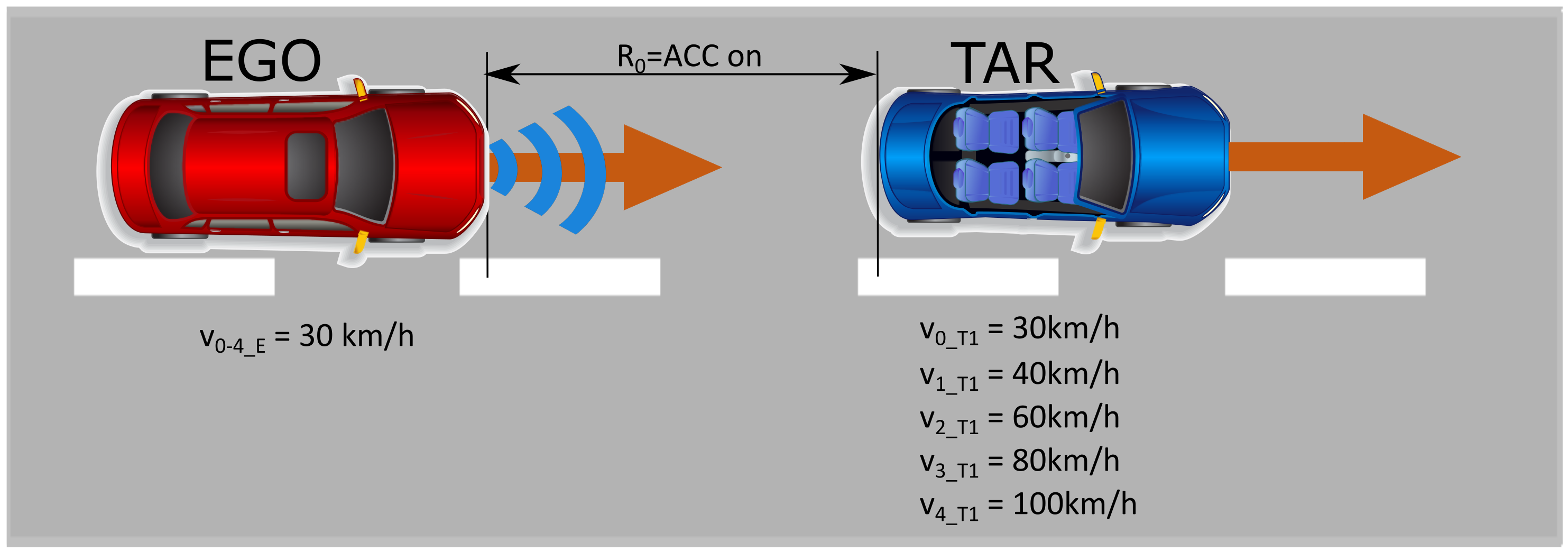
As more target vehicles were available, the manoeuvres were performed with up to five vehicles, with different configurations in terms of distance, speed and acceleration. For completeness, it should be mentioned that there were also manoeuvres involving up to 11 vehicles and two trucks, for which high accuracy GPS data are also available. In this research work, we demonstrate the potential of our assessing method using one selected manoeuvre—the Range test target leaving, which is depicted in Figure 2.
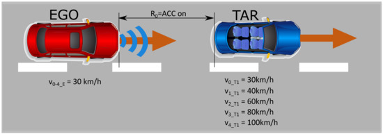
Figure 2.
Target leaving with constant delta speed.
This driving scenario contains four driving manoeuvres with varying target vehicle speed parameters. The initial state is defined as follows. Both vehicles with activated FSRA (Stop and Go ACC) and follow time set to the minimum reached the initial speed, which was set to 30 km/h for this manoeuvre. The distance to the TARGET vehicle controlled by the FSRA system of the EGO vehicle is in steady state condition. After the initial conditions are reached, the driver of the target vehicle changes the set speed of the FSRA system from the initial 30 km/h to vset_TAR = v1-4_TAR and leaves the EGO vehicle.
The measurement is considered complete when the distance between the vehicles has reached 250 m. To obtain the best measurement result, the angular orientation deviation (with respect to the direction of movement of the sensor) of the vehicles tested shall be kept below 1 degree. Unfortunately, the highway section used in this joint research project had a slightly curved characteristic, and therefore the angular orientation deviation continuously changes during the test runs and increases over 1 degree. This road geometry will lead to that the reflection points on a cumulative representation are shifted.
3.2.2. Vehicle Set-Up and Measurement System
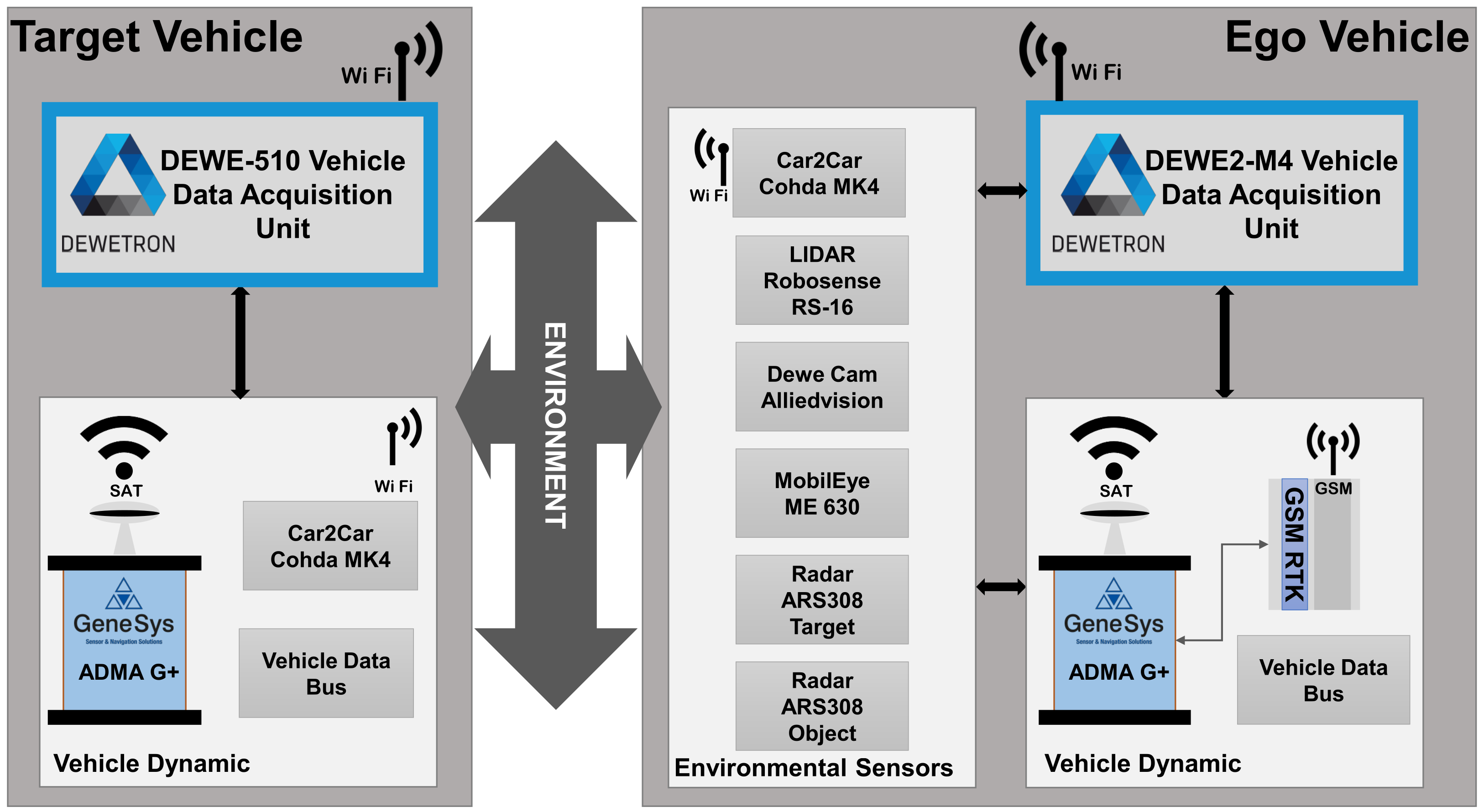
The sensor performance evaluation process is based on the comparison of low-level detection points from real measurements using automotive radar sensors and the corresponding simulation. This requires high accurate ground truth reference data of the environment including static and dynamic objects. An appropriate approach to generate ground truth data in terms of high accuracy measurements is illustrated in Figure 3.

Figure 3.
Schematic diagram of the measurement setup.
In order to detect as much information as possible of the surrounding of the car, the ego vehicle was equipped with the following sensors for environmental perception:
- Continental ARS 308 RADAR sensor configured to detect “targets”, also referred as low-level data and providing a new data set for each scan period.
- Continental ARS 308 RADAR sensor, configured to detect “objects” also referred to as highly processed data, provides information on the output of the tracking algorithm over several measurement periods.
- Robosense RS-16 LIDAR sensor, provides the data point cloud of the 360° sensor field of view.
- MobilEye ME-630 Front Camera Module, provides information of traffic signs, traffic participants, lane markings etc.
- Video Camera, provides visual information of the driving scenarios, used during post processing.
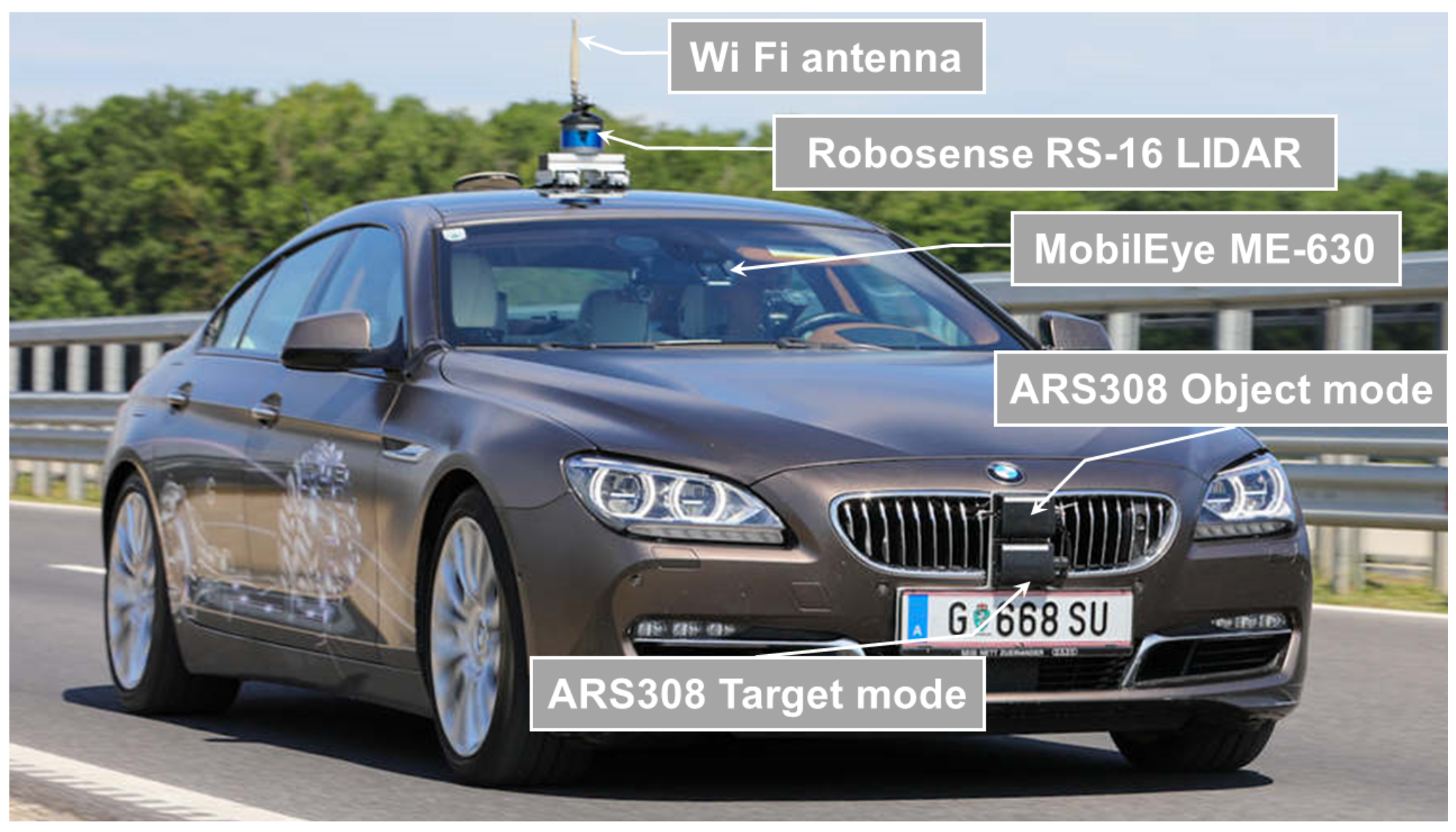
Radar sensors mounted on ego-vehicles are shown in Figure 4. In addition to the environmental sensors, the DEWETRON-CAPS Measurement System [28] was also mounted on the target and the ego vehicle. The CAPS measurement system allows the implementation of a wirelessly connected topology of data acquisition units, consisting of one master and several slave measurement PCs. In addition to the time-stamped input and output hardware interfaces, the core of the CAPS system is the high accuracy inertial measurement unit (IMU).
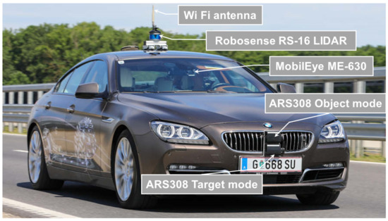
Figure 4.
Test vehicle measurement setup.
In our experimental setup, we used the most advanced Automotive Dynamic Motion Analyzer (ADMA-G-Pro+) GPS/INS-IMU from GeneSys Ltd. The ADMA, combined with an RTK-DGPS receiver [29] and connected to the Hungarian Positioning Service, provided high accuracy dynamic state and position information of the test vehicles in real time. In addition, an accurate time measurement is derived from the GPS/PPS signal, allowing synchronous measurement of all connected data acquisition units.
As all measurement inputs are time-stamped, the measurement system ensures that all data streams received local or via WLAN connection are stored in time synchronisation. In addition, the robust WLAN connection allows for the real-time transmission of dynamic state and position information from the target vehicle to the ego vehicle. The transmitted data allows the driver to monitor the driving scenario online to rapidly ensure the quality of the measurement process.
3.3. Re-Simulation of Experiments
When on-road measurements are conducted, it is possible to generate exact the same scenarios in the virtual simulation using the recorded trajectory of the vehicles. IPG CarMaker® was selected for the simulation environment, as this software package provides a Virtual Vehicle Environment (VVE), which represents a Multi-Body-Simulation (MBS). This includes the equations of motions, kinematics and also for ADAS applications, sensor models. For building a Digital-Twin of a highway section, a detailed Ultra-High-Definition (UHD) map was provided by Joanneum Research Forschungsgesellschaft, which were also a partner in the consortium [25]. This map represents a highly accurate representation of the highway section in an OpenDrive file format. As the road geometry in IPG CarMaker® [30] is defined in a RD5 file format, the UHD map in in OpenDrive format has to be converted.
The virtual map includes the following road geometry items [25]:
- lane borders and markings,
- lane centre lines,
- curbs and barriers,
- traffic signs and light pole and
- road markings.
This detailed description of the environment makes it possible to reduce deviations between the real and virtual world to a minimum. In addition to the preparation of the virtual environment, the recorded trajectories must be transformed from the geodetic WGS-84 coordinate system to a metric coordinate system, which is used in the simulation. Since the operating radius of the experiments is smaller than 50 km, the curvature of the earth can be neglected, and the transformation can be performed on a plane metric coordinate system, which is spanned relative to a reference point [28].
IPG CarMaker distinguishes between two categories of vehicles, the ego vehicle and traffic vehicle. The first one represents the Vehicle Under Test (VUT), including a multi-body representation where all sub-systems can be changed by the user, e.g., mounting ADAS sensors to the vehicle, whereas the traffic vehicle only represents a motion model, which is, in our case, a single-track model. In order to make the traffic vehicle follow the previously recorded and afterwards transformed trajectory, the exact position in x- and y-direction was given to the vehicle at every time step.
The ego vehicle is controlled via the IPG Driver, a mathematical representation of the behavior of a human. This Driver performs any interaction to the car, e.g., steering or accelerating/braking. If the ego vehicle is now given a target trajectory, this would be approximated by the IPG Driver, just as a human driver would do. However, since in our case, an exact following of the recorded trajectories is absolutely necessary for the evaluation of the sensor model, a by-pass has to be performed on the driver model. This was done with a modification in the C-Code interface provided by the software vendor IPG. With this adaptation, the ego vehicle is now able to reproduce the same trajectory in the virtual environment as it was measured in the real world, ignoring any intervention by the IPG driver.
For the replay of the scenarios, a standard IPG-Car parameter set was used, including models of powertrain, tires, chassis, steering, aerodynamics and sensors. Since the ego vehicle exactly follows the recorded trajectory, no detailed parameter setting is required. The simulation software offers a number of different sensor models, which operate at different levels, ranging from ideal sensors to phenomenological sensors and to raw signal interfaces.
Since this paper focuses on the validation of low-level sensor models, the RSI radar-sensor model from IPG CarMaker V 8.1.1® [30] is considered and described in detail.
3.3.1. IPG RSI Radar Sensor Model
This sensor model provided by IPG CarMaker imitates the physical wave propagation by an optical ray-tracing approach. It includes the major effects of wave propagation, e.g.,
- Multipath/repeated path propagation.
- Relative Doppler shift.
- Road clutter.
- False positive/negative detections of targets.
Using this ray optical sensor model in a virtual environment requires the modelling of material properties of objects, such as the relative electric permittivity for electromagnetic waves and scattering effects. This parameters have a significant influence on the reflected direction and field strength of the reflected wave. The reflections are created by a detailed 3D surface in the visualisation. In the used set-up, the default values provided by the simulation tool for a 77 GHz radar were used.
3.3.2. Parameter Setting of the Sensor Model
Radar sensors are influenced by a multitude of parameters, which makes the parameter setting of such models complex. To ensure the comparability of the sensor model, the real hardware was treated like a black box so the sensor model was set with those parameters given in the data sheet provided by the manufacturer of the Radar sensor. To set the parameters for the atmospheric environment, temperatures and and in particular the data sheet based parameters: Field of View, Range, Cycle time, Max. Channels, Frequency, Separability Distance, Separability Azimuth, Separability Elevation, and Separability Speed was used.
With the additional offered two “design” parameters and scattering effect, CarMaker® gives users the possibility to fine tune the sensor model. However, one parameter given in the data sheet of the real hardware was not adjustable in the software package. The inaccuracy depending on the distance of the detected object was afterwards superimposed to the simulation results, as this leads to more robust results. To make this modified data visible in the results, this data is marked as modified data in Section 4 [30,31].
3.4. Labelling of Radar Measurement Data
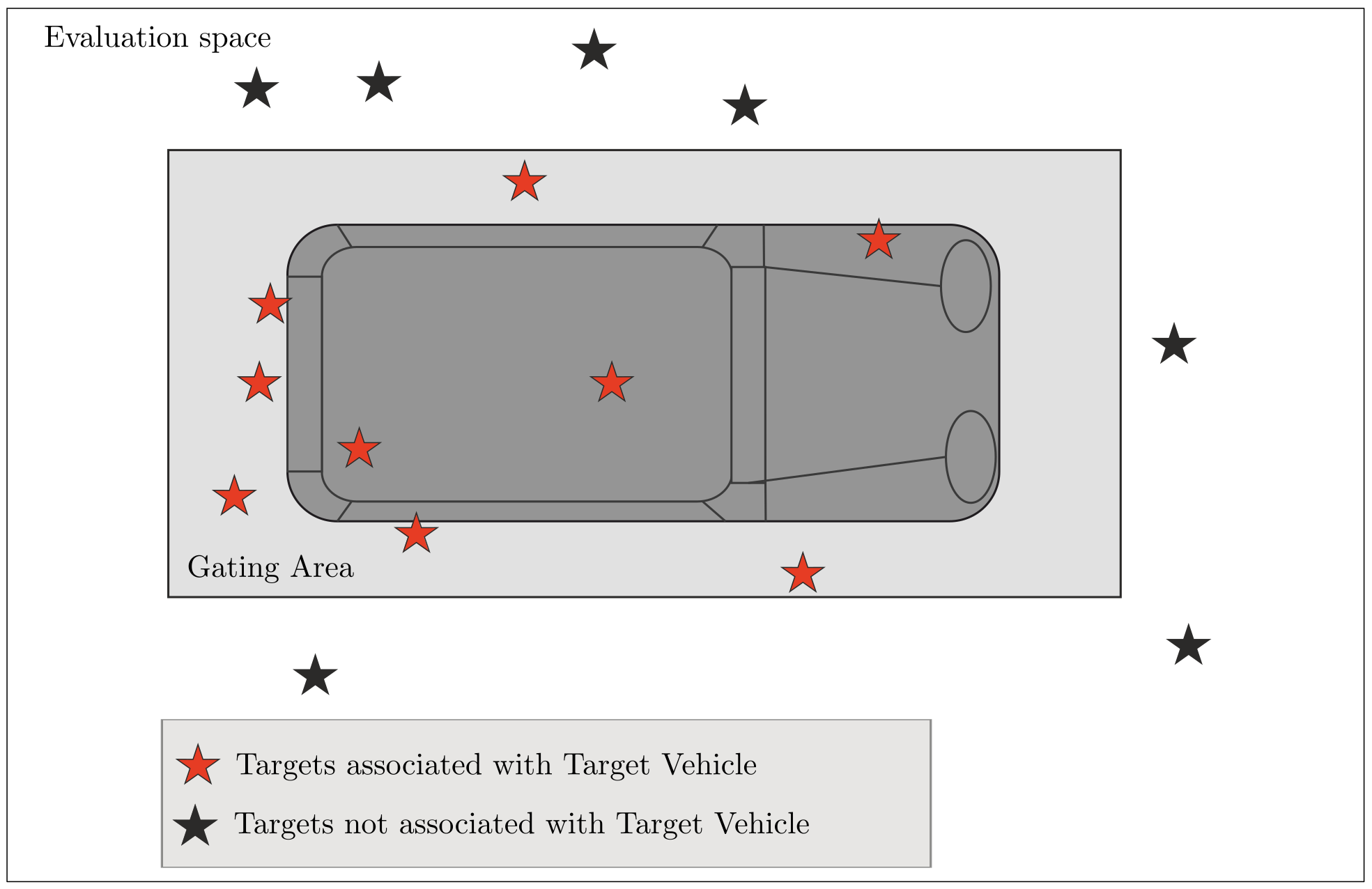
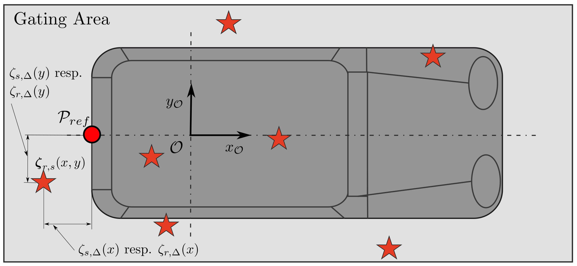
In order to assign the individual reflection points of the radar sensor to the dynamic targets, a method that is already known in the field of object tracking is used, namely the gating technique. Using the ground truth information of the dynamic objects, target points only in a specific shaped area around an object of interest are considered. Figure 5 represents the gating area with the associated and not associated target points. The shape of the gating area can be variously designed, such as rectangular or elliptical [32].

Figure 5.
Gating area of the target vehicle with and with not associated reflection points according to [31].
In accordance with the shape of an average car, we used a rectangular shape. In this case, only dynamic objects are considered, as no static object information is available in the virtual map, e.g., bridge heads or overhead traffic signs. This means that the evaluation is limited to moving objects where the ground truth is measured with the RTK-GPS IMU measurement equipment but is also applicable to static objects, given that the ground truth is referenced.
3.5. Evaluation Procedure
Different evaluation metrics are given in literature, such as comparison of occupancy grid maps, statistical hypothesis testing, confidence intervals, correlation measurements and the generation of probability density functions [18,21,33,34]. In contrast to object list based deterministic sensor models, physical non-deterministic sensor models do not allow a direct comparison between experimental observations and simulation models. To make the highly stochastic process of a physical radar-sensor model comparable, including the physical attributes, e.g., the relative velocity or RCS value, statistical evaluation methods are best suited to describe the distribution of parameters in space and time.
Using previously labelled data, it is possible to evaluate them by statistical means in such a way that a quantitative statement can be made about the quality of the sensor model used in comparison to the real hardware. Introducing a reference point on the target vehicle enables the calculation of the deviation on every radar detection point to the ground truth of the dynamic object, see Figure 6. Radar detection points are represented by the vector for the measured sensor data and for the simulated data. The deviation is calculated with
where representing the deviation of the simulation data and representing the deviation of the real sensor data to the reference point.

Figure 6.
Reference point on the dynamic object; Deviation target points real sensor to reference point and deviation target points simulation to reference point according to [31].
Assuming radar sensors are subject to a highly stochastic process, the detection points can be treated as realizations of a distribution function [35], p. 35. Using methods, including kernel density estimation (KDE), a probability density function (PDF) can be generated from the large number of realizations.
3.6. Validation Metrics for Comparing Probability Distributions
The validation of simulation models is based on the numerical comparison of data sets from experimental observations and the computational model output for a given use case. To quantify the comparison, validation metrics can be defined to measure the difference between the physical observation and the simulated output. Whether comparing measured physical quantities or virtual simulations, observed values contain uncertainties. In the presence of uncertainties, the observed values subject to validation are samples from a distribution of possible measured values, which are usually unknown.
To optimally quantify the difference or the similarity between distributions, we need the actual distributions. For the empirical data sets resulting from experimental observations (real radar sensor) and the output of the computational model (physical radar-sensor model), we do not know the actual distribution, or even its shape. Although one can always make assumptions (parametric) or estimate kernel density estimates (KDE), these are not quite ideal in practice, as their analysis is limited to specific types of distributions or kernels used. To stay as close to the data as possible, we therefore consider a non-parametric divergence measure. Non-parametric models are extremely useful when moving from discrete data to probability functions or distributions.
Non-parametric approaches are another way to estimate distributions. Such methods can be used to map discrete distributions of any shape. The simplest implementation of non-parametric distribution estimation is the histogram. Histograms benefit from knowledge of the data sets to be estimated and require fine-tuning to achieve optimal estimation results. In our application, this knowledge is available, since the bin width of the histogram can be determined according to the real sensor data sheet.
As stated above, a metric is a mathematical operator that gives a formal measure of the difference between experimental and model results. The metric plays a central role as it can be used to describe the fidelity of sensor models used to validate ADAS/AD functions. A low metric value means a good match and vice versa. According to [18] the metric can be defined by the following criteria: it must be intuitively understandable, applicable to both deterministic and non-deterministic data, a good metric defines a confidence interval as a function of the number of measured data and meet the mathematical properties of the metric.
The variables measured by perception sensors are usually non-parametric due to the highly stochastic nature of the output data [24]. Based on these properties, one possible description of the correspondence between synthetic and real perceptual data could be the comparison of their probability distribution functions. In the context of validating perception–sensor models, the most useful characterization appears to be the comparison of the distributions of random variables and the shapes of the corresponding observations. Random variables whose distribution functions are the same are called “distribution inequalities”.
If the shapes of the distributions are not exactly the same, the difference can be measured using several possible measures. Maupin et al. [36] described a number of validation metrics for deterministic and probabilistic data that are used to validate computational models by quantifying the information provided by physical and simulated observations. In the context of this research, we proposed to use the Jensen–Shannon Divergence (JSD) [37], as it provides a quantified expression of the results of a comparison between two or more discrete probability distributions in a normalised manner.
The JSD, is a symmetrised version of the Kullback–Leibler Divergence described in detail in [18,36]. We consider a true discrete probability distribution and its approximation over the values taken on by the random variable. The Jensen–Shannon Divergence calculated with
where is the mean distribution for and , as given by
The Jensen–Shannon Divergence uses the Kullback–Leibler Divergence to calculate a normalized measure. If and describe the probability distribution of two discrete random variables, the KL divergence is calculated according to Equation (5).
Since the JS Divergence is a smoothed and normalised measure from the KL Divergence, it can be easily integrated into development processes. By definition, the square root of the Jensen–Shannon divergence describes the Jensen–Shannon distance.
As both the divergence DJS and the distance DistJS are symmetric with respect to the arguments and and the JS-Divergence is always non-negative, the value of DJS is always a real number in the closed interval of [0; 1].
If the value is 0, the two distributions and are the same, if the value is 1, the two distributions are as different as possible. For better interpretation we present JSD in percentage values in the following. As DistJS fulfils the mathematical properties of a true metric [38], such as symmetry, triangle inequality and identity, the Jensen–Shannon Distance is a valid metric distance.
4. Results
In this chapter, the results of the statistical analysis are presented, showing the behaviour and the differences of the sensor model compared to the Ground Truth and the real sensor. In order to implement the DGT-SMV procedure and to illustrate the potential of the method, the driving scenario defined in Section 3.2.1 was used. As already described in Section 3.3.2, the modified data set with the super-positioned deviation was used for the evaluation of the RSI sensor model.
The data of both, the real and the simulated radar sensor, was accordingly to the radar properties split in a near range (0 to 60 m) and a far range (60 to 200 m) section. The used radar sensor can detect objects in the near range between 0 and 60 m in near and far range mode, which results in an overlap of the two sensor modes. For this reason, the far range was further subdivided into those data from the 0 to 60 m and 60 to 200 m for detailed analysis.
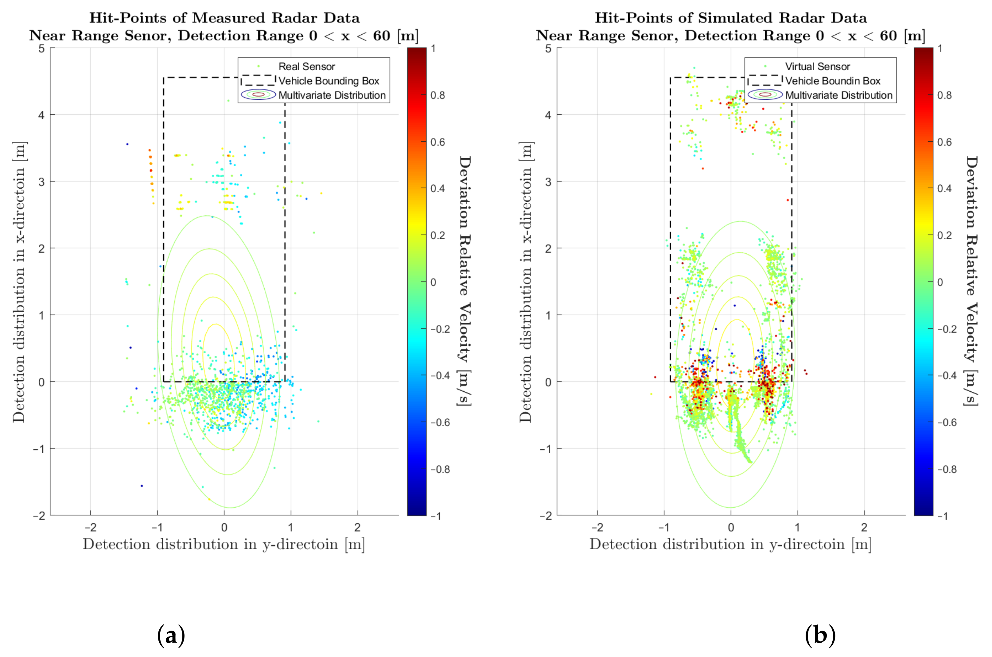
4.1. Comparison of Simulated and Measured Radar Signals
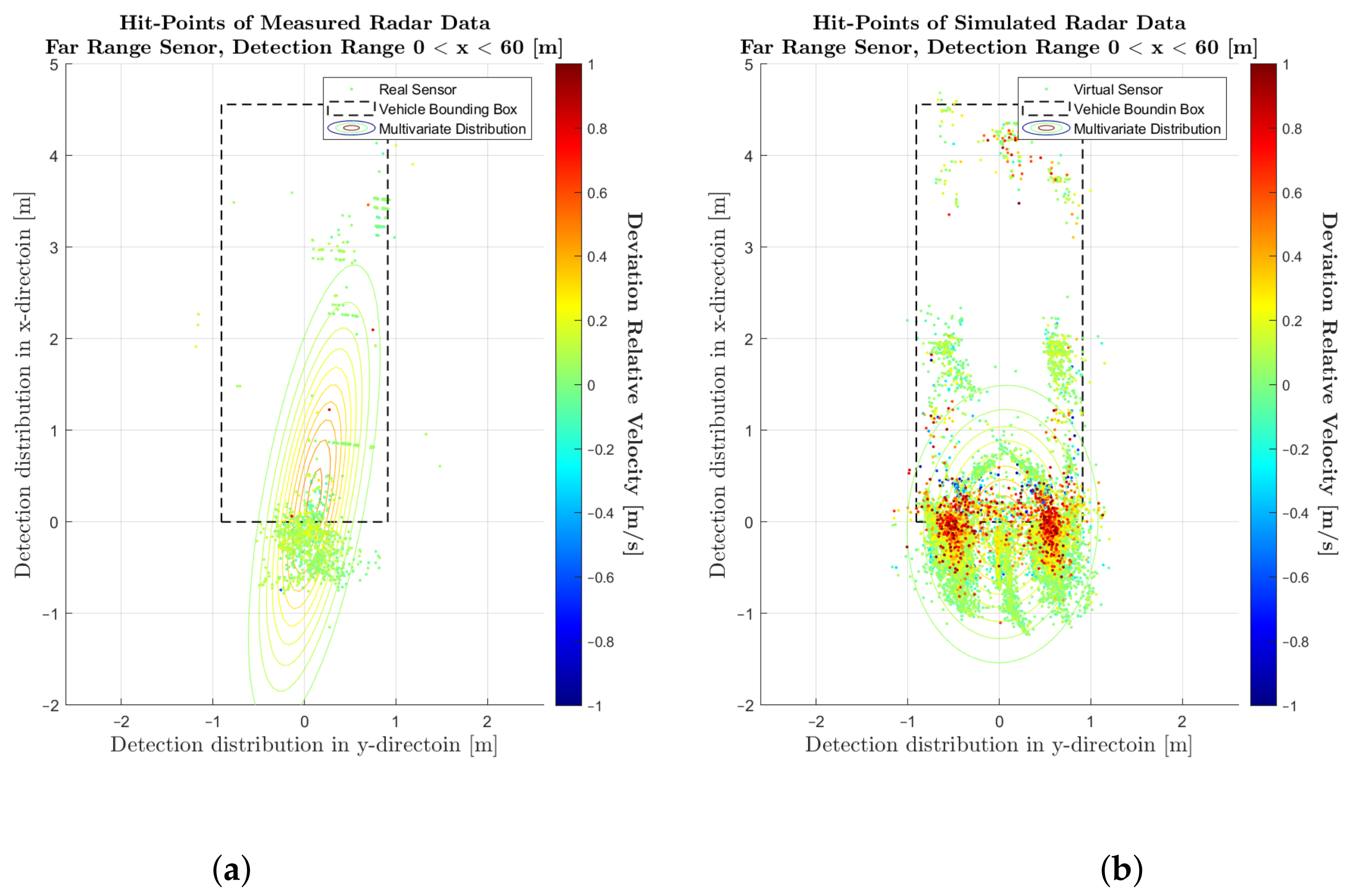
In Figure 7, Figure 8 and Figure 9, visualizations of various statistical analysis of the near range radar and radar model are shown. Figure 7a,b presents the visualization of the radar detection points, which are associated to the corresponding dynamic target. The grey scale of each target point indicates its relative velocity, and the stroked line indicates the bounding box of the target vehicle. The contour lines in this plots are representing the multi-variant distribution of the reflection points. In Figure 8, the PDF’s of the deviation to the reference point in x- and y-direction of the realizations are shown.

Figure 7.
Evaluation of the detections in the range of 0 to 60 m of the near-range radar sensor and sensor model. (a) Scatterplot of detections for the real sensor. (b) Scatterplot of detections for the sensor model.

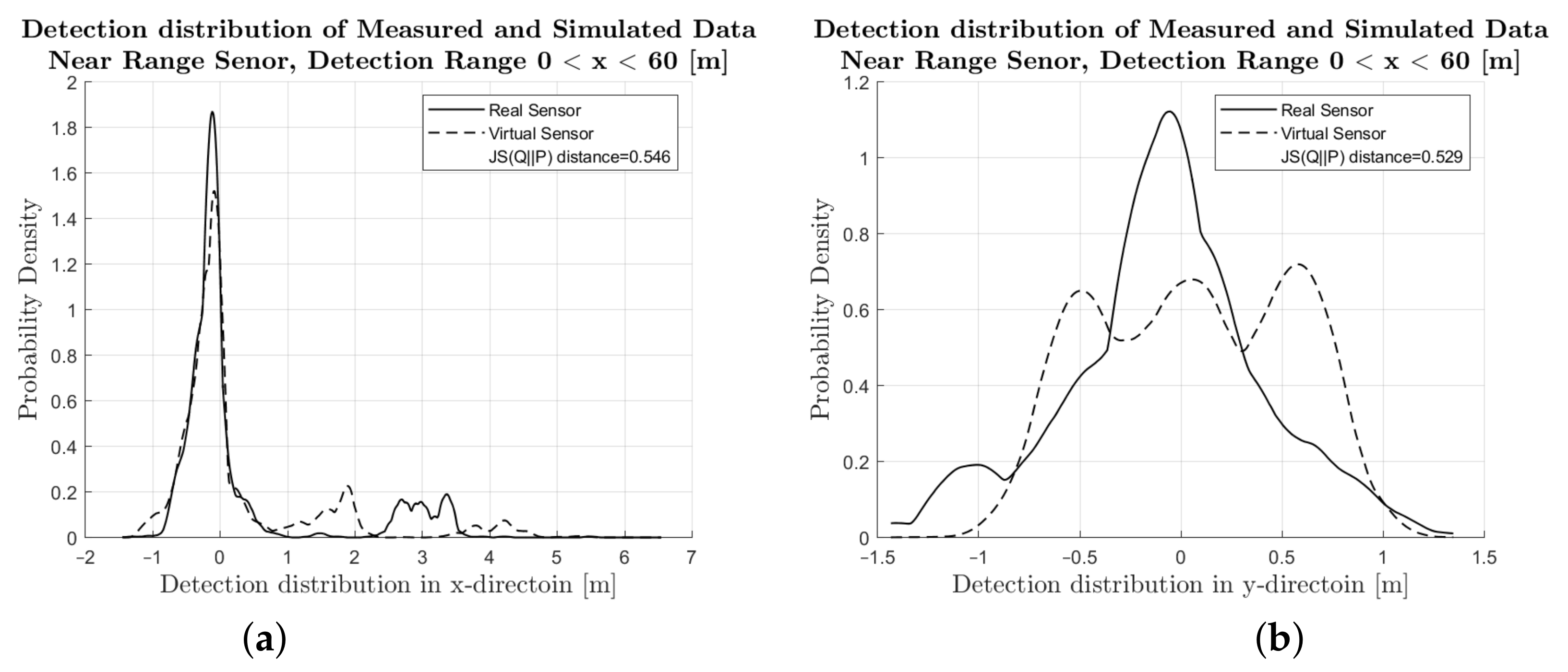
Figure 8.
Evaluation of the detections in the range of 0 to 60 m of the near-range radar sensor and sensor model. (a) PDF of the deviation in the x-direction from of the real sensor and sensor model. (b) PDF of the deviation in the y-direction from of the real sensor and sensor model.

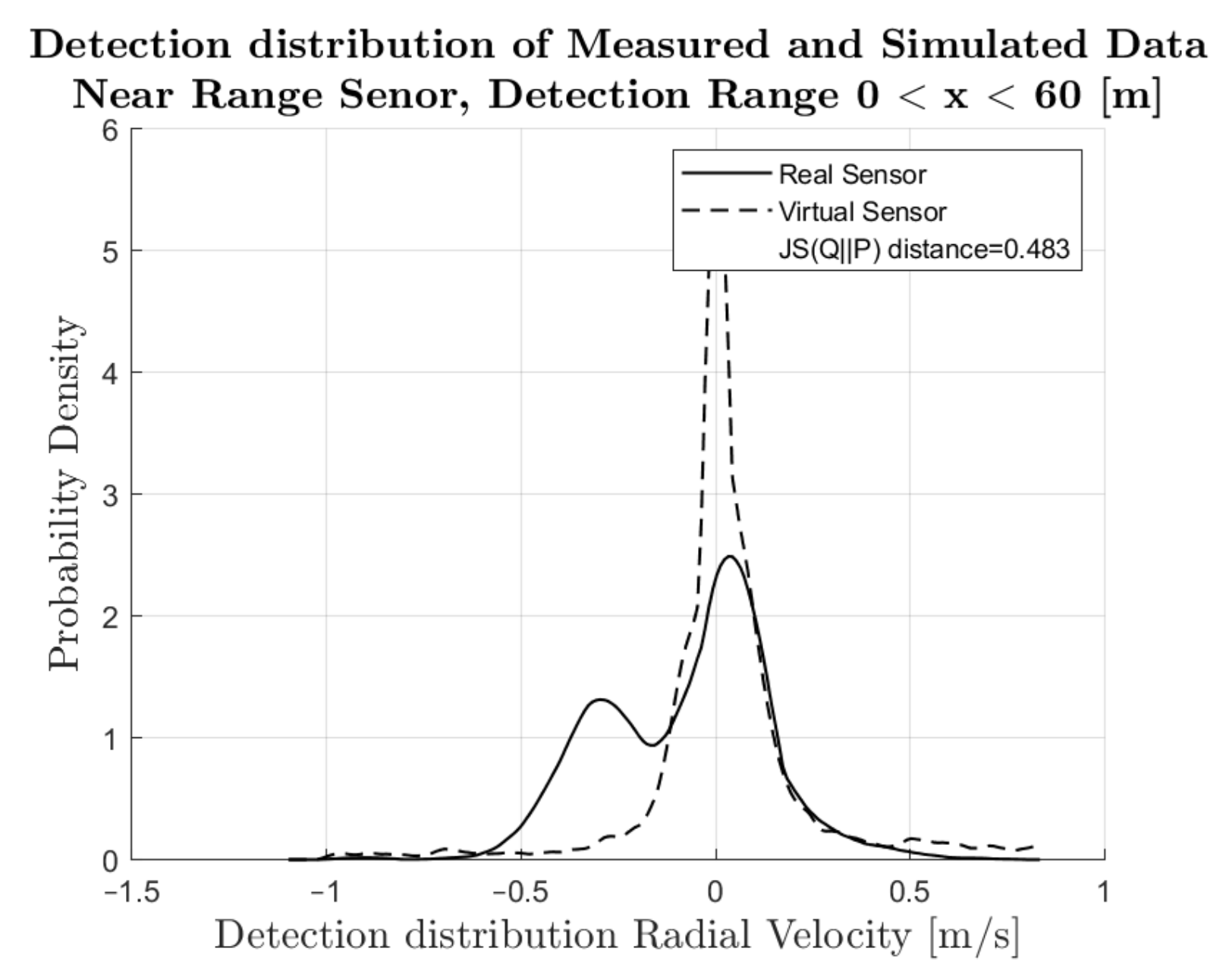
Figure 9.
Evaluation of the detections in the range from 0 to 60 m of the near-range radar sensor and sensor model: PDF of the relative velocity in the x-direction from the reference velocity of the real sensor and sensor model.
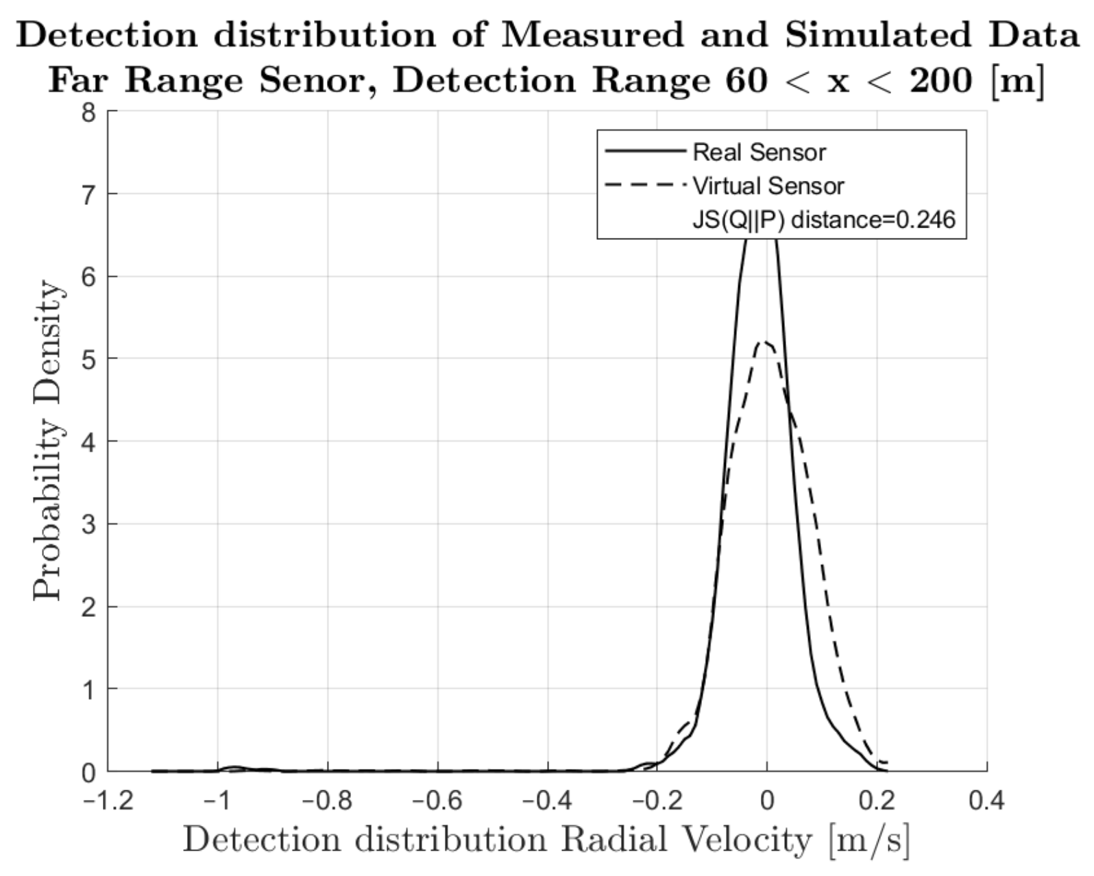
The probability distribution can not only be used for the qualitative assessment of the distribution of the reflections but also serves as a basic prerequisite for the calculation of the Jensen–Shannon divergence. In Figure 8a, the deviation in the longitudinal direction, and in Figure 8b, the deviation in the lateral direction is shown. Figure 9 shows a PDF of the deviation of the relative velocity of each radar detection point in comparison to the Ground Truth relative velocity of the target vehicle.
In Figure 10, Figure 11 and Figure 12, the visualization of the statistical analysis of the far range sensor in the near range section are shown. The results of the far range sensor for the far range section (60 to 200 m) can be found in Figure A1, Figure A2, Figure A3.

Figure 10.
Evaluation of the detections in the range of 0 to 60 m of the far-range radar sensor and sensor model. (a) Scatterplot of detections of the real sensor. (b) Scatterplot of detections of the sensor model.
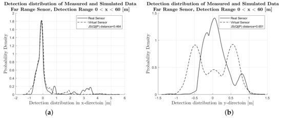
Figure 11.
Evaluation of the detections in the range of 0 to 60 m of the far-range radar sensor and sensor model. (a) PDF of the deviation in the x-direction from of the real sensor and sensor model. (b) PDF of the deviation in the y-direction from of the real sensor and sensor model.
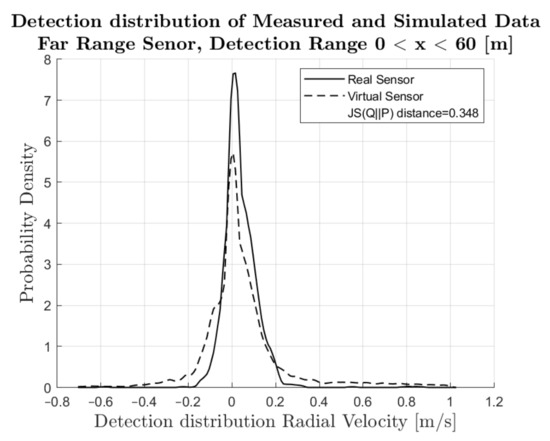
Figure 12.
Evaluation of the detections in the range of 0 to 60 m of the far-range radar sensor and sensor model: PDF of the relative velocity in the x-direction from the reference velocity of the real sensor and sensor model.
4.2. Performance Metrics
When evaluating the performance of a virtual sensor for accuracy or fidelity, the correct performance metric should be selected to meet the requirements of the application. As described in [36], the data sets under comparison can be treated with or without uncertainty. Since, in our application, both experimental and predicted values are treated with uncertainty, comparison in the shape of a non-parametric discrete distribution is one promising solution.
The Jensen–Shannon Divergence (JSD) measures the distance between two discrete distributions by comparing the shape of two PDFs, one of which is the accuracy reference (real sensor data) and the other the output of a virtual model. JSD has two important features: first, JSD includes all the statistical information known about each distribution in the comparison. This means that the comparison is not limited to the average behaviour of the distributions. Second, it provides a real mathematical metric.
Since the Jensen–Shannon distance is a real mathematical metric, using the property that the value of DistJS is always a real number in the closed interval between 0 and 1, and if the value is 0, then the two distributions, and , are the same; otherwise they differ as much as possible, a quantitative comparison can be made between the sets of simulation.
In Table 2, Table 3 and Table 4, the JSD is expressed as a percentage for the near range as well as for the far range. The evaluated variables are , defining the JSD metric for the relative distance in x, , for the relative distance in y and for the relative velocity v.
Table 2.
The results for the near-range radar sensor, detection range 0 < x < 60 [m].
Table 3.
The results for the far-range radar sensor, detection range 0 < x < 60 [m].
Table 4.
The results for the far-range radar sensor, detection range 60 < x < 200 [m].
5. Discussion
Inspecting the results, a quick overview on the performance of the virtual sensor can immediately be achieved by the JSD metrics, where, for the deviations , 0% is perfect performance and 100% is the worst performance. In our example, it can be seen that, in the far range, the virtual sensor is more accurate in reproducing the relative velocity than in the relative distance. For the relative velocity, the JSD of is 34.2% up to 60 m and 25.6% up to 200 m. In the near range, the performance is worse at 51%.
For the relative distance, the better performance is seen in the x direction. The JSD of is 46.5% in the far range up to 60 m and 44.1% up to 200 m, for the near range 54.8% was observed. In the y direction, the related JSD values of are 65.1%, 52.8% and 53.1%, respectively.
This result is confirmed by visual inspection of the PDF illustrated in Figure 8, Figure 9, Figure 11 and Figure 12 as well as the scatter plots in Figure 7 and Figure 10. Comparing the shape of the PDFs, the strengths and shortcomings of the sensor model can be assessed, providing recommendations for parameter tuning and drawing conclusions on the validity of the results. The explanation of the results may be found in the specific modelling approach of the commercial radar-sensor model and is not part of this paper.
Limitations
The paper is subject to the following limitations:
- Limitations for dynamic objects: Since the UHD map in the simulation did not include any static objects, such as bridges, traffic signs, roadside barriers, vegetation and others, we only focused on the dynamic objects. The method can be enhanced for static objects in case the ground truth is annotated in the virtual sensor data.
- Limitations for the investigated radar phenomena: Here, we focused on a specific radar related phenomenon, the rapid fluctuation of the measured RCS over azimuth angles. Other phenomena as described in [26], such as multipath-propagation and separability were not covered here, since the real world driving tests included some limitations detected afterwards. The method can be extended to other phenomena, one has to define suitable driving scenarios and performance criteria.
- Limitations of specific benchmark results: Since no parameter tuning was performed in the IPG RSI model, the results obtained are not a direct indicator of the capabilities of the sensor model. However, the method can be used to improve the quality of the modelling by fine-tuning the model parameters. Only after finding the best fit does the quality assessment become complete and can be directly compared with another model.
- Limitations for vehicle contours: According to the literature, the Jensen–Shannon divergence can be extended to a multivariate space with independent components, which allows for the comparison of multivariate random variables, making it possible to consider the contour of the vehicle. However, in this paper, we focused on the development of the methodology and data where the results are based on included one type of target vehicle. Hence, the difference of the rear wall of different vehicles can not be explicitly taken into account.
These limitations will be addressed in future research.
6. Summary
Despite the advantages of automated driving technologies with respect to safety, comfort, efficiency and new forms of mobility, only driver assistance of SAE levels 0 to 2, with the first applications in SAE L3, are on the market. One of the main reasons is the lack of proof in functional safety, which is due to the immense efforts required in real world testing. Virtual testing and validation is a promising option; however, the proof of realism of the simulation is not guaranteed at the moment.
One of the main obstacles is to reproduce the performance of machine perception in the simulation. Currently, there is a huge amount of development and research ongoing in providing virtual sensors. However, there is no accepted method for the proof of realism and prognosis quality for sensor models. In the present paper, we developed a method, the Digital Ground Truth–Sensor Model Validation (DGT-SMV), which is based on the re-simulation of actual test drives to thus allow for a direct comparison between the simulated and recorded sensor output. This approach requires defining suitable driving manoeuvres to reproduce the individual phenomena of the real sensor.
For the radar sensor, this is the multipath-propagation, separation ability and rapid fluctuation of the measured RCS over azimuth angles. The approach also requires accurate measurement equipment that records the ground truth of the driving scenario synchronously to the sensor data. After labelling the ground truth of the sensor output, a direct comparison between the simulated and recorded sensor output is possible.
For performance evaluation, we proposed a visual inspection of the simulated and recorded sensor output that we call scatter plots and, secondly, the transformation of these data with statistical methods based on Probability Distribution Functions to reveal the main performance of the virtual sensors. Finally, for a quick quantitative comparison, we proposed performance metrics based on the Jensen–Shannon distance. The method was applied on a commercially available sensor model (RSI radar-sensor model of IPG CarMaker) using real test drives on a closed highway in Hungary. For those tests, a high precision digital twin of the highway was available as well as the ground truth of the moving objects using RTK-GPS localization.
The results show that the DGT-SMV method is a promising solution for performance benchmarks of low-level radar-sensor models. In addition, the method can also be transferred to other active sensor principles, such as lidar and ultrasonic sensors.
Author Contributions
Conceptualization, Z.F.M.; methodology, Z.F.M.; software, C.W., P.L. and Z.F.M.; validation, Z.F.M. and C.W.; formal analysis, Z.F.M. and C.W.; investigation, Z.F.M. and C.W.; resources, V.R.T., A.E. and P.L.; data curation, Z.F.M. and C.W.; writing–original draft preparation, Z.F.M., C.W. and A.E.; writing–review and editing, Z.F.M., C.W. and A.E.; visualization, Z.F.M. and C.W.; supervision, A.E.; project administration, A.E. and V.R.T. All authors have read and agreed to the published version of the manuscript.
Funding
This research was not externally funded, however the preparatory work and the collection of measurement data was done in the funded Central System project, (2020-1.2.3-EUREKA-2021-00001) and received funding from the NRDI Fund by the National Research, Development and Innovation Office Hungary. Open Access Funding by the Graz University of Technology.
Data Availability Statement
Data and software used here are proprietary and cannot be released.
Acknowledgments
The authors would like to express their thanks to the availability of measurement data as published in [25] and those who have supported this research and to the Graz University of Technology also.
Conflicts of Interest
The authors declare no conflict of interest.
Appendix A

Figure A1.
Evaluation of the detections in the range of 60 to 200 m of the far-range radar sensor and sensor model. (a) Scatterplot of the real sensor detections. (b) Scatterplot of the sensor model detections.
Figure A1.
Evaluation of the detections in the range of 60 to 200 m of the far-range radar sensor and sensor model. (a) Scatterplot of the real sensor detections. (b) Scatterplot of the sensor model detections.
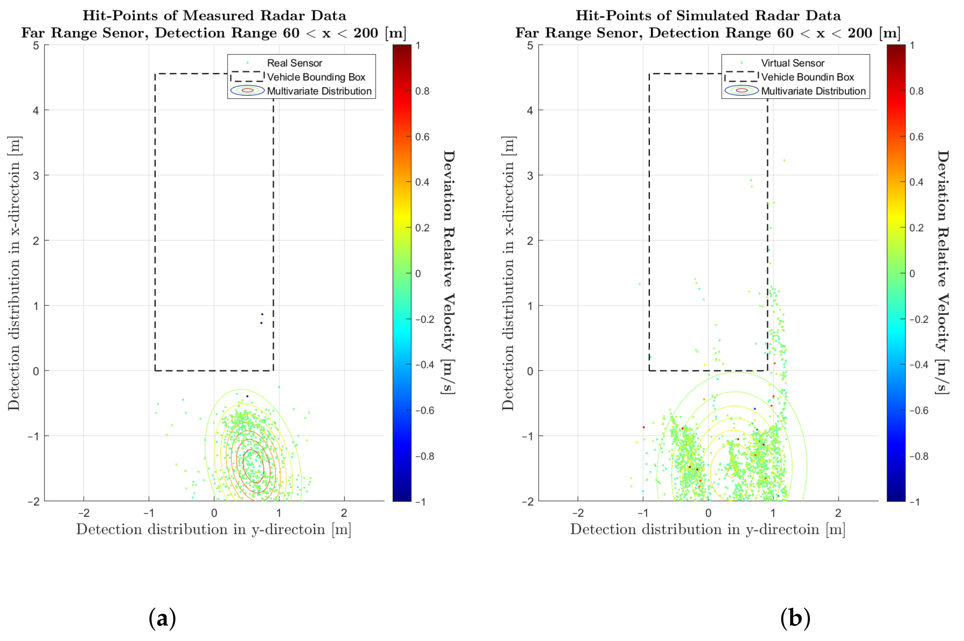

Figure A2.
Evaluation of the detections in the range of 60 to 200 m of the far-range radar sensor and sensor model. (a) PDF of the deviation in the x-direction from of the real sensor and sensor model. (b) PDF of the deviation in the y-direction from of the real sensor and sensor model.
Figure A2.
Evaluation of the detections in the range of 60 to 200 m of the far-range radar sensor and sensor model. (a) PDF of the deviation in the x-direction from of the real sensor and sensor model. (b) PDF of the deviation in the y-direction from of the real sensor and sensor model.
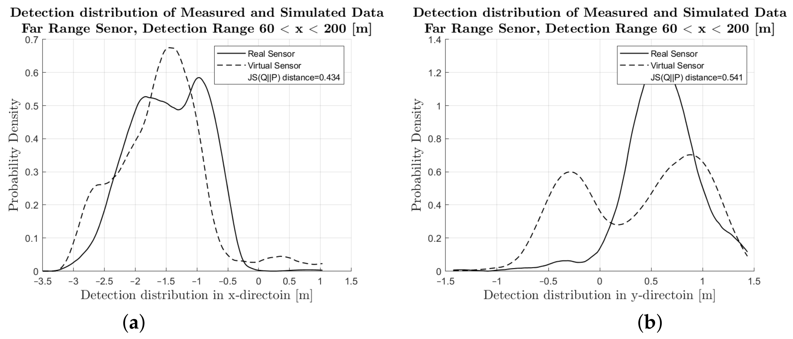

Figure A3.
Evaluation of the detections in the range of 60 to 200 m of the far-range radar sensor and sensor model: PDF of the relative velocity in the x-direction from the reference velocity of the real sensor and sensor model.
Figure A3.
Evaluation of the detections in the range of 60 to 200 m of the far-range radar sensor and sensor model: PDF of the relative velocity in the x-direction from the reference velocity of the real sensor and sensor model.
References
- Soteropoulos, A.; Pfaffenbichler, P.; Berger, M.; Emberger, G.; Stickler, A.; Dangschat, J.S. Scenarios of Automated Mobility in Austria: Implications for Future Transport Policy. Future Transp. 2021, 1, 747–764. [Google Scholar] [CrossRef]
- DESTATIS. Verkehr. Verkehrsunfälle. In Technical Report Fachserie 8 Reihe 7; Statistisches Bundesamt: Wiesbaden, Germany, 2020; p. 47. [Google Scholar]
- Dingus, T.A.; Guo, F.; Lee, S.; Antin, J.F.; Perez, M.; Buchanan-King, M.; Hankey, J. Driver crash risk factors and prevalence evaluation using naturalistic driving data. Proc. Natl. Acad. Sci. USA 2016, 113, 2636–2641. [Google Scholar] [CrossRef] [PubMed] [Green Version]
- Tirachini, A.; Antoniou, C. The economics of automated public transport: Effects on operator cost, travel time, fare and subsidy. Econ. Transp. 2020, 21, 100151. [Google Scholar] [CrossRef]
- Winner, H.; Hakuli, S.; Lotz, F.; Singer, C. (Eds.) Handbuch Fahrerassistenzsysteme: Grundlagen, Komponenten und Systeme für Aktive Sicherheit und Komfort; ATZ-MTZ-Fachbuch Book Series; Springer: Berlin/Heidelberg, Germany, 2015. [Google Scholar]
- Kalra, N.; Paddock, S.M. Driving to safety: How many miles of driving would it take to demonstrate autonomous vehicle reliability? Transp. Res. Part A Policy Pract. 2016, 94, 182–193. [Google Scholar] [CrossRef]
- Szalay, Z. Next Generation X-in-the-Loop Validation Methodology for Automated Vehicle Systems. IEEE Access 2021, 9, 35616–35632. [Google Scholar] [CrossRef]
- Yonick, G. New Assessment/Test Method for Automated Driving (NATM): Master Document (Working Documents). 2021. Available online: https://unece.org/sites/default/files/2021-04/ECE-TRANS-WP29-2021-61e.pdf (accessed on 18 January 2022).
- ISO 26262-2:2018; Road Vehicles—Functional Safety—Part 2: Management of Functional Safety. International Standardization Organization: Geneva, Switzerland, 2018.
- Schlager, B.; Muckenhuber, S.; Schmidt, S.; Holzer, H.; Rott, R.; Maier, F.M.; Saad, K.; Kirchengast, M.; Stettinger, G.; Watzenig, D.; et al. State-of-the-Art Sensor Models for Virtual Testing of Advanced Driver Assistance Systems/Autonomous Driving Functions. SAE Int. J. Connect. Autom. Veh. 2020, 3, 233–261. [Google Scholar] [CrossRef]
- Cao, P.; Wachenfeld, W.; Winner, H. Perception–sensor modeling for virtual validation of automated driving. IT Inf. Technol. 2015, 57, 243–251. [Google Scholar] [CrossRef]
- Chen, S.; Chen, Y.; Zhang, S.; Zheng, N. A Novel Integrated Simulation and Testing Platform for Self-Driving Cars With Hardware in the Loop. IEEE Trans. Intell. Veh. 2019, 4, 425–436. [Google Scholar] [CrossRef]
- Yeong, D.J.; Velasco-Hernandez, G.; Barry, J.; Walsh, J. Sensor and Sensor Fusion Technology in Autonomous Vehicles: A Review. Sensors 2021, 21, 2140. [Google Scholar] [CrossRef] [PubMed]
- Safety First for Automated Driving. 2019. Available online: https://group.mercedes-benz.com/dokumente/innovation/sonstiges/safety-first-for-automated-driving.pdf (accessed on 3 March 2022).
- Maier, M.; Makkapati, V.P.; Horn, M. Adapting Phong into a Simulation for Stimulation of Automotive Radar Sensors. In Proceedings of the 2018 IEEE MTT-S International Conference on Microwaves for Intelligent Mobility (ICMIM), Munich, Germany, 15–17 April 2018; pp. 1–4. [Google Scholar] [CrossRef]
- Slavik, Z.; Mishra, K.V. Phenomenological Modeling of Millimeter-Wave Automotive Radar. In Proceedings of the 2019 URSI Asia-Pacific Radio Science Conference (AP-RASC), New Delhi, India, 9–15 March 2019; pp. 1–4. [Google Scholar] [CrossRef]
- Cao, P. Modeling Active Perception Sensors for Real-Time Virtual Validation of Automated Driving Systems. Ph.D. Thesis, Technische Universität, Darmstadt, Germany, 2018. [Google Scholar]
- Schaermann, A. Systematische Bedatung und Bewertung Umfelderfassender Sensormodelle. Ph.D. Thesis, Technische Universität München, München, Germany, 2019. [Google Scholar]
- Gubelli, D.; Krasnov, O.A.; Yarovyi, O. Ray-tracing simulator for radar signals propagation in radar networks. In Proceedings of the 2013 European Radar Conference, Nuremberg, Germany, 9–11 October 2013; pp. 73–76. [Google Scholar]
- Anderson, H. A second generation 3-D ray-tracing model using rough surface scattering. In Proceedings of the Vehicular Technology Conference, Atlanta, GA, USA, 28 April–1 May 1996; pp. 46–50. [Google Scholar] [CrossRef]
- Sargent, R.G. Verification and validation of simulation models. In Proceedings of the 2010 Winter Simulation Conference, Baltimore, MD, USA, 5–8 December 2010; pp. 166–183. [Google Scholar] [CrossRef] [Green Version]
- Oberkampf, W.L.; Trucano, T.G. Verification and validation benchmarks. Nucl. Eng. Des. 2008, 238, 716–743. [Google Scholar] [CrossRef] [Green Version]
- Roth, E.; Dirndorfer, T.J.; von Neumann-Cosel, K.; Gnslmeier, T.; Kern, A.; Fischer, M.O. Analysis and Validation of Perception Sensor Models in an Integrated Vehicle and Environment Simulation. In Proceedings of the 22nd International Technical Conference on the Enhanced Safety of Vehicles, Washington, DC, USA, 13–16 June 2011. [Google Scholar]
- Holder, M.; Rosenberger, P.; Winner, H.; D’hondt, T.; Makkapati, V.P.; Maier, M.; Schreiber, H.; Magosi, Z.; Slavik, Z.; Bringmann, O.; et al. Measurements revealing Challenges in Radar Sensor Modeling for Virtual Validation of Autonomous Driving. In Proceedings of the 2018 21st International Conference on Intelligent Transportation Systems (ITSC), Maui, HI, USA, 4–7 November 2018; pp. 2616–2622. [Google Scholar] [CrossRef] [Green Version]
- Tihanyi, V.; Tettamanti, T.; Csonthó, M.; Eichberger, A.; Ficzere, D.; Gangel, K.; Hörmann, L.B.; Klaffenböck, M.A.; Knauder, C.; Luley, P.; et al. Motorway Measurement Campaign to Support R&D Activities in the Field of Automated Driving Technologies. Sensors 2021, 21, 2169. [Google Scholar] [CrossRef] [PubMed]
- European Initiative to Enable Validation for Highly Automated Safe and Secure Systems. 2016–2019. Available online: https://www.enable-s3.eu (accessed on 20 December 2021).
- Szalay, Z.; Hamar, Z.; Simon, P. A Multi-layer Autonomous Vehicle and Simulation Validation Ecosystem Axis: ZalaZONE. In Intelligent Autonomous Systems 15; Strand, M., Dillmann, R., Menegatti, E., Ghidoni, S., Eds.; Springer: Berlin/Heidelberg, Germany, 2019; pp. 954–963. [Google Scholar]
- CAPS-ACC Technical Refernce Guide. 2013. Available online: https://ccc.dewetron.com/dl/52af1137-c874-4439-8ba0-7770d9c49862 (accessed on 12 January 2022).
- An Introduction to GNSS, GPS GLONASS BeiDou Galileo and Other Global Navigation Satellite Systems. 2015. Available online: https://novatel.com/an-introduction-to-gnss/chapter-5-resolving-errors/real-time-kinematic-rtk (accessed on 18 January 2022).
- IPG CarMaker. Reference Manual(V 8.1.1); IPG Automotive GmbH: Karlsruhe, Germany, 2019. [Google Scholar]
- Wellershaus, C. Performance Assessment of a Physical Sensor Model for Automated Driving. Master’s Thesis, Graz University of Technology, Graz, Austria, 2021. [Google Scholar]
- Wang, X.; Challa, S.; Evans, R. Gating techniques for maneuvering target tracking in clutter. IEEE Trans. Aerosp. Electron. Syst. 2002, 38, 1087–1097. [Google Scholar] [CrossRef]
- Oberkampf, W.; Roy, C. Verification and Validation in Scientific Computing; Cambridge University Press: Cambridge, UK, 2010. [Google Scholar] [CrossRef]
- Keimel, C. Design of Video Quality Metrics with Multi-Way Data Analysis—A Data Driven Approach; Springer: Berlin/Heidelberg, Germany, 2015. [Google Scholar]
- Skolnik, M.I. Introduction to Radar Systems, 3rd ed.; McGraw-Hill: New York, NY, USA, 2001. [Google Scholar]
- Maupin, K.; Swiler, L.; Porter, N. Validation Metrics for Deterministic and Probabilistic Data. J. Verif. Valid. Uncertain. Quantif. 2019, 3, 031002. [Google Scholar] [CrossRef]
- Lin, J. Divergence measures based on the Shannon entropy. IEEE Trans. Inf. Theory 1991, 37, 145–151. [Google Scholar] [CrossRef] [Green Version]
- Endres, D.; Schindelin, J. A new metric for probability distributions. IEEE Trans. Inf. Theory 2003, 49, 1858–1860. [Google Scholar] [CrossRef] [Green Version]


Publisher’s Note: MDPI stays neutral with regard to jurisdictional claims in published maps and institutional affiliations. |
© 2022 by the authors. Licensee MDPI, Basel, Switzerland. This article is an open access article distributed under the terms and conditions of the Creative Commons Attribution (CC BY) license (https://creativecommons.org/licenses/by/4.0/).