
An Optimization Study on the Operating Parameters of Liquid Cold Plate for Battery Thermal Management of Electric Vehicles

1
School of Energy and Power Engineering, Xi’an Jiaotong University, Xi’an 710049, China
2
Shenzhen Envicool Technology Co. Ltd., Shenzhen 518129, China
3
School of Human Settlements and Civil Engineering, Xi’an Jiaotong University, Xi’an 710049, China
*
Authors to whom correspondence should be addressed.
Energies 2022, 15(23), 9180; https://doi.org/10.3390/en15239180
Submission received: 3 November 2022
/
Revised: 28 November 2022
/
Accepted: 30 November 2022
/
Published: 3 December 2022
(This article belongs to the Topic Sustainable Energy Technology)
Abstract
:The development of electric vehicles plays an important role in the field of energy conservation and emission reduction. It is necessary to improve the thermal performance of battery modules in electric vehicles and reduce the power consumption of the battery thermal management system (BTMS). In this study, the heat transfer and flow resistance performance of liquid cold plates with serpentine channels were numerically investigated and optimized. Flow rate (), inlet temperature (Tin), and average heat generation (Q) were selected as key operating parameters, while average temperature (Tave), maximum temperature difference (ΔTmax), and pressure drop (ΔP) were chosen as objective functions. The Response Surface Methodology (RSM) with a face-centered central composite design (CCD) was used to construct regression models. Combined with the multi-objective non-dominated sorting genetic algorithm (NSGA-II), the Pareto-optimal solution was obtained to optimize the operation parameters. The results show that the maximum temperature differences of the cold plate can be controlled within 0.29~3.90 °C, 1.11~15.66 °C, 2.17~31.39 °C, and 3.43~50.92 °C for the discharging rates at 1.0 C, 2.0 C, 3.0 C, and 4.0 C, respectively. The average temperature and maximum temperature difference can be simultaneously optimized by maintaining the pressure drop below 1000 Pa. It is expected that the proposed methods and results can provide theoretical guidance for developing an operational strategy for the BTMS.
1. Introduction
With the rapid development of global industry, energy shortages and environmental pollution are becoming increasingly serious. The development of a traditional automobile using fossil fuels as a power source is facing huge challenges. On the one hand, the annual oil consumption of traditional fuel vehicles accounts for about 50% of the total global oil consumption [1]. On the other hand, pollution gases and particles such as CO, CO2, HC, and NOx in fuel vehicle exhaust are causing global warming and haze [2]. Most countries in the world have formulated strict exhaust emission standards for conventional fuel vehicles. New energy vehicles are being vigorously developed and popularized to reduce the consumption of fossil fuels to achieve energy conservation and emission reduction. In particular, new energy vehicles (electric vehicles), which take electric energy as the main or only power source, have the significant advantages of low energy consumption, low emissions, and near-zero emissions. If renewable energy sources such as solar or wind power are used to provide electricity, greenhouse gas emissions can be reduced by nearly 40% by using new energy vehicles [3]. Therefore, vigorously developing electric vehicles has become one of the most effective ways to achieve energy conservation and emission reduction in the automobile industry.
As the power source of electric vehicles, the battery power pack is one of the core components affecting the overall performance of electric vehicles. Its operating temperature directly affects the charging and discharging efficiency, cycle life, and safety of the battery power pack [4,5,6,7,8]. When the operating temperature is lower than 10 °C, the ionic conductivity and increase in charge transfer resistance, charging and discharging efficiency, output power, and available capacity of lithium batteries are reduced [9]. As a result, the overall performance of electric vehicles will be influenced. In practice, the operating temperature of a lithium battery is not only related to the heat produced by the battery itself but also depends on the performance of the battery thermal management system (BTMS). To rapidly emit the heat generated by the battery pack so that the battery is within the appropriate temperature range and improve the performance of the whole vehicle, a BTMS is indispensable [10,11,12,13].
In recent years, commonly used battery thermal management methods in the market include air thermal management technology, liquid thermal management technology, and thermal management technology, combining active and passive methods [14,15,16]. Saechan et al. [17] conducted numerical research on the air-cooling and heat-management system to optimize the cooling performance during the discharge process. A three-dimensional transient heat transfer model of a cylindrical lithium-ion battery pack was established to study the influence rate of inlet speed, discharge, and other factors on the heat transfer process and the influence of the battery arrangement structure on the cooling performance. The results of the performance optimization show that the maximum temperature and temperature uniformity of the battery are reduced. Liang et al. [18] proposed a cell BTM solution using a new distributed water-cooled component. The multi-physical field model of a BTM system was established, and the influence of three important system parameters (Ver, Ncc, and Tin) on the system performance was studied. The results show that in order to balance the cooling performance, the power consumption and light weight of the system need to be moderately determined. Lyu et al. [19] used experimental methods to develop a new thermal management system for electric vehicle batteries: a combination of thermoelectric cooling, forced air cooling, and liquid cooling. The liquid coolant comes into indirect contact with the battery and acts as a medium to remove the heat generated by the battery during operation. The experimental results show that the system has a good cooling effect under reasonable power consumption.
Due to the limited cooling capacity, Air-BTMS is widely used to solve the heat dissipation problem of low-power and small-capacity lithium battery packs [20,21,22,23]. A coupled BTMS based on heat pipes or phase change materials (PCM) usually increases the initial investment and complexity of the system [24,25,26]. In contrast, a Liquid-BTMS based on a cold plate has the advantages of compact structure and high reliability, which satisfy the requirements of heat dissipation in the limited space [27,28,29,30]. Therefore, a Liquid-BTMS has become the main development direction of power battery module thermal management technology. For the cylindrical lithium-ion battery pack, Zhao et al. [31] designed a new type of liquid-cooled cylinder (LCC). The effects of the channel number and the mass flow rate of cooling water on the thermal characteristics of the battery pack were analyzed. It was found that the LCC liquid cooling structure had an excellent cooling performance. Further, the maximum temperature of the battery pack could be controlled under 40 °C when the battery was discharged at 5 C. Gao et al. [32] proposed a novel BTMS design based on flow direction gradient channels and applied it to cylindrical lithium-ion battery modules. Compared with the uniform flow channel design, the gradient flow channel design obviously changes the basic feature of the monotonic rise in temperature along the flow direction. Basu et al. [33], Du et al. [34], and Wang et al. [35] all designed an indirect contact BTMS using a curved, wavy aluminum flat tube combined with a cylindrical lithium battery pack. When the battery pack was charged and discharged at a high rate, the influence of the contact angle between the cooling channel and the battery, channel number, and cooling water flow rate on the maximum temperature and temperature uniformity of the battery was compared and analyzed. It was found that the contact angle had the most significant influence on cooling performance, and its optimal value was 70°.
Although the liquid BTMS has been extensively studied to satisfy the heat dissipation requirements of large-capacity lithium battery packs through the optimization of the liquid cooling structure and the assembly method with battery packs, research on liquid cooling technology for high-energy-density lithium battery modules is still necessary. In the optimal design of liquid-cooled plates, experiments and numerical simulations are mostly used to optimize the flow form and operating conditions of liquid-cooled plates in a characteristic form, which often leads to a huge workload and the insufficient universality of the research. It is difficult to accurately obtain the functional relationship between cold plate performance and operating parameters. To perform the parametric study, the multi-factor analysis-based numerical simulation is necessary and profitable.
A response surface method (RSM) is an approach to obtain the functional relationship between fitting factors and response values by using reasonable experimental design methods [36,37,38,39]. The main advantages of an RSM are as follows: (1) It is possible to construct specific functional relations to reflect the complex nonlinear relationship between structural parameters and the performance of liquid cold plates [38,39]; (2) It is convenient to study the interaction of different factors on the performance of a cold plate, and to explore the significance of the influence of each factor [40]; (3) A high precision regression equation can be obtained to guide the design of the structural parameters for a cold plate [41]; (4) Simulation times and complicated calculations can be greatly reduced, and the design cycle can be shortened [42].
The average temperature of lithium-ion batteries at different battery discharging rates, the temperature difference between individual batteries, and the temperature difference of individual batteries themselves all need to be controlled in a practical application. Especially at high discharge rates, it is necessary to further adjust the operating conditions of the cold plate to meet the battery cooling requirements. Referring to the authors’ previous work [43], the cold plates constructed with serpentine channels provide better cooling performance compared to those with straight channels. On the basis of the obtained optimal cold plate structure, it is important to study the influence of the cold plate operating parameters on the performance of lithium-ion batteries under different discharging rates.
According to existing studies, a large number of experiments and simulations are usually necessary for the optimal design, which is time-consuming and lacks universality. The analysis of the interaction factor effects based on an elaborate heat transfer analysis and a reliable mathematical method are also required to clarify the significance of the influences. For the operation of the cold plate, a universal optimization method covering a wide range of different operating parameters is essentially needed. Considering the average temperature of the cold plate and the uniformity of the temperature distribution, a design system for operating parameters should be constructed to meet the rapid optimization of cold plate operating parameters under different battery discharging rates and ensure the efficient operation of a lithium-ion battery pack.
Therefore, this paper intends to adopt the RSM to establish a regression model. The flow rate and inlet temperature of the coolant and the average heat generation of the batteries are chosen as independent variables. The heat transfer and flow resistance characteristics are set as objective functions. Based on the response surface analysis, the interaction effects of the operating strategies on the cold plate performance are clarified. The excellent operating conditions of the cold plate are also obtained. Taking the maximum temperature difference and the average temperature of the liquid cold plate surface as constraints, the multi-objective optimization of the operating parameters is carried out using a non-dominated sorting genetic algorithm (NSGA-Ⅱ). The findings are expected to provide a theoretical basis for the control strategy of battery pack thermal management systems and the optimization of liquid cold plate performance.
2. Numerical Investigation
2.1. Configuration of Liquid Cooling System
As a key component of an indirect liquid cooling system for battery thermal management, the liquid cold plate is responsible for removing the heat generated by the lithium-ion battery during the charging or discharging process. The cooling capability of a liquid cold plate remarkably affects the thermal characteristics of the lithium-ion battery, which has been extensively proven to have a critical relationship with battery charging and discharging performance. Therefore, the development of a liquid cold plate with high efficiency plays an important role for the BTMS in maintaining the battery temperature within a proper and safe range. It should also be noted that both the flow rate and inlet temperature of liquid coolant affect the cooling performance, including the maximum temperature and the temperature difference on the battery module. The required pumping power highly depends on the flow rate and structure of the liquid cold plate. It can be concluded that the optimization study of the liquid cold plate is necessary to obtain the proper operating conditions for the high-efficiency cooling of lithium-ion batteries.
For the reasons stated above, a three-dimensional model was first established using SOLIDWORKS software to explore the effects of the flow rate and the inlet temperature of the coolant on the cooling performance of the liquid cold plate for the lithium-ion battery module. To simplify the model, the heat generation of lithium-ion batteries under different discharging rates was treated as a surface heat source. The average temperature and the maximum temperature difference on the liquid cold plate were used to evaluate the thermal condition of the lithium-ion battery module and were taken as the objectives of the optimization study. The capacity of the battery model is 37.0 A·h, and its dimensions are 148 mm (x) × 26.5 mm (y) × 94 mm (z). As shown in Figure 1, the battery module consists of sixteen cells, two of which are connected in parallel and eight in series. The cold plate is arranged on the side surface of the battery module, as displayed in Figure 2. The length, width, and thickness of the cold plate are 212.0 mm, 110.5 mm, and 15 mm, respectively.
As shown in the authors’ previous work, the cold plates constructed with serpentine channels provide better cooling performance compared to those with straight channels [43]. Furthermore, the configuration of serpentine channels was optimized considering simultaneously the thermal behavior of the battery module and the pumping power required. The liquid cold plate, consisting of 6 serpentine flow paths with each path including 4 parallel channels, was proven to have better performance, as shown in Figure 3. Each channel was 2.5 mm in width and 9.0 mm in height, while the thickness of each fin was 1.5 mm. The thickness of the substrate and cover plate of the cold plate was 3 mm each. The total thickness of the cold plate was 15 mm. In the present study, the effects of the flow rate and inlet temperature on the thermal characteristics of the BTMS were numerically investigated based on the liquid cold plate described above, and the optimization was carried out involving the pumping power.
Heat generation from the lithium-ion battery is strongly dependent on the battery charging or discharging rate. In the present study, the discharging rates of 1.0 C, 2.0 C, 3.0 C, and 4.0 C were selected as typical working conditions to represent different heat dissipation demands. In references [44,45,46], the heat generation rates of a single lithium-ion battery under the various discharging rates were investigated in experiments and electrochemistry simulations based on the pseudo-two-dimensional model. Under the discharging rates of 1.0 C, 2.0 C, 3.0 C, and 4.0 C, the average heat generation rates of a single battery were 5 W, 20 W, 40 W, and 65 W, respectively. The surface heat flux applied on the cold plate was determined accordingly.
2.2. Governing Equations and Boundary Conditions
The material of the liquid cold plate was aluminum, while water was used as the liquid coolant. The following assumptions were made before performing the numerical study:
(1) The total flow rate of the coolant and the heat flux on the cold plate keep constant during the cooling process. Therefore, the flow and heat transfer in the liquid cold plate is incompressible and steady;
(2) Since the temperature variation range of water is less than 10 °C in most cases, the thermal properties of water are considered to be constant;
(3) According to the sizes of the studied liquid cold plate, the effects of gravity and viscous dissipation can be neglected.
The governing equations for the flow and heat transfer in the cold plate can be written as:
where ρ is the density of the coolant, kg∙m−3, U is the velocity vector, and ϕ is the unknown to be solved. The left side of the equation is the convective item, whereas the items on the right side are the diffusive item and source item, respectively.
Flow and heat transfer in the cold plates constructed with serpentine channels were numerically investigated by adopting the k-ω turbulent model, and the results were validated using the experiments in Ref [47]. The governing equations to be solved included the continuous equation (ϕ = 1), the momentum equations (ϕ = Ux, Uy, and Uz), the energy equation (ϕ = T), the turbulent kinetic energy equation (ϕ = k), and the specific dissipation rate equation (ϕ = ω).
Uniform velocity and temperature were set as the boundary conditions at the inlet of the cold plate, whereas zero pressure was set at the outlet. Uniform heat flux was applied to the two large surfaces of the cold plate, and adiabatic condition was set for the other surfaces. No-slip boundary condition was set for the contact surfaces between fluid and solid. As stated earlier, the present study aimed to optimize the inlet temperature and flow rate of the coolant of lithium-ion batteries under different discharging rates. Therefore, the inlet temperature and flow rate of coolant and the heat flux were the independent variables in the numerical investigation. The mathematical descriptions of the above boundary conditions are as follows.
The flow and thermal conditions at the Inlet of the liquid cold plate are:
The pressure at the outlet of the liquid cold plate is constant and set as:
P = 0
The no-slip condition for convective surfaces can be expressed as:
The bottom and top walls of the liquid cold plate are heated with uniform heat flux:
where u is velocity, T is temperature, P is pressure, λ is thermal conductivity, n indicates the normal direction of the convective surface, and the subscripts f and s refer to fluid and solid, respectively.
2.3. Numerical Scheme
As shown in Figure 4, the calculated domain, including the fluid and solid zones, was discretized with the hexahedral grids using ICEM. The SIMPLE algorithm was used to solve the pressure-velocity coupled term, and the second-order upwind finite scheme was used to solve the momentum and energy equations. The solving process was completed by employing CFD software ANSYS 15.0. The convergence criteria for all the governing equations were set at 10−6. The critical parameters, including flow pressure drop, maximum temperature, and temperature difference, were monitored during the solving process.
To reduce the effects of grid number on the flow and heat transfer results, the grid independence for the present study was carefully examined by solving the governing equations for the computational domain discretized using different meshing strategies. As shown in Figure 5, the variations of the pressure drop and the maximum temperature difference were less than 0.1 K with the increase in grid number, and the change in the pressure drop became weak. The pressure drop increased by only 0.38% when the number of grids increased from 5,367,900 to 7,047,300. To reduce computational load and ensure solving precision, the meshing, including 5,367,900 grids, was used to solve the flow and heat transfer in the cold plates.
3. Optimization Method
It is necessary to change the operating parameters of the liquid cold plate to meet the thermal management demands of the power battery under different discharging rates. The performance of the liquid cold plate changes nonlinearly with the change of key operating parameters, including the flow rate, average heat generation, and inlet temperature. There will be a huge workload when using the variable-controlling approach or orthogonal experiment method. In addition, the improvement of heat transfer and flow resistance is mutually incompatible in practice. The increase in flow pressure drop may happen with the cooling performance enhancement of the liquid cold plate. Therefore, it is difficult to achieve the optimal value for heat transfer and flow resistance at the same time. Compromise solutions considering different design objectives for the liquid cold plates are required.
The RSM is utilized to construct a specific functional relation to reflect the nonlinear relationship between the input parameters and the responses. It can greatly reduce the simulation times and shorten the design cycle. The NSGA -Ⅱ is invoked to solve complex nonlinear problems and optimize multiple objective functions simultaneously. The optimal solution to multi-objective optimization problems can be visually displayed through the Pareto front.
3.1. Response Surface Methodology
The RSM is a combination of mathematical and statistical methods for modeling and analyzing results, which can effectively show the relationships between the design variables and output responses. The RSM is applied to arrange the experimental design to obtain the relevant experimental data, and then the multiple regression equation is obtained to fit the functional relationship between the variables and the response. The model used to establish the function can be expressed as follows:
where y represents the objective function, Xk and f represent the independent design variables and the approximate response function, respectively, and ε is the residual error.
RSM models are empirical models based on observed data from processes or systems. Therefore, it was necessary to determine the design sample for operating parameters in the process of optimal design. A design of experiment (DOE) based on a popular design method called face-centered central composite design (CCD) was adopted in the design. The numerical simulations were performed according to the set points, including factorial points and center points augmented by axial points in CCD.
As discussed previously, the average temperature and maximum temperature difference in the liquid cold plate and the flow pressure drop of the coolant were selected as the optimization goals. The range of the flow rate was 0.0019–0.0249 kg·s−1, while the inlet temperature was considered within the range of 20–30 °C. The design variables and their levels are summarized in Table 1. Three levels, “−1”, “0”, and “1”, represent the low, middle, and high levels, respectively. The software Design-Expert was utilized to generate the design plans. The DOE and corresponding results are depicted in Table 2. The regression model was fitted according to the sample points obtained using the numerical simulations and the response values.
3.2. NSGA-Ⅱ Algorithm
In recent years, various intelligent optimization algorithms have been proposed, such as Multiple Objective Particle Swarm Optimization (MOPSO), Driving Training-Based Optimization (DTBO), and Grey Wolf Optimizer (GWO), which have already been proven to be sufficient for solving specific problems. Compared to them, the genetic algorithm is a simple and mature analysis method. The computation is simple, and its precision was enough for the optimization in the present study. In this study, the multi-objective optimization was executed using a non-dominated sorting genetic algorithm Ⅱ (NSGA-Ⅱ), which had the advantages of a fast running speed and good convergence of the solution set [48]. The NSGA -Ⅱ was performed to acquire the Pareto front and the optimal operating conditions. Compared with the weighting method, a uniformly distributed Pareto-optimal front was obtained to avoid aggregation of solutions in a small interval as well as local convergence.
The flowchart of the optimization procedure is shown in Figure 6. The initial combinations of operating parameters were generated randomly. The objective functions obtained by the RSM were employed in the optimization algorithm to determine the fitness functions in the NSGA-Ⅱ. Then, the genetic operators, including selection, crossover, and mutation, were used to generate a new population. The non-dominated sorting was conducted to rank the population members and put them into different fronts according to the values of the fitness functions. The crowding distance was used to measure how close an individual was to its neighbors, which was designed to avoid the accumulation of population members over a limited distance. Large crowding distances would result in better diversity in the population. The optimal combinations of operating parameters and the corresponding Pareto optimal solution based on the typical discharging rates could be output when the evolutionary iteration reached the set value. The decision maker could select the appropriate Pareto optimal solution in the optimization domain according to the requirements.
It was necessary to obtain the optimal combinations of operating parameters at typical discharging rates. Therefore, multi-objective optimization of the liquid cold plate was required to obtain Pareto optimal solution at different discharging rates. The multi-objective optimization problem of the cold plate can be described as the following equations:
where f1, f2, and f3 are the objective functions of the average temperature (Tave), the maximum temperature difference (ΔTmax), and the pressure drop (ΔP) at a specific discharging rate, respectively, represents the flow rate of the working medium, and Tin is the inlet temperature.
The GAMULTIOBJ function from MATLAB global optimization toolbox, which is a variant of NSGA-Ⅱ, was utilized. It can effectively solve the problem of premature convergence and avoid falling into local optimum. The tuning parameters used are shown in Table 3.
4. Results and Discussion
4.1. Numerical Analysis
Figure 7 shows the temperature contours of the heated surface of the liquid cold plate under various flow rates when Q = 35 W and Tin = 25 °C. It can be seen that the heat transfer performance and temperature uniformity were improved with the increase in flow rate. The maximum temperature difference and average temperature decreased by 49.57% and 45.05%, respectively, when the flow rate increased from 0.0019 kg·s−1 to 0.0134 kg·s−1. However, it is noted that the decreasing trend in the maximum temperature difference slowed down with a further increase in the flow rate. It can be speculated that a further increase in the flow rate had little effect on improving the temperature uniformity when the flow rate exceeded a certain value. Meanwhile, it can be seen from Figure 8 that the flow resistance of the coolant rose significantly with the increase in the flow rate. It is clear that the further increase in flow rate accelerated the rising rate of flow pressure drop. The pressure drop increased by 420.33 Pa when the flow rate varied from 0.0019 kg·s−1 to 0.0134 kg·s−1, whereas the rise in pressure drop is up to 912.37 Pa as the flow rate increased from 0.0019 kg·s−1 to 0.0249 kg·s−1. Therefore, it is essential to choose the appropriate flow rate in the working medium for the BTMS to achieve the best cooling performance and relatively low flow resistance.
The temperature distributions for the liquid cold plate under different inlet temperatures are shown in Figure 9. It is noted that the maximum temperature difference remained around 4.9 °C and the average temperature increased by 41.86% when the inlet temperature increased from 20 to 30 °C. This indicates that the change of inlet temperature mainly affected the maximum and the average temperatures and had little effect on the temperature uniformity of the cold plate.
4.2. Response Surface Equations and Validations
This section establishes the regression models to obtain the fitting functions for various optimization objectives. The analysis of variance (ANOVA) aims to examine the significance of each term of the regression models for the prediction of optimization objectives. According to the principle of statistics, F-value is calculated as the ratio of the source’s mean square to the residual mean square, while the p-value is the probability of seeing the observed F-value if there are no factor effects. The significance of one item in the regression model can be reflected by a p-value. In the present study, one item was considered to have had a significant impact on the response once its p-value was less than 0.05; in other words, the terms with a p-value greater than 0.05 were considered insignificant and could be eliminated from the models.
Based on the experimental points (obtained by simulation results) and the response values in Table 2, the ANOVA results of the responses for the average temperature, maximum temperature difference, and pressure drop are summarized in Table 4, Table 5 and Table 6. For the average and maximum temperature differences, the influences of all factors and their interaction terms were significant. The flow rate of the working medium had the most significant effect, while the effect of the square term of average heat generation was relatively small. For the flow resistance, the flow rate and the inlet temperature had significant effects, and the average heat generation almost did not affect the pressure drop. The term had the maximum F-value and the minimum p-value, demonstrating that the flow rate was the most significant factor affecting the flow resistance of the cold plate. The ANOVA results of the three models, after excluding insignificant terms, are presented in Table A1, Table A2 and Table A3.
Through the backward elimination process, the ultimate forms of regression equations of average temperature, maximum temperature difference, and pressure drop are expressed as:
where Q represents the average heat generation.
The goodness of fit of the regression models is judged by the coefficient of determination R2, namely, the ratio of the explained variance to the total variance. The C.V (Coefficient of Variation) is calculated by dividing the standard deviation by the mean. The R2, Radj2, and the C.V of the regression model for the average temperature of the liquid cold plate are 100%, 100%, and 0.0001%, respectively. The R2, Radj2, and the C.V of the regression model for the maximum temperature difference are 100%, 100%, and 0.0024%, respectively. Furthermore, those of the regression models for the pressure drop are 100%, 100%, and 0.2969%, which guarantees the accuracy of the regression models established by the RSM.
Figure 10 exhibits the 3D surface plots of the interaction effects on the average temperature. As can be seen from the three plots, the mass flow rate has the most significant effect on the average temperature. The minimum average temperature corresponds to the smallest average heat generation, the lowest inlet temperature, and the largest flow rate.
The 3D surface plots of interaction effects on the maximum temperature difference are shown in Figure 11. It is seen that the mass flow rate, average heat generation rate, and inlet temperature all had significant influences on the maximum temperature difference. The maximum temperature difference increased with the increase in the average heat generation rate at a low flow rate. With the increase in flow rate, the increase in maximum temperature difference gradually became smaller. The results imply that better temperature uniformity could be achieved with a larger flow rate and lower average heat generation rate.
Figure 12 shows the combined effects of mass flow rate and inlet temperature on pressure drop. It can be observed that a smaller flow rate reduced the pressure drop. The difference in inlet temperature would lead to a difference in liquid viscosity, resulting in a slight difference in the pressure drop.
4.3. Optimization Results
Based on the regression models established in Section 4.2, efforts were made to optimize the operating conditions of the liquid cold plate for the best cooling performance and the lowest flow resistance. It should be noted that there does not exist an operation condition that can simultaneously minimize the maximum temperature and flow resistance. The Pareto optimal solution is essentially a non-inferior solution for multi-objective optimization that can be used to solve the above problem. As shown in Figure 13, the Pareto optimal solutions for the maximum temperature difference, average temperature, and pressure drop of the cold plate were obtained by NSGA-Ⅱ for different discharging rates of a lithium battery. For any specific required maximum temperature difference and the average temperature, the generated Pareto optimal solution can provide optimal values for the operating parameters that lead to the smallest pressure drop. It can be observed from the figure that the pressure drop presents a downward trend with the increase in the maximum temperature difference and average temperature, which confirms that the improvement of cooling performance of the liquid cold plate is at the expense of an increased flow pressure drop. The operating condition with low inlet temperature and flow rate leads to a large maximum temperature difference and average temperature. Therefore, larger pressure drops need to be overcome when a lower temperature is required for a given liquid cold plate.
Table 7 shows the comparison of two sets of Pareto optimal solutions and the simulation results under different discharging rates. The average temperature and pressure drop in the predicted results obtained based on the RSM and NSGA-Ⅱ demonstrate a good agreement with CFD results, with relative deviations of less than 11%. Although the values of the maximum temperature differences are small (less than 5 °C), the absolute value of the error is less than 16%.
Table 8 shows the variation range of the optimized objectives based on the Pareto optimal solution. It can be seen that the pressure drop is significantly optimized, and the maximum pressure drops under different discharging rates are less than 1000 Pa, which means that the efficiency of the cold plate is essentially improved. The maximum average temperature of the liquid cold plate increases with the discharging rate. The range of the maximum temperature change also expands. Under the same flow rate and inlet temperature, the increased average heat generation results in an upward trend in the cold plate temperature. Furthermore, it reveals that the Pareto optimal solution obtained by multi-objective optimization based on NSGA-Ⅱ is a solution set that weighs heat transfer performance and flow resistance, which can be used to determine the operating parameters according to the thermal design criteria.
5. Conclusions
To ensure the safety and efficiency of electric vehicles, it is necessary to improve the thermal performance of the liquid cold plate in the battery thermal management system. This work presented a method based on the RSM and NSGA-II to achieve the optimization of the operating parameters with relatively low flow resistance. The proposed methods can be used to quickly obtain the optimized operating parameters to balance the maximum temperature, average temperature, and pressure drop of the cold plate in the BTMS. The results can guide the design of the operating strategy for battery thermal management. The main findings are summarized below.
(1) When the flow rate changes from 0.0019 to 0.0249 kg·s−1, the pressure drop increases from 27.77 Pa to 1360.47 Pa. The average temperature increases by 9.93 °C when the inlet temperature increases from 20 to 30 °C. Although increasing the flow rate and decreasing the inlet temperature can improve the cooling performance of the liquid cold plate, a flow rate greater than 0.0249 kg·s−1 has no significant effect on the temperature uniformity of the liquid cold plate. Optimization of the BTMS operating parameters is crucial to achieving a better overall performance for the liquid cold plate.
(2) Based on the RSM design, the regression models for the average temperature, maximum temperature difference, and pressure drop are obtained with coefficients of variation (C.V) smaller than 0.3%, which guarantees the accuracy of the regression models. The deviations in the average temperature and pressure drop between the model predictions and CFD simulations are less than 11%.
(3) The Pareto optimal solutions were obtained by NSGA-Ⅱ for the discharging rates at 1.0 C, 2.0 C, 3.0 C, and 4.0 C. The maximum temperature differences in the cold plate can be controlled within 0.29~3.90 °C, 1.11~15.66 °C, 2.17~31.39 °C, and 3.43~50.92 °C, respectively. Additionally, the maximum average temperatures are within 20.03~33.82 °C, 20.07~45.40 °C, 20.14~60.72 °C, and 20.22~80.22 °C, respectively. The pressure drop is optimized to less than 1000 Pa under various discharging rates. The proposed methods can be used to optimize the operating parameters of the liquid cold plate according to the thermal design criteria.
Author Contributions
Methodology, L.J., L.W. and Y.Z.; Software, Y.Z. and Z.M.; Validation, Z.L.; Formal analysis, Y.Z.; Investigation, L.J. and L.W.; Resources, F.C.; Data curation, Z.M. and Z.L.; Writing—original draft, L.J. and L.W.; Writing—review & editing, L.J.; Supervision, F.C. and L.J.; Project administration, L.J.; Funding acquisition, F.C. All authors have read and agreed to the published version of the manuscript.
Funding
The authors are grateful for the support of the China Post-doctoral Science Foundation Funded Project (Program No. 2021M692534) and the Fundamental Research Funds for the Central Universities (xzy022021007, xzy022021012).
Conflicts of Interest
The authors declare no conflict of interest.
Nomenclature
| f | Response function |
| Mass flow rate (kg·s−1) | |
| n | Normal direction |
| P | Pressure (Pa) |
| ΔP | Pressure drop (Pa) |
| Q | Average heat generation (W) |
| R2 | Dimensionless distance |
| Radj2 | Thermal resistance (K·W−1) |
| T | Temperature (°C) |
| Tave | Average temperature (°C) |
| Tin | Inlet temperature (°C) |
| Tmax | Maximum temperature (°C) |
| ΔTmax | Maximum temperature difference (°C) |
| U | velocity vector (m·s−1) |
| u | velocity (m·s−1) |
| Xk | Design variable |
| x | x-coordinate |
| y | y-coordinate |
| z | z-coordinate |
| Greek: | |
| λ | Thermal conductivity (W·m−1K−1) |
| ρ | Density (kg·m−3) |
| ε | Residual error |
| Subscripts: | |
| k | Number of design variables |
| in | Inlet fluid |
| f | Fluid |
| s | Solid |
| out | Outlet fluid |
| x | x direction |
| y | y direction |
| z | z direction |
Appendix A

Table A1.
The ANOVA for the average temperature (after backward elimination).
| Source | Sum of Squares | Degrees of Freedom | Mean Square | F-Value | Prob. > F |
|---|---|---|---|---|---|
| Model | 4626.93 | 11 | 420.63 | 4.273 × 10⁹ | <0.0001 |
| 1568.31 | 1 | 1568.31 | 1.593 × 10¹⁰ | <0.0001 | |
| Q | 19.87 | 1 | 19.87 | 2.019 × 10⁸ | <0.0001 |
| Tin | 49.51 | 1 | 49.51 | 5.030 × 10⁸ | <0.0001 |
| ·Q | 923.81 | 1 | 923.81 | 9.385 × 10⁹ | <0.0001 |
| ·Tin | 0.0006 | 1 | 0.0006 | 6222.22 | <0.0001 |
| Q·Tin | 0.0002 | 1 | 0.0002 | 2031.75 | <0.0001 |
| · | 385.68 | 1 | 385.68 | 3.918 × 10⁹ | <0.0001 |
| Q·Q | 6.125 × 10⁻⁷ | 1 | 6.125 × 10⁻⁷ | 6.22 | 0.0373 |
| ·Q·Tin | 0.0002 | 1 | 0.0002 | 1645.71 | <0.0001 |
| 2·Q | 141.99 | 1 | 141.99 | 1.442 × 10⁹ | <0.0001 |
| 2·Tin | 8.100 × 10⁻⁶ | 1 | 8.100 × 10⁻⁶ | 82.29 | <0.0001 |
| Residual | 7.875 × 10⁻⁷ | 8 | 9.844 × 10⁻⁸ | ||
| Lack of fit | 7.875 × 10⁻⁷ | 3 | 2.625 × 10⁻⁷ | ||
| Pure error | 0.0000 | 5 | 0.0000 | ||
| total | 4626.93 | 19 |
Table A2.
The ANOVA for the maximum temperature difference (after backward elimination).
| Source | Sum of Squares | Degrees of Freedom | Mean Square | F-Value | p-Value |
|---|---|---|---|---|---|
| Model | 4273.94 | 13 | 328.76 | 5.904 × 10⁹ | <0.0001 |
| 302.85 | 1 | 302.85 | 5.439 × 10⁹ | <0.0001 | |
| Q | 34.94 | 1 | 34.94 | 6.276 × 10⁸ | <0.0001 |
| Tin | 0.0000 | 1 | 0.0000 | 323.27 | <0.0001 |
| ·Q | 892.30 | 1 | 892.30 | 1.602 × 10¹⁰ | <0.0001 |
| ·Tin | 0.0122 | 1 | 0.0122 | 2.199 × 10⁵ | <0.0001 |
| Q·Tin | 0.0215 | 1 | 0.0215 | 3.866 × 10⁵ | <0.0001 |
| · | 280.85 | 1 | 280.85 | 5.044 × 10⁹ | <0.0001 |
| Q·Q | 2.784 × 10⁻⁷ | 1 | 2.784 × 10⁻⁷ | 5.00 | 0.0667 |
| Tin·Tin | 2.784 × 10⁻⁷ | 1 | 2.784 × 10⁻⁷ | 5.00 | 0.0667 |
| ·Q·Tin | 0.0174 | 1 | 0.0174 | 3.123 × 10⁵ | <0.0001 |
| 2·Q | 120.35 | 1 | 120.35 | 2.161 × 10⁹ | <0.0001 |
| 2·Tin | 0.0038 | 1 | 0.0038 | 68,640.45 | <0.0001 |
| ·Q·Q | 6.250 × 10⁻⁷ | 1 | 6.250 × 10⁻⁷ | 11.22 | 0.0154 |
| Residual | 3.341 × 10⁻⁷ | 6 | 5.568 × 10⁻⁸ | ||
| Lack of fit | 3.341 × 10⁻⁷ | 1 | 3.341 × 10⁻⁷ | ||
| Pure error | 0.0000 | 5 | 0.0000 | ||
| Cor total | 4273.94 | 19 |
Table A3.
The ANOVA for the pressure drop (after backward elimination).
| Source | Sum of Squares | Degrees of Freedom | Mean Square | F-Value | Prob. > F |
|---|---|---|---|---|---|
| Model | 4.748 × 10⁶ | 4 | 1.187 × 10⁶ | 6.154 × 10⁵ | <0.0001 |
| 4.443 × 10⁶ | 1 | 4.443 × 10⁶ | 2.304 × 10⁶ | <0.0001 | |
| Tin | 1043.63 | 1 | 1043.63 | 541.13 | <0.0001 |
| ·Tin | 357.98 | 1 | 357.98 | 185.62 | <0.0001 |
| · | 3.031 × 10⁵ | 1 | 3.031 × 10⁵ | 1.571 × 10⁵ | <0.0001 |
| Residual | 28.93 | 15 | 1.93 | ||
| Lack of fit | 28.93 | 10 | 2.89 | ||
| Pure error | 0.0000 | 5 | 0.0000 | ||
| total | 4.748 × 10⁶ | 19 |
References
- Amjad, S.; Neelakrishnan, S.; Rudramoorthy, R. Review of design considerations and technological challenges for successful development and deployment of plug-in hybrid electric vehicles. Renew. Sustain. Energy Rev. 2020, 14, 1104–1110. [Google Scholar] [CrossRef]
- Leipzig, I.T.F. Reducing Transport Greenhouse Gas Emissions: Trends & Data. In Background for the 2010 International Transport Forum, Berlin; ITF: Paris, France, 2010. [Google Scholar]
- Andersen, P.H.; Mathews, J.A.; Rask, M. Integrating private transport into renewable energy policy: The strategy of creating intelligent recharging grids for electric vehicles. Energy Policy 2009, 37, 2481–2486. [Google Scholar] [CrossRef]
- Maja, M.; Morello, G.; Spinelli, P. A model for simulating fast charging of lead/acid batteries. J. Power Sources 1992, 40, 81–91. [Google Scholar] [CrossRef]
- Liu, J.; Gao, D.; Cao, J. Study on the effects of temperature on LiFePO4 battery life. In Proceedings of the 2012 IEEE Vehicle Power and Propulsion Conference, Seoul, Korea, 9–12 October 2012; IEEE: Piscataway, NJ, USA, 2012. [Google Scholar]
- Leng, F.; Tan, C.; Pecht, M. Effect of Temperature on the Aging rate of Li Ion Battery Operating above Room Temperature. Sci. Rep. 2015, 5, 12967. [Google Scholar] [CrossRef] [Green Version]
- Cui, S.; Wei, Y.; Liu, T.; Deng, W.; Pan, F. Optimized Temperature Effect of Li-Ion Diffusion with Layer Distance in Li(Nix MnyCoz )O2 Cathode Materials for High Performance Li-Ion Battery. Adv. Energy Mater. 2016, 6, 1501309. [Google Scholar] [CrossRef]
- Liu, X.; Ren, D.; Hsu, H.; Feng, X.; Xu, G.; Zhuang, M.; Han, G.; Lu, L.; Han, X.; Chu, Z. Thermal Runaway of Lithium-Ion Batteries without Internal Short Circuit. Joule 2018, 2, 2047–2064. [Google Scholar] [CrossRef] [Green Version]
- Lei, Z.; Zhang, C.; Li, J.; Fan, G.; Lin, Z. A study on the low-temperature performance of lithium-ion battery for electric vehicles. Auto. Eng. 2013, 35, 927–933. [Google Scholar]
- Ren, D.; Xiang, L.; Feng, X.; Lu, L.; Ouyang, M.; Li, J.; He, X. Model-based thermal runaway prediction of lithium-ion batteries from kinetics analysis of cell components. Appl. Energ. 2018, 228, 633–644. [Google Scholar] [CrossRef]
- Chen, Z.; Xiong, R.; Li, X. Temperature rise prediction of lithium-ion battery suffering external short circuit for all-climate electric vehicles application. Appl. Energ. 2018, 213, 275–383. [Google Scholar] [CrossRef]
- Landini, S.; Leworthy, J.; O’Donovan, T.S. A Review of Phase Change Materials for the Thermal Management and Isothermalisation of Lithium-Ion Cells. J. Energy Stor. 2019, 25, 100887. [Google Scholar] [CrossRef]
- Jiang, Z.; Qu, Z. Lithium–ion battery thermal management using heat pipe and phase change material during discharge–charge cycle: A comprehensive numerical study. Appl. Energ. 2019, 242, 378–392. [Google Scholar] [CrossRef]
- Ling, Z.; Zhang, Z.; Shi, G.; Fang, X.; Wang, L.; Gao, X.; Fang, Y.; Xu, T.; Wang, S.; Liu, X. Review on thermal management systems using phase change materials for electronic components, Li-ion batteries and photovoltaic modules. Renew. Sustain. Energy Rev. 2014, 31, 427–437. [Google Scholar] [CrossRef] [Green Version]
- Xu, X.; He, R. Review on the heat dissipation performance of battery pack with different structures and operation conditions. Renew. Sustain. Energy Rev. 2014, 29, 301–315. [Google Scholar] [CrossRef]
- Liu, X.; Zhang, C.-F.; Zhou, J.-G.; Xiong, X.; Zhang, C.-C.; Wang, Y.-P. Numerical simulation of hybrid battery thermal management system combining of thermoelectric cooler and phase change material. Energy Rep. 2022, 8, 1094–1102. [Google Scholar] [CrossRef]
- Saechan, P.; Dhuchakallaya, I. Numerical study on the air-cooled thermal management of Lithium-ion battery pack for electrical vehicles. Energy Rep. 2022, 8, 1264–1270. [Google Scholar] [CrossRef]
- Liang, G.; Li, J.; He, J.; Tian, J.; Chen, X.; Chen, L. Numerical investigation on a unitization-based thermal management for cylindrical lithium-ion batteries. Energy Rep. 2022, 8, 4608–4621. [Google Scholar] [CrossRef]
- Lyu, Y.; Siddique, A.R.M.; Majid, S.H.; Biglarbegian, M.; Gadsden, S.A.; Mahmud, S. Electric vehicle battery thermal management system with thermoelectric cooling. Energy Rep. 2019, 5, 822–827. [Google Scholar] [CrossRef]
- Intano, W.; Kaewpradap, A.; Hirai, S.; Masomtob, M. Thermal investigation of cell arrangements for cylindrical battery with forced air-cooling strategy. J. Res. Appl. Mech. Eng. 2020, 8, 11–21. [Google Scholar]
- Saw, L.H.; Ye, Y.H.; Tay, A.; Chong, W.T.; Kuan, S.H.; Yew, M.C. Computational fluid dynamic and thermal analysis of Lithium-ion battery pack with air cooling. Appl. Energ. 2016, 177, 783–792. [Google Scholar] [CrossRef]
- Zhou, H.; Zhou, F.; Xu, L.; Kong, J.; Yang, Q. Thermal performance of cylindrical Lithium-ion battery thermal management system based on air distribution pipe. Int J. Heat Mass Tran. 2019, 131, 984–998. [Google Scholar] [CrossRef]
- Lu, Z.; Yu, X.; Wei, L.; Qiu, Y.; Zhang, L.; Meng, X.; Jin, L. Parametric study of forced air cooling strategy for lithium-ion battery pack with staggered arrangement. Appl. Therm. Eng. 2018, 136, 28–40. [Google Scholar] [CrossRef]
- Burban, G.; Ayel, V.; Alexandre, A.; Lagonotte, P.; Bertin, Y.; Romestant, C. Experimental investigation of a pulsating heat pipe for hybrid vehicle applications. Appl. Therm. Eng. 2013, 50, 94–103. [Google Scholar] [CrossRef]
- Tran, T.H.; Harmand, S.; Desmet, B.; Filangi, S. Experimental investigation on the feasibility of heat pipe cooling for HEV/EV lithium-ion battery. Appl. Therm. Eng. 2014, 63, 551–558. [Google Scholar] [CrossRef]
- Tran, T.H.; Harmand, S.; Sahut, B. Experimental investigation on heat pipe cooling for Hybrid Electric Vehicle and Electric Vehicle lithium-ion battery. J. Power Sources 2014, 265, 262–272. [Google Scholar] [CrossRef]
- Pesaran, A.A. Battery Thermal Management in EVs and HEVs: Issues and Solutions. Battery Man 2001, 43, 34–49. [Google Scholar]
- Park, S.; Jung, D. Battery cell arrangement and heat transfer fluid effects on the parasitic power consumption and the cell temperature distribution in a hybrid electric vehicle. J. Power Sources 2013, 227, 191–198. [Google Scholar] [CrossRef]
- Wu, W.; Wang, S.; Kai, C.; Hong, S.; Lai, Y. A critical review of battery thermal performance and liquid based battery thermal management. Energy Convers. Manag. 2019, 182, 262–281. [Google Scholar] [CrossRef]
- Deng, Y.; Feng, C.; Jiaqiang, E.; Zhu, H.; Chen, J.; Wen, M.; Yin, H. Effects of different coolants and cooling strategies on the cooling performance of the power lithium ion battery system: A review. Appl. Therm. Eng. 2018, 142, 10–29. [Google Scholar] [CrossRef]
- Zhao, J.; Rao, Z.; Li, Y. Thermal performance of mini-channel liquid cooled cylinder based battery thermal management for cylindrical lithium-ion power battery. Energy Convers. Manag. 2015, 103, 157–165. [Google Scholar] [CrossRef]
- Gao, R.; Fan, Z.; Liu, S. A gradient channel-based novel design of liquid-cooled battery thermal management system for thermal uniformity improvement. J. Energy Storage 2022, 48, 104014. [Google Scholar] [CrossRef]
- Basu, S.; Hariharan, K.S.; Kolake, S.M.; Song, T.; Sohn, D.K.; Yeo, T. Coupled electrochemical thermal modelling of a novel Li-ion battery pack thermal management system. Appl. Energ. 2016, 181, 1–13. [Google Scholar] [CrossRef]
- Du, X.; Qian, Z.; Chen, Z.; Rao, Z. Experimental investigation on mini-channel cooling-based thermal management for Li-ion battery module under different cooling schemes. Int. J. Energy Res. 2018, 42, 2781–2788. [Google Scholar] [CrossRef]
- Wang, Y.; Zhang, G.; Yang, X. Optimization of liquid cooling technology for cylindrical power battery module. Appl. Therm. Eng. 2019, 162, 114200. [Google Scholar] [CrossRef]
- Zhao, Z.; Bermudez, S.Z.; Ilyas, A.; Muylaert, K.; Vankelecom, I.F.J. Optimization of negatively charged polysulfone membranes for concentration and purification of extracellular polysaccharides from Arthrospira platensis using the response surface methodology. Sep. Purif. Technol. 2020, 252, 117385. [Google Scholar] [CrossRef]
- Cai, M.; Wang, S.; Liang, H.H. Optimization of ultrasound-assisted ultrafiltration of Radix astragalus extracts with hollow fiber membrane using response surface methodology. Sep. Purif. Technol. 2012, 100, 74–81. [Google Scholar] [CrossRef]
- Salahi, A.; Noshadi, I.; Badrnezhad, R.; Kanjilal, B.; Mohammadi, T. Nano-porous membrane process for oily wastewater treatment: Optimization using response surface methodology. J. Environ. Eng. 2013, 1, 218–225. [Google Scholar] [CrossRef]
- Yi, S.; Su, Y.; Qi, B.; Su, Z.; Wan, Y. Application of response surface methodology and central composite rotatable design in optimizing the preparation conditions of vinyltriethoxysilane modified silicalite/polydimethylsiloxane hybrid pervaporation membranes. Sep. Purif. Technol. 2010, 71, 252–262. [Google Scholar] [CrossRef]
- Kumar, A.; Thakur, A.; Panesar, P.S. A comparative study on experimental and response surface optimization of lactic acid synergistic extraction using green emulsion liquid membrane. Sep. Purif. Technol. 2019, 211, 54–62. [Google Scholar] [CrossRef]
- Chanukya, B.S.; Kumar, M.; Rastogi, N.K. Optimization of lactic acid pertraction using liquid emulsion membranes by response surface methodology. Sep. Purif. Technol. 2013, 111, 1–8. [Google Scholar] [CrossRef]
- Song, T.; Yao, Y.; Ni, L. Response surface method to study the effect of conical surface and vortex-finder lengths on de-foulant hydrocyclone with reflux ejector. Sep. Purif. Technol. 2020, 253, 117511. [Google Scholar] [CrossRef]
- Zou, Y.; Wei, L.; Lu, Z.; Qin, S.; Cao, F. An optimal study of serpentine channel with various configurations based on response surface analysis. In IOP Conference Series: Earth and Environmental Science; IOP Publishing: Bristol, UK, 2022; Volume 1074, p. 012016. [Google Scholar]
- Liebig, G.; Gupta, G.; Kirstein, U.; Schuldt, F.; Agert, C. Parameterization and validation of an electrochemical thermal model of a lithium-ion battery. Batteries 2019, 5, 62. [Google Scholar] [CrossRef] [Green Version]
- Lyu, P.; Huo, Y.; Qu, Z.; Rao, Z. Investigation on the thermal behavior of Ni-rich NMC lithium ion battery for energy storage. Appl. Therm. Eng. 2020, 166, 114749. [Google Scholar] [CrossRef]
- Abdul, Q.Y.; Laurila, T.; Karppinen, J.; Jalkanen, K.; Vuorilehto, K.; Skogström, L.; Paulasto-Kröckel, M. Heat generation in high power prismatic Li-ion battery cell with LiMnNiCoO2 cathode material. Int. J. Energy Res. 2014, 38, 1424–1437. [Google Scholar] [CrossRef]
- Liang, X.; Sun, Z.; Huang, Q. Study on the Channel and Heat Transfer Performance of Liquid Cold Plate Used for LED Module. China Light Lighting 2012, 1, 6–10. [Google Scholar]
- Deb, K.; Agrawal, S.; Pratap, A.; Meyarivan, T. A fast elitist non-dominated sorting genetic algorithm for multi-objective optimization: NSGA-II. Lect. Notes Comput. Sci. 2000, 1917, 849–858. [Google Scholar]
Figure 1.
Schematic diagram of lithium-ion battery module.
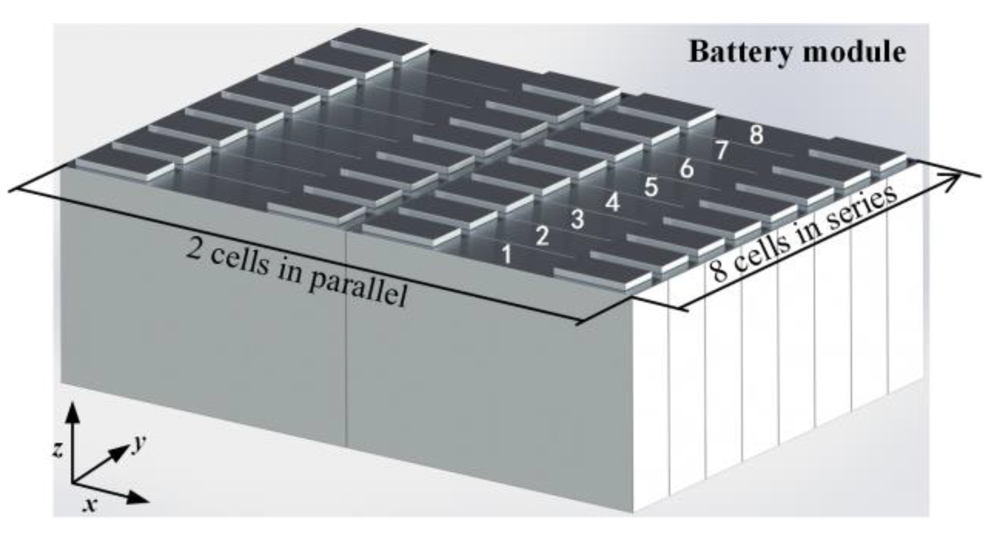
Figure 2.
The layout of liquid cold plates for battery module cooling.

Figure 3.
Schematic diagram of liquid cold plates with serpentine flow paths: (a) 3D model; (b) 2D model of flow paths.
Figure 3.
Schematic diagram of liquid cold plates with serpentine flow paths: (a) 3D model; (b) 2D model of flow paths.
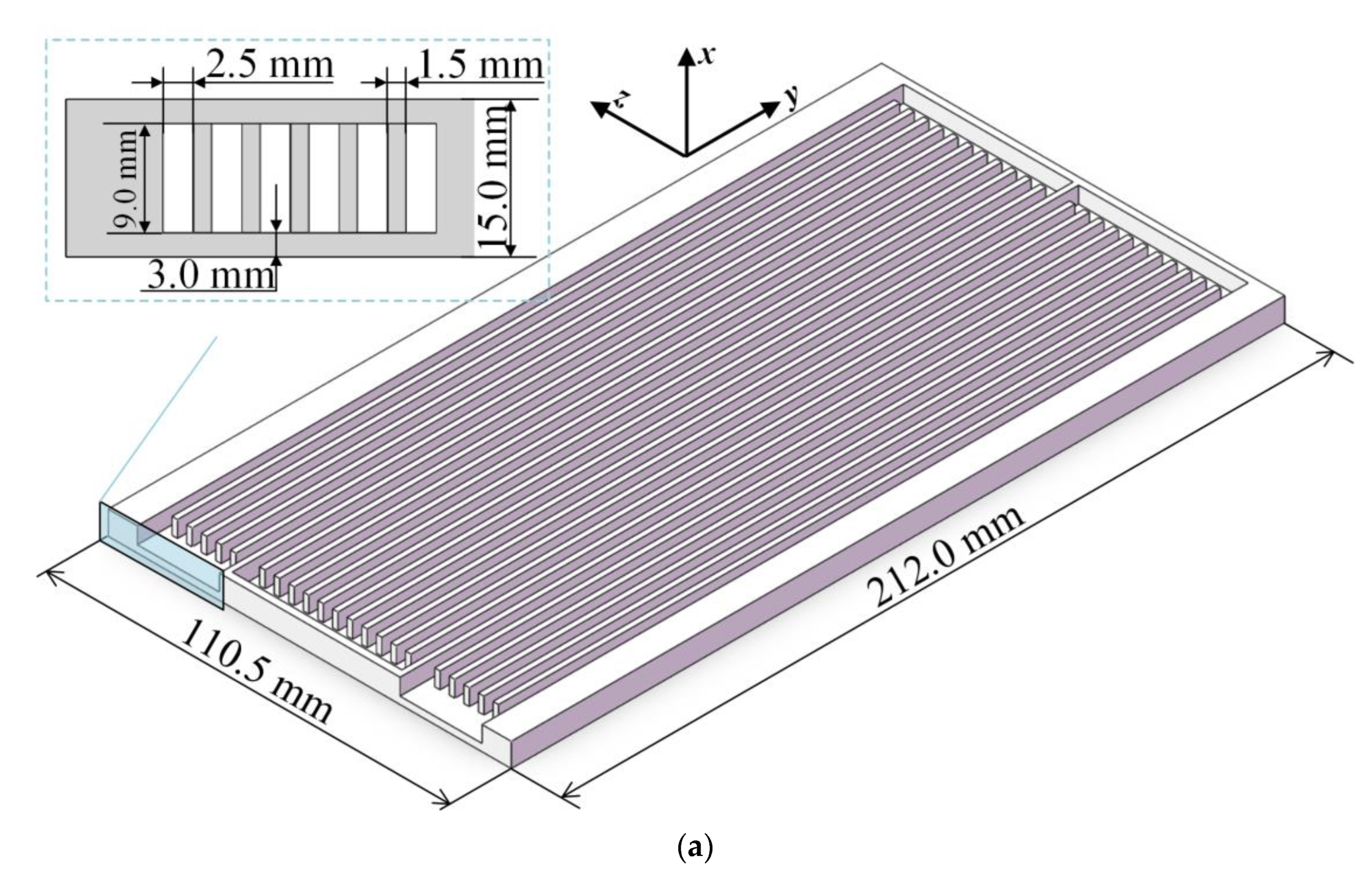

Figure 4.
Schematic of grids for the computational domain: (a) 3D structure; (b) sectional grids at½2 height plane.
Figure 4.
Schematic of grids for the computational domain: (a) 3D structure; (b) sectional grids at½2 height plane.
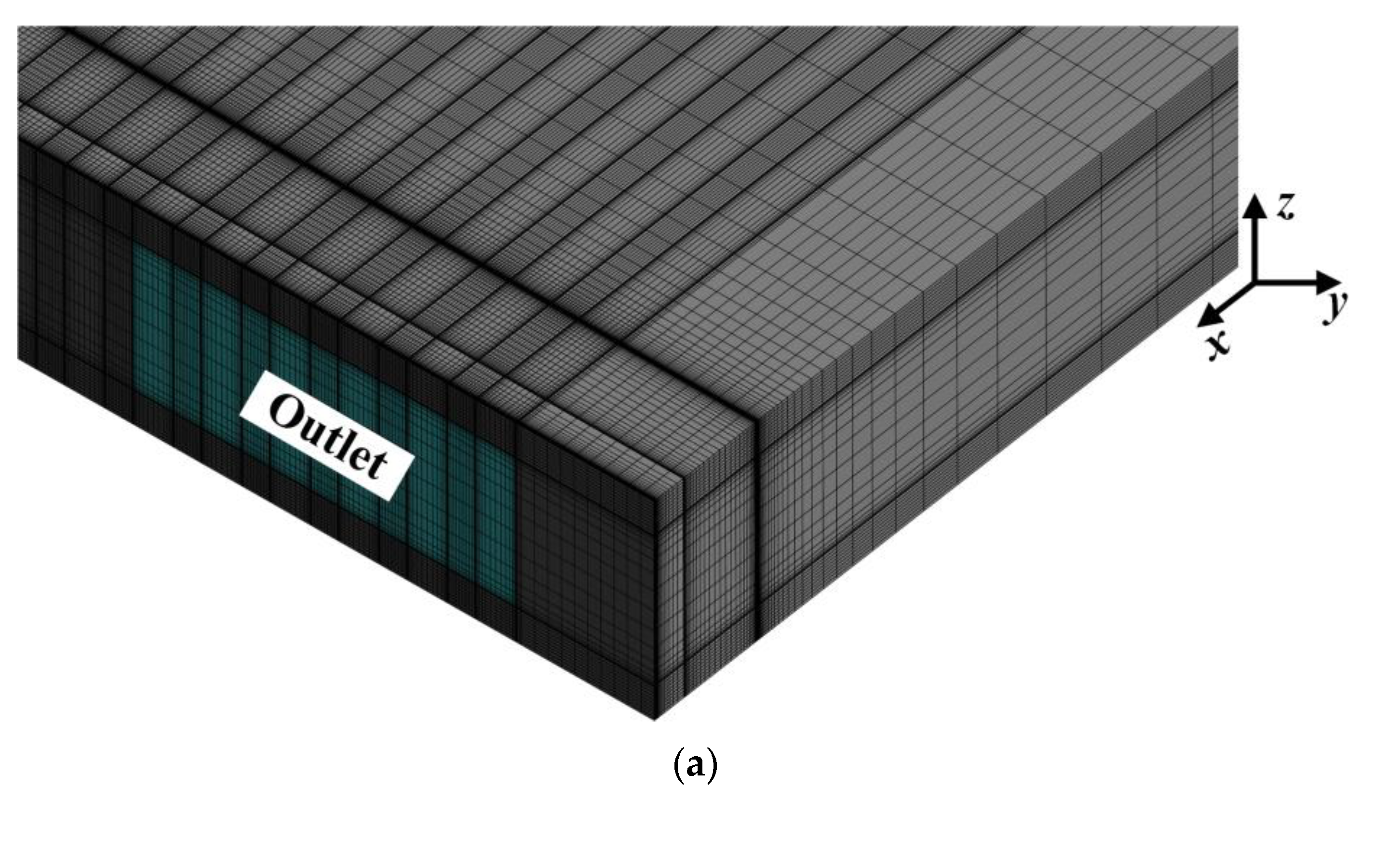
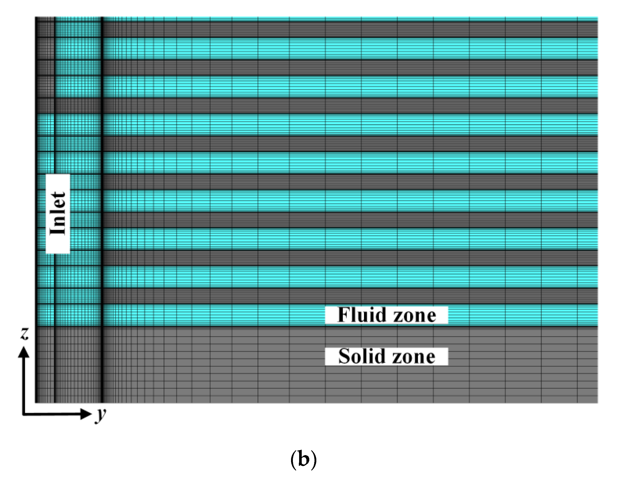
Figure 5.
The effects of grid number on the numerically solved results: (a) Maximum temperature difference; (b) Pressure drop.
Figure 5.
The effects of grid number on the numerically solved results: (a) Maximum temperature difference; (b) Pressure drop.

Figure 6.
The flowchart of the optimization procedure.
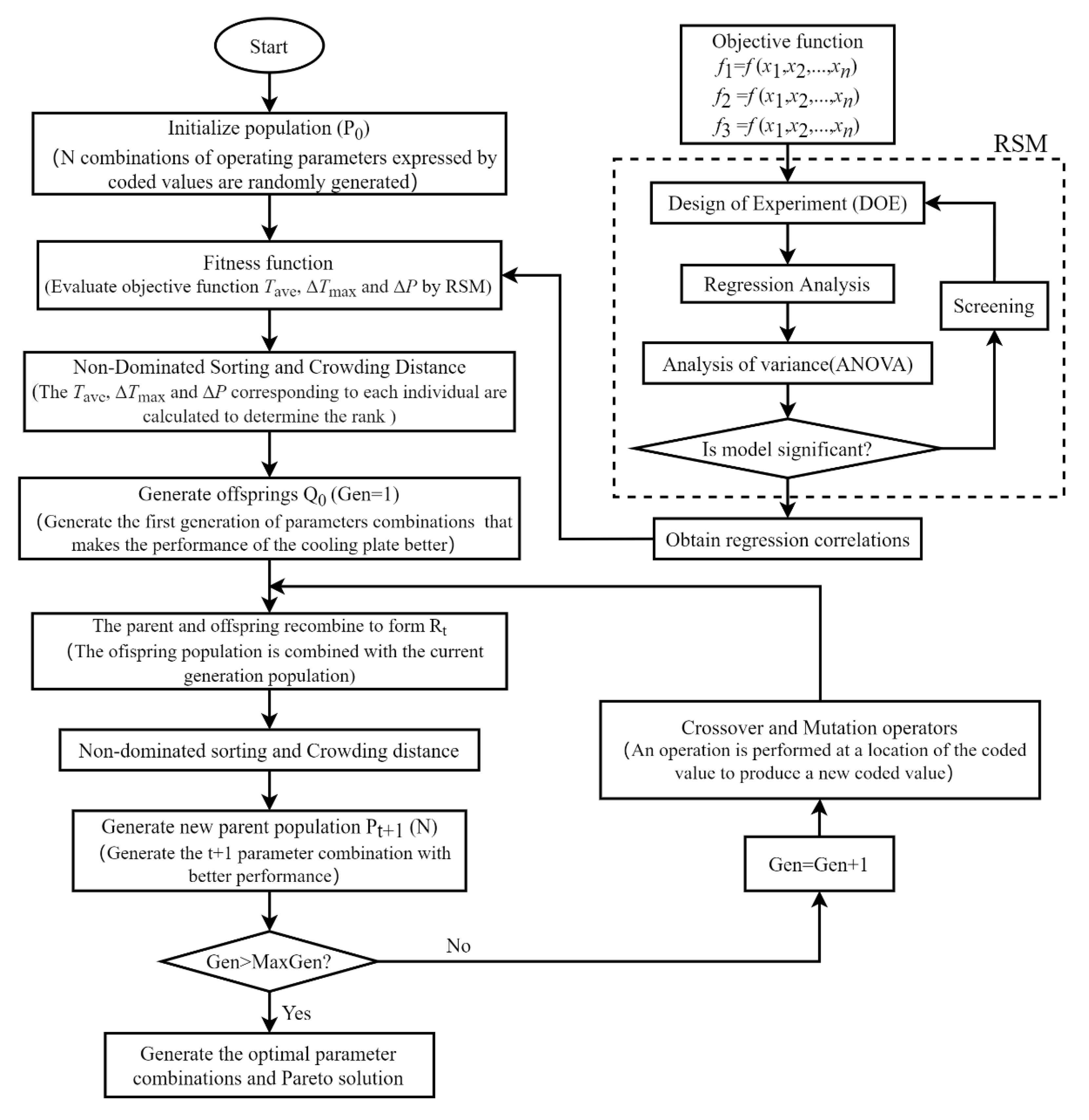
Figure 7.
Temperature distribution of the liquid cold plate under different flow rates when Q = 35 W and Tin = 25 °C: (a) = 0.0019 kg·s−1 (b) = 0.0134 kg·s−1 (c) = 0.0249 kg·s−1.
Figure 7.
Temperature distribution of the liquid cold plate under different flow rates when Q = 35 W and Tin = 25 °C: (a) = 0.0019 kg·s−1 (b) = 0.0134 kg·s−1 (c) = 0.0249 kg·s−1.
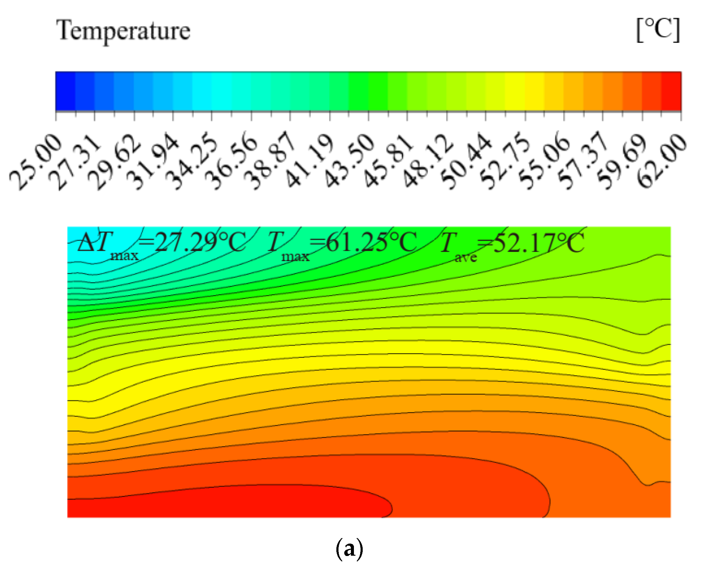

Figure 8.
The variation in pressure drop with mass flow rate.

Figure 9.
Temperature distribution in the liquid cold plate under different inlet temperatures when Q = 35 W and = 0.0134 kg·s−1: (a) Tin = 20 °C (b) Tin = 25 °C (c) Tin = 30 °C.
Figure 9.
Temperature distribution in the liquid cold plate under different inlet temperatures when Q = 35 W and = 0.0134 kg·s−1: (a) Tin = 20 °C (b) Tin = 25 °C (c) Tin = 30 °C.
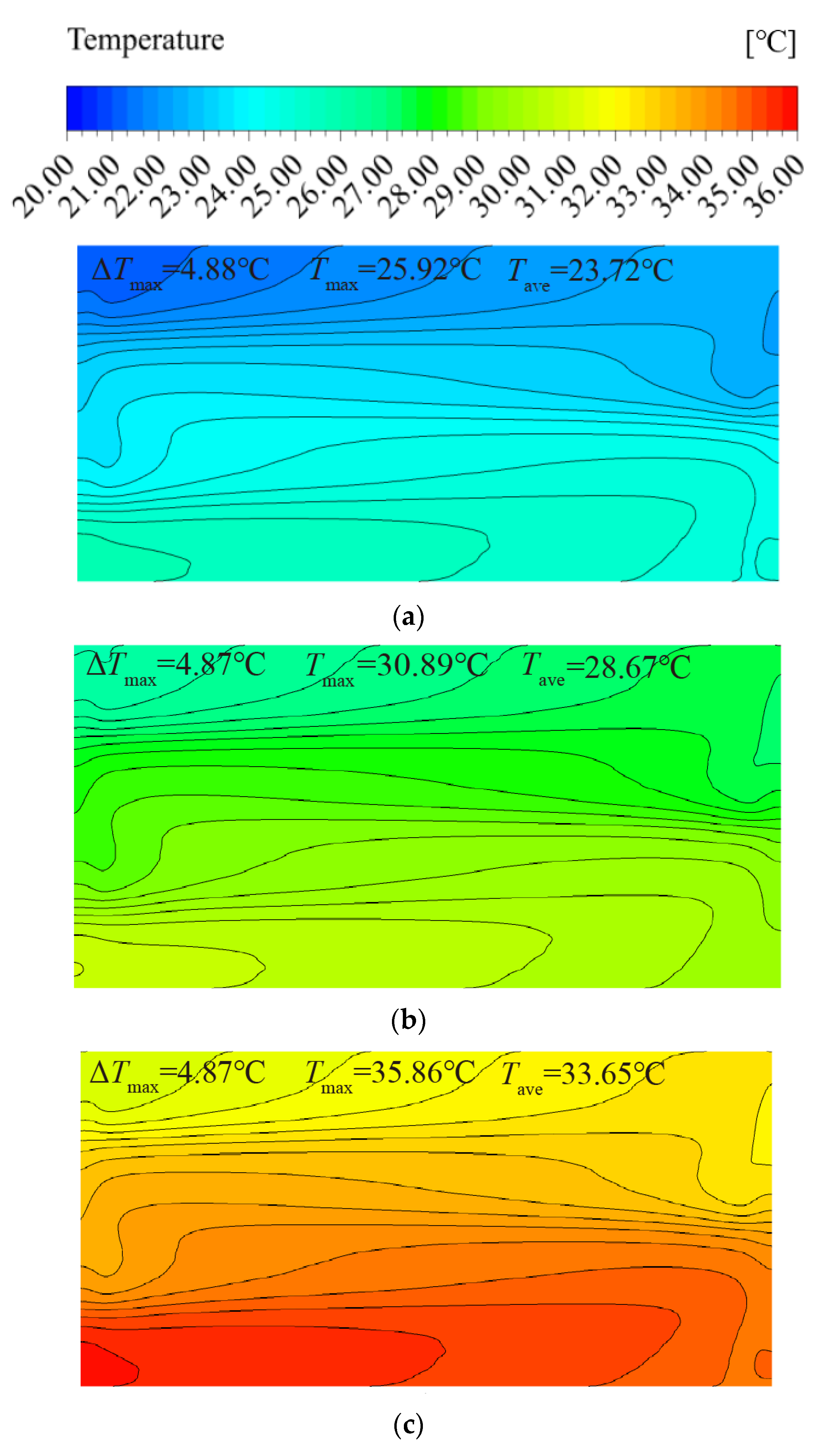
Figure 10.
3D surface plots of the combined effects on the average temperature: (a) Q·
; (b) Tin·
(c) Q·Tin.
Figure 10.
3D surface plots of the combined effects on the average temperature: (a) Q·
; (b) Tin·
(c) Q·Tin.
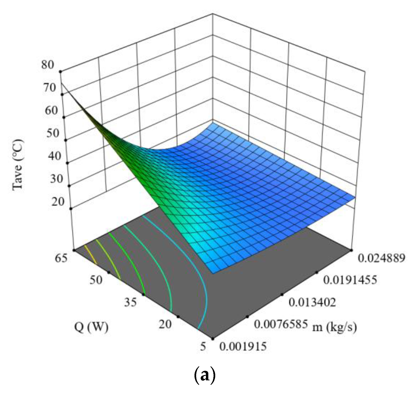
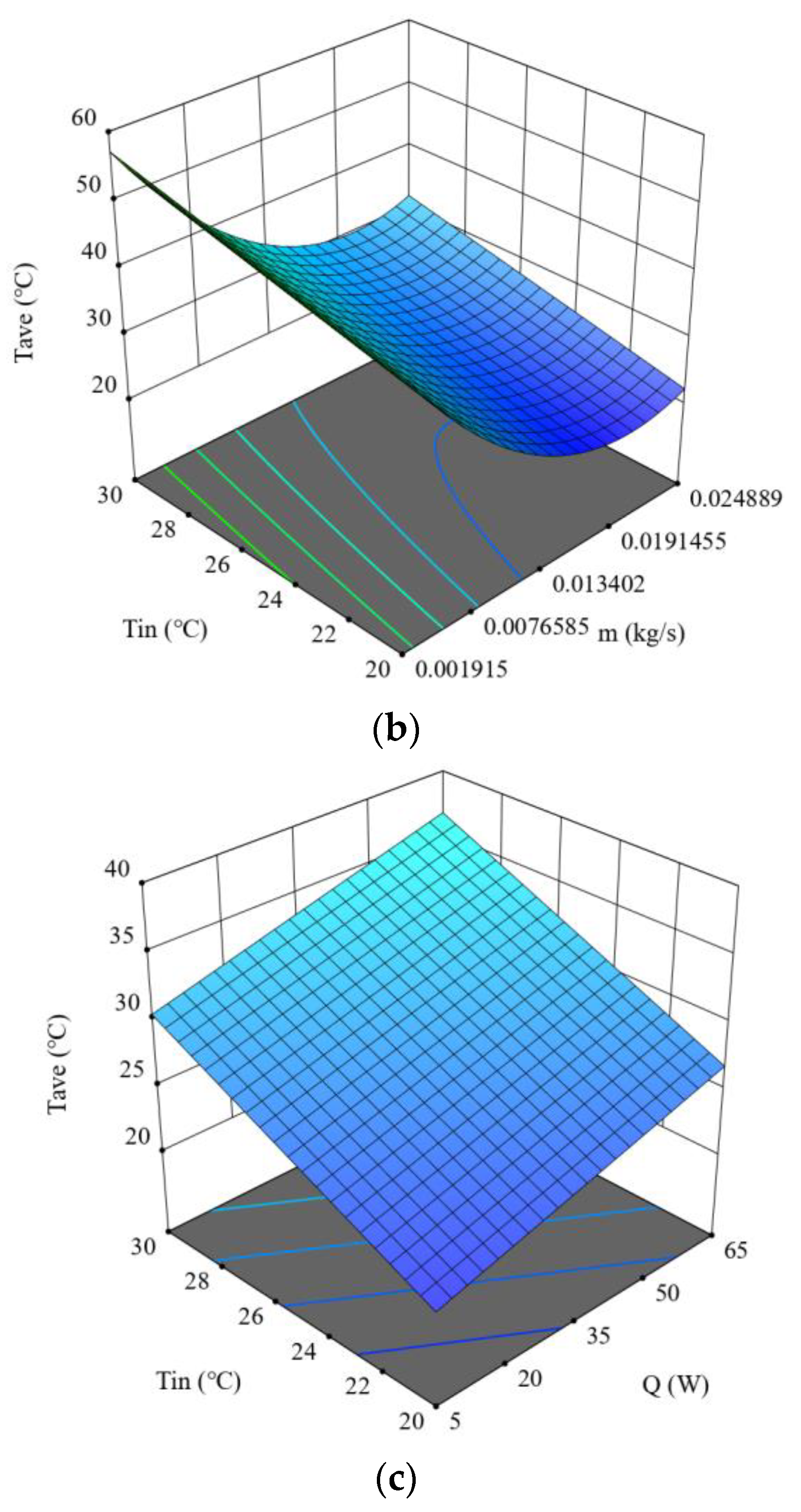
Figure 11.
3D surface plots of the combined effects on the maximum temperature difference: (a) Q·; (b) Tin· (c) Q·Tin.
Figure 11.
3D surface plots of the combined effects on the maximum temperature difference: (a) Q·; (b) Tin· (c) Q·Tin.
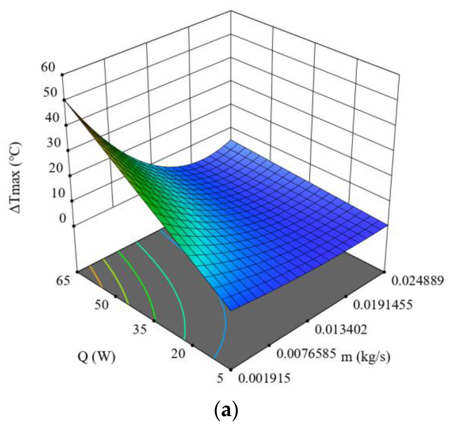

Figure 12.
3D surface plot of the combined effects of inlet temperature and flow rate on the pressure drop.
Figure 12.
3D surface plot of the combined effects of inlet temperature and flow rate on the pressure drop.
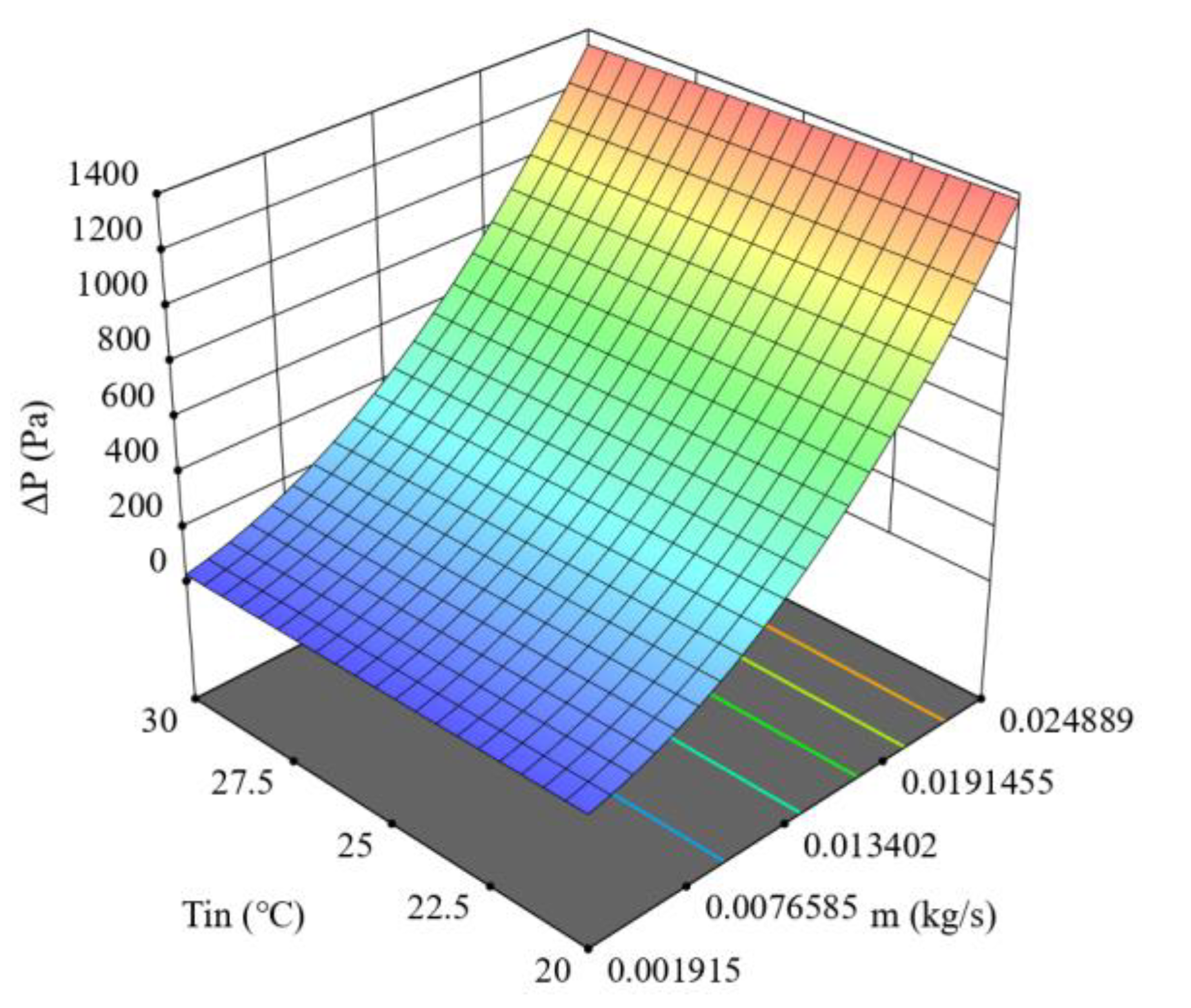
Figure 13.
The Pareto solutions for average temperature and pressure drop under different discharging rates: (a) 1.0 C (b) 2.0 C (c) 3.0 C (d) 4.0 C.
Figure 13.
The Pareto solutions for average temperature and pressure drop under different discharging rates: (a) 1.0 C (b) 2.0 C (c) 3.0 C (d) 4.0 C.
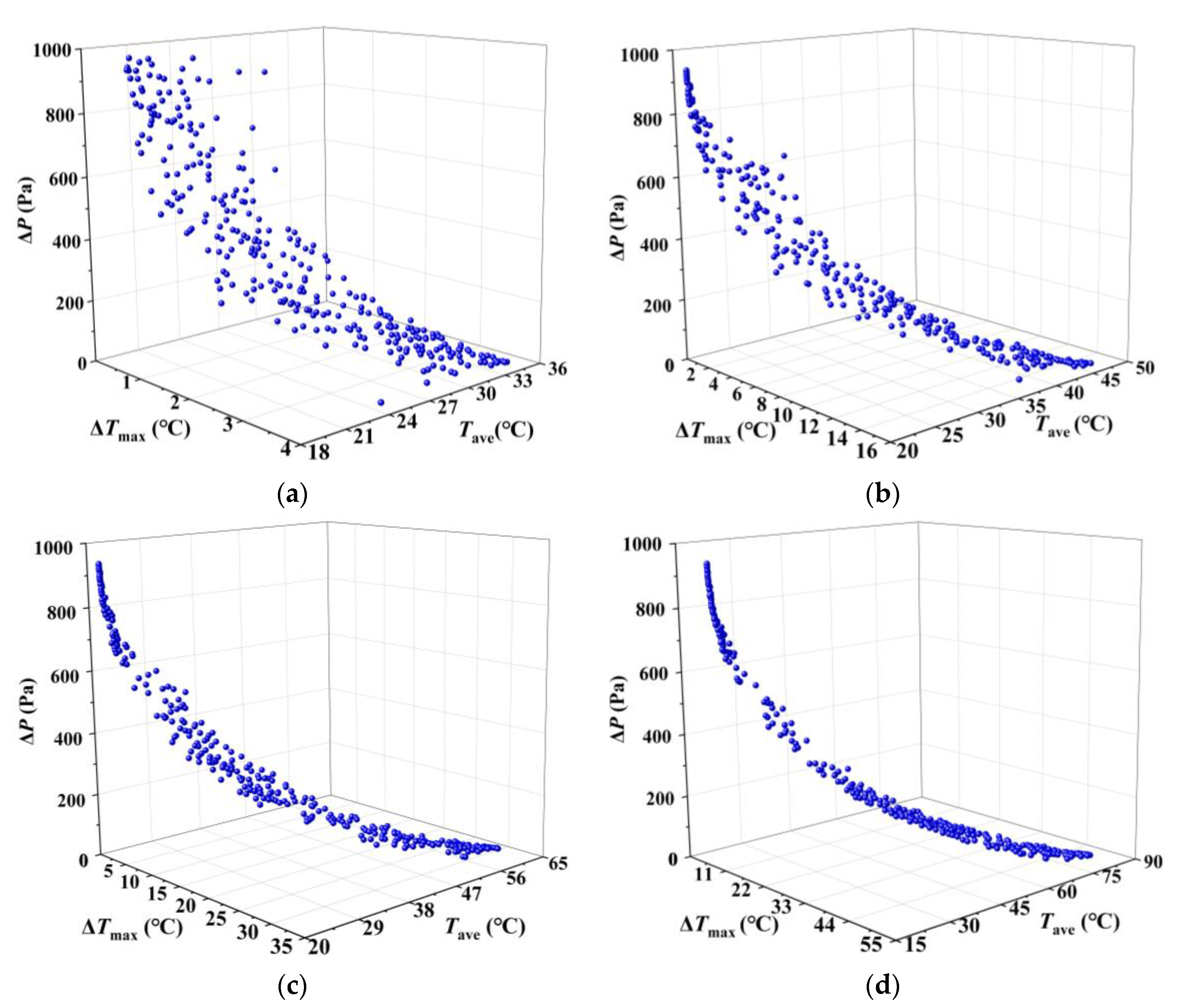
Table 1.
Design variables and levels of the condition.
| S/No. | Design Variables | Level | ||
|---|---|---|---|---|
| −1 | 0 | 1 | ||
| 1 | Flow rate, kg·s−1 | 0.0019 | 0.0134 | 0.0249 |
| 2 | Average heat generation rate, W | 5 | 35 | 65 |
| 3 | Inlet temperature, °C | 20 | 25 | 30 |
Table 2.
Simulation design and corresponding results.
| Variables (Code) | Variables (Actual Value) | Response | |||||||
|---|---|---|---|---|---|---|---|---|---|
| No. | Q | Tin | , kg·s−1 | Q, W | Tin, °C | Tave, °C | ΔTmax, °C | ΔP, Pa | |
| case1 | −1 | −1 | −1 | 0.0019 | 5 | 20 | 23.89 | 3.89 | 30.45 |
| case2 | 1 | −1 | −1 | 0.0249 | 5 | 20 | 20.31 | 0.38 | 1377.06 |
| case3 | −1 | 1 | −1 | 0.0019 | 65 | 20 | 70.53 | 50.52 | 30.45 |
| case4 | 1 | 1 | −1 | 0.0249 | 65 | 20 | 23.98 | 4.95 | 1377.06 |
| case5 | −1 | −1 | 1 | 0.0019 | 5 | 30 | 33.83 | 3.86 | 25.09 |
| case6 | 1 | −1 | 1 | 0.0249 | 5 | 30 | 30.3 | 0.38 | 1344.95 |
| case7 | −1 | 1 | 1 | 0.0019 | 65 | 30 | 80.46 | 50.88 | 25.09 |
| case8 | 1 | 1 | 1 | 0.0249 | 65 | 30 | 33.93 | 4.98 | 1344.93 |
| case9 | −1 | 0 | 0 | 0.0019 | 35 | 25 | 52.17 | 27.29 | 27.77 |
| case10 | 1 | 0 | 0 | 0.0249 | 35 | 25 | 27.13 | 2.67 | 1360.47 |
| case11 | 0 | −1 | 0 | 0.0134 | 5 | 25 | 25.52 | 0.69 | 448.10 |
| case12 | 0 | 1 | 0 | 0.0134 | 65 | 25 | 31.83 | 9.05 | 448.10 |
| case13 | 0 | 0 | −1 | 0.0134 | 35 | 20 | 23.72 | 4.88 | 461.87 |
| case14 | 0 | 0 | 1 | 0.0134 | 35 | 30 | 33.65 | 4.87 | 434.67 |
| case15 | 0 | 0 | 0 | 0.0134 | 35 | 25 | 28.67 | 4.87 | 448.10 |
Table 3.
GAMULTIOBJ function parameters.
| Parameters | Values |
|---|---|
| PopulationSize | 1000 |
| ParetoFraction | 0.3 |
| MaxGenerations | 200 |
| MaxStallGenerations | 200 |
| FunctionTolerance | 10−10 |
| Number of variables | 2 |
Table 4.
The ANOVA for the average temperature (before elimination).
| Source | Sum of Squares | Degrees of Freedom | Mean Square | F-Value | p-Value |
|---|---|---|---|---|---|
| Model | 4626.93 | 12 | 385.58 | 3.452 × 10⁹ | <0.0001 |
| 1568.31 | 1 | 1568.31 | 1.404 × 10¹⁰ | <0.0001 | |
| Q | 19.87 | 1 | 19.87 | 1.779 × 10⁸ | <0.0001 |
| Tin | 49.51 | 1 | 49.51 | 4.433 × 10⁸ | <0.0001 |
| · Q | 923.81 | 1 | 923.81 | 8.271 × 10⁹ | <0.0001 |
| · Tin | 0.0006 | 1 | 0.0006 | 5484.01 | <0.0001 |
| Q·Tin | 0.0002 | 1 | 0.0002 | 1790.70 | <0.0001 |
| · | 331.45 | 1 | 331.45 | 2.968 × 10⁹ | <0.0001 |
| Q·Q | 5.682 × 10⁻⁷ | 1 | 5.682 × 10⁻⁷ | 5.09 | 0.0587 |
| Tin·Tin | 5.682 × 10⁻⁹ | 1 | 5.682 × 10⁻⁹ | 0.0509 | 0.8280 |
| · Q·Tin | 0.0002 | 1 | 0.0002 | 1450.47 | <0.0001 |
| 2· Q | 141.99 | 1 | 141.99 | 1.271 × 10⁹ | <0.0001 |
| 2·Tin | 8.100 × 10⁻⁶ | 1 | 8.100 × 10⁻⁶ | 72.52 | <0.0001 |
| · Q·Q | 1.000 × 10⁻⁷ | 1 | 1.000 × 10⁻⁷ | 0.8800 | 0.3844 |
| Residual | 7.818 × 10⁻⁷ | 8 | 1.117 × 10⁻⁷ | ||
| Lack of fit | 7.818 × 10⁻⁷ | 3 | 3.909 × 10⁻⁷ | ||
| Pure error | 0.0000 | 5 | 0.0000 | ||
| Cor total | 4626.93 | 19 |
Table 5.
The ANOVA for the maximum temperature difference (before elimination).
| Source | Sum of Squares | Degrees of Freedom | Mean Square | F-Value | p-Value |
|---|---|---|---|---|---|
| Model | 4273.94 | 13 | 328.76 | 5.904 × 10⁹ | <0.0001 |
| 302.85 | 1 | 302.85 | 5.439 × 10⁹ | <0.0001 | |
| Q | 34.94 | 1 | 34.94 | 6.276 × 10⁸ | <0.0001 |
| Tin | 0.0000 | 1 | 0.0000 | 323.27 | <0.0001 |
| · Q | 892.30 | 1 | 892.30 | 1.602 × 10¹⁰ | <0.0001 |
| ·Tin | 0.0122 | 1 | 0.0122 | 2.199 × 10⁵ | <0.0001 |
| Q·Tin | 0.0215 | 1 | 0.0215 | 3.866 × 10⁵ | <0.0001 |
| · | 280.85 | 1 | 280.85 | 5.044 × 10⁹ | <0.0001 |
| Q·Q | 2.784 × 10⁻⁷ | 1 | 2.784 × 10⁻⁷ | 5.00 | 0.0667 |
| Tin·Tin | 2.784 × 10⁻⁷ | 1 | 2.784 × 10⁻⁷ | 5.00 | 0.0667 |
| ·Q·Tin | 0.0174 | 1 | 0.0174 | 3.123 × 10⁵ | <0.0001 |
| 2·Q | 120.35 | 1 | 120.35 | 2.161 × 10⁹ | <0.0001 |
| 2·Tin | 0.0038 | 1 | 0.0038 | 68,640.45 | <0.0001 |
| ·Q·Q | 6.250 × 10⁻⁷ | 1 | 6.250 × 10⁻⁷ | 11.22 | 0.0154 |
| Residual | 3.341 × 10⁻⁷ | 6 | 5.568 × 10⁻⁸ | ||
| Lack of fit | 3.341 × 10⁻⁷ | 1 | 3.341 × 10⁻⁷ | ||
| Pure error | 0.0000 | 5 | 0.0000 | ||
| Cor total | 4273.94 | 19 |
Table 6.
The ANOVA for the pressure drop (before elimination).
| Source | Sum of Squares | Degrees of Freedom | Mean Square | F-Value | p-Value |
|---|---|---|---|---|---|
| Model | 4.748 × 10⁶ | 9 | 5.275 × 10⁵ | 1.833 × 10⁵ | <0.0001 |
| 4.443 × 10⁶ | 1 | 4.443 × 10⁶ | 1.544 × 10⁶ | <0.0001 | |
| Q | 0.0001 | 1 | 0.0001 | 0.0000 | 0.9955 |
| Tin | 1043.63 | 1 | 1043.63 | 362.74 | <0.0001 |
| ·Q | 0.0001 | 1 | 0.0001 | 0.0000 | 0.9950 |
| ·Tin | 357.98 | 1 | 357.98 | 124.43 | <0.0001 |
| · | 1.665 × 10⁵ | 1 | 1.665 × 10⁵ | 57,870.36 | <0.0001 |
| Q·Q | 0.0028 | 1 | 0.0028 | 0.0010 | 0.9756 |
| Tin·Tin | 0.1196 | 1 | 0.1196 | 0.0416 | 0.8425 |
| Residual | 28.77 | 10 | 2.88 | ||
| Lack of fit | 28.77 | 5 | 5.75 | ||
| Pure error | 0.0000 | 5 | 0.0000 | ||
| Cor total | 4.748 × 10⁶ | 19 |
Table 7.
Accuracy verification of Pareto optimal solution.
| Discharging Rate | Q kg·s−1 | Tin °C | Predicted/CFD Results of Tave, °C | Predicted/CFD Results of ΔTmax, °C | Predicted/ CFD Results of ΔP, Pa | Error of Tave % | Error of ΔTmax % | Error of ΔP % |
|---|---|---|---|---|---|---|---|---|
| 1.0 C | 0.0156 | 26.86 | 27.09/ 27.31 | 0.51/0.58 | 579.82/ 582.91 | −0.81 | −12.07 | −0.53 |
| 0.0057 | 28.29 | 30.68/ 29.68 | 2.46/2.49 | 108.95/ 105.79 | 3.37 | −1.20 | 2.99 | |
| 2.0 C | 0.0163 | 25.33 | 26.03/ 27.07 | 2.14/2.32 | 629.69/ 628.76 | −3.84 | −7.88 | 0.15 |
| 0.0118 | 28.00 | 31.18/ 29.85 | 3.36/3.12 | 356.27/ 356.58 | 4.46 | 7.63 | −0.09 | |
| 3.0 C | 0.0174 | 21.13 | 21.9/ 24.44 | 3.86/4.37 | 718.26/ 722.97 | −10.39 | −11.67 | −0.65 |
| 0.0158 | 25.54 | 27.34/ 29.14 | 4.05/4.79 | 593.37/ 593.15 | −6.18 | −15.50 | 0.04 | |
| 4.0 C | 0.0199 | 20.00 | 24.08/ 24.72 | 3.58/3.97 | 919.68/ 920.81 | −2.59 | −9.82 | −0.12 |
| 0.0203 | 20.23 | 23.60/ 23.25 | 3.42/3.87 | 743.05/ 743.85 | 1.51 | −11.63 | −0.11 |
Table 8.
The variation range of objectives based on Pareto optimal solution.
| Discharging Rate | ΔTmax, °C | Tave, °C | ΔP, Pa |
|---|---|---|---|
| 1.0 C | 0.29~3.90 | 20.03~33.82 | 24.39~966.91 |
| 2.0 C | 1.11~15.66 | 20.07~45.40 | 24.44~941.94 |
| 3.0 C | 2.17~31.39 | 20.14~60.72 | 24.56~940.21 |
| 4.0 C | 3.43~50.92 | 20.22~80.22 | 24.53~936.84 |
Publisher’s Note: MDPI stays neutral with regard to jurisdictional claims in published maps and institutional affiliations. |
© 2022 by the authors. Licensee MDPI, Basel, Switzerland. This article is an open access article distributed under the terms and conditions of the Creative Commons Attribution (CC BY) license (https://creativecommons.org/licenses/by/4.0/).
Share and Cite
MDPI and ACS Style
Wei, L.; Zou, Y.; Cao, F.; Ma, Z.; Lu, Z.; Jin, L. An Optimization Study on the Operating Parameters of Liquid Cold Plate for Battery Thermal Management of Electric Vehicles. Energies 2022, 15, 9180. https://doi.org/10.3390/en15239180
AMA Style
Wei L, Zou Y, Cao F, Ma Z, Lu Z, Jin L. An Optimization Study on the Operating Parameters of Liquid Cold Plate for Battery Thermal Management of Electric Vehicles. Energies. 2022; 15(23):9180. https://doi.org/10.3390/en15239180
Chicago/Turabian StyleWei, Lichuan, Yanhui Zou, Feng Cao, Zhendi Ma, Zhao Lu, and Liwen Jin. 2022. "An Optimization Study on the Operating Parameters of Liquid Cold Plate for Battery Thermal Management of Electric Vehicles" Energies 15, no. 23: 9180. https://doi.org/10.3390/en15239180
Note that from the first issue of 2016, this journal uses article numbers instead of page numbers. See further details here.