
Modal Analysis of Tubing Considering the Effect of Fluid–Structure Interaction

1
College of Petroleum Engineering, Southwest Petroleum University, Chengdu 610500, China
2
CNPC Key Laboratory of Oil & Gas Storage and Transportation, Southwest Petroleum University, Chengdu 610500, China
3
CCDC Downhole Service Company, CNPC, Chengdu 610500, China
*
Author to whom correspondence should be addressed.
Energies 2022, 15(2), 670; https://doi.org/10.3390/en15020670
Submission received: 17 November 2021
/
Revised: 12 January 2022
/
Accepted: 14 January 2022
/
Published: 17 January 2022
(This article belongs to the Collection State of the Art Geo-Energy Technology in China)
Abstract
:When tubing is in a high-temperature and high-pressure environment, it will be affected by the impact of non-constant fluid and other dynamic loads, which will easily cause the tubing to vibrate or even resonate, affecting the integrity of the wellbore and safe production. In the structural modal analysis of the tubing, the coupling effect of the fluid and the tubing needs to be considered at the same time. In this paper, a single tubing is taken as an example to simulate and analyze the modal changes of the tubing under dry mode and wet mode respectively, and the effects of fluid solid coupling effect, inlet pressure, and ambient temperature on the modal of the tubing are discussed. After considering the fluid–structure interaction effect, the natural frequency of tubing decreases, but the displacement is slightly larger. The greater the pressure in the tubing, the greater the equivalent stress on the tubing body, so the natural frequency is lower. Furthermore, after considering the fluid–solid coupling effect, the pressure in the tubing is the true pulsating pressure of the fluid. The prestress applied to the tubing wall changes with time, and the pressures at different parts are different. At this time, the tubing is changed at different frequencies. Vibration is prone to occur, that is, the natural frequency is smaller than the dry mode. The higher the temperature, the lower the rigidity of the tubing and the faster the strength attenuation, so the natural frequency is lower, and tubing is more prone to vibration. Both the stress intensity and the elastic strain increase with the increase of temperature, so the displacement of the tubing also increases.
1. Introduction
With the continuous development of high-temperature, high-pressure, and high-yield gas wells, the difficulty of natural gas exploitation is increasing, which puts forward higher requirements for wellbore integrity [1,2]. Tubing is an important part of natural gas development. It is in a special environment and the load is complex and changeable [3,4]. The tubing will be affected by the impact of unsteady fluid and other dynamic loads, which easily cause vibration and even resonance of the tubing string [5,6]. This will not only affect the mechanical properties of the tubing, but accelerate the fatigue failure and affect the integrity of the wellbore and safe production [7].
Many domestic and foreign scholars have conducted research on the modal analysis of pipes or tubing strings. Lenwoue [8] established a poro-elasto-plastic model using nonlinear finite element software, which aimed at analyzing the influence of drill string vibration cyclic loads on the development of the wellbore natural fracture. Xu [9] established an FEM of tubing erosion based on erosion mode, fluid–solid coupling, and the impact of sand. The erosion rule and failure region on the tubing were obtained. Zhang [10] studied the dynamical modeling, multipulse orbits, and chaotic dynamics of cantilevered pipe conveying pulsating fluid with harmonic external force using the energy-phase method. Jiang [11] analyzed the modal characteristics of the simplified U-shaped tubing structure under fluid–structure interaction using ANSYS Workbench software. Wróbel [12] undertook experimental investigations in order to identify the influence of hydraulic pressure on the natural frequencies and mode shapes of a basic hydraulic line model. Xin [13] analyzed the two typical tubings (straight pipe and curved pipe) using the finite element method (FEM) in ADINA software, in order to solve the problem whereby the vibration of a hydraulic pipe poses a severe safety concern in aircraft. Lubecki [14] presented experimental studies of dynamic changes in the length of a microhydraulic hose under the influence of step pressure and flow load. Chai [15] proposed a simplified bilinear stiffness and damping model according to hysteresis loops of the clamp obtained from experimental testing. Then, the finite element model of an L-type tubing system with clamps was established using Timoshenko beam theory in combination with the aforementioned stiffness-damping model. Sekacheva [16] proposed a method for determining the probability of the occurrence of increased vibrations using modal analysis in the ANSYS Workbench software package. Wu [17] used the multiple scale method to obtain an equivalent nonlinear wave equation from the complicated nonlinear governing equation describing the fluid conveyed in a pipe. Guo [18] has established a nonlinear flow-induced vibration model of tubing string by using the micro-element method and energy method with the Hamiltonian variational principle, in order to address the vibration failure problem of the tubing string induced by high-speed fluid flow in the tubing of HPHT oil and gas well. Nan [19] comprehensively analysed the dynamic failure modes and safety criteria of buried tubings based on the study of the dynamic response characteristics of tubings.
However, when analyzing the mechanical properties of the tubing, it is not rigorous to only conduct dry modal analysis and consider less the influence of the fluid–structure interaction effect on the modal characteristics of the tubing. It is necessary to consider the characteristics of fluid and tubing and the interaction between them at the same time, which not only effectively saves the analysis time and cost, but also ensures that the simulation results are closer to the laws of physical phenomena [20,21]. However, it also increases the complexity of tubing mechanics analysis [22].
Based on the mathematical principles of fluid mechanics, solid mechanics, and vibration mechanics, the modal changes of the tubing under dry mode and wet mode are simulated and analyzed by using the finite element method, and the effects of fluid–structure interaction, inlet pressure, and temperature in the tubing on the calculation results are discussed.
2. Vibration Mechanics Model of Tubing
Structural mode mostly refers to the mode in vacuum without considering the influence of a surrounding fluid. This mode is called “dry mode” [23]. There is fluid in the tubing, and some tubings are even placed in the fluid, so that their inner and outer walls are surrounded by the fluid. The complex changes of fluid density and pressure have a great impact on the tubing mode, which cannot be ignored. This inherent mode taking into account the influence of surrounding fluid is called “wet mode”.
The fluid–structure interaction should be considered in the stress analysis of the tubing. The coupling mode adopted is bidirectional fluid–structure interaction [24,25], that is, the data exchange is mutual. Both the fluid analysis results are transmitted to the solid structure, and the solid analysis results (such as displacement, velocity and acceleration) are transmitted back to the fluid. The tubing and the fluid are discussed separately. The vibration equation of the tubing is:
where [Mt], [Ct], and [Kt] are the mass matrix, damping matrix, and stiffness matrix of tubing; is the excitation of fluid to the tubing; is the external excitation of the tubing; is the displacement column vector of the tubing, is the velocity column vector of the tubing; is the acceleration column vector of the tubing.
The wave equation of the fluid is [26]:
where [Mf], [Cf], and [Kf] are the mass matrix, damping matrix, and stiffness matrix of the fluid; is the excitation of the tubing to the fluid; is the pressure column vector of fluid, and and are the first-order derivative column vector and the second-order derivative column vector of fluid pressure with respect to time, respectively.
The excitation of fluid to tubing and the excitation of tubing to fluid can be expressed as follows:
where ρf is the fluid density and [Itp] is the inertia matrix of the tubing cross section.
The simultaneous Equations (1)–(4) can be used:
Standardize Equation (5):
where [M], [C], and [K] are the mass coupling matrix, damping coupling matrix, and stiffness coupling matrix of tubing and fluid, respectively; is the parameter column vector, while and are the first-order derivative column vector and the second-order derivative column vector of parameter with respect to time, respectively.
The wet modal analysis of the tubing can be carried out by combining Equations (6)–(10).
If the influence of damping and external excitation of the tubing is ignored, i.e., [Ct] = 0, = 0, the simultaneous Equations (1)–(4) can be used:
Standardize Equation (5):
The wet modal analysis ignoring the influence of damping and external excitation of the tubing can be carried out by combining Equations (7), (9), (10), and (12).
3. Dry Mode Finite Element Analysis of Tubing
3.1. Establishment of Finite Element Mechanical Mode
As gas storage wells often face extreme conditions of “large injection and large production” and “strong injection and strong production”, it is more convincing to use tubing calculations for gas storage wells. It is difficult to establish the full-scale model of the tubing due to the length. Therefore, a single tubing with a length of 9.6 m is taken as an example to establish the finite element model. The outer diameter is 177.8 mm (some gas storage wells have larger tubing sizes), the wall thickness is 10.36 mm, the elastic modulus of the tubing is 206 GPa, the Poisson’s ratio is 0.3, and the density is 7850 kg/m3. The tubing model is discretized with eight node hexahedron elements. The number of nodes is 167,060 and the number of elements is 24,966. The tubing mesh is shown in Figure 1. Taking any hexahedral element on the tubing as an example, its dimensions are dx, dy, and dz. The normal stress is σx, σy, σz, and the shear stress is τxy, τyz, τzx. The corresponding three-dimensional stress diagram is shown in Figure 2.
The external load of the tubing mainly includes the pressure of the fluid, the gravity of the tubing, and temperature. Before the wet mode simulation, the vibration mode of the tubing in vacuum should be determined, and the influence of fluid flow on the tubing mode, i.e., dry mode analysis, should not be considered temporarily. Because at least one end of the tubing is fixed, the constrained mode of the tubing is simulated directly.
3.2. Simulation
ANSYS workbench finite element software was used to solve the modal analysis of the tubing.
After the finite element mechanics model is established, constraints and loads are applied to it in the “Mechanical” module of the workbench solver. The constraint conditions for the tubing are generally divided into no constraint, one end constraint and both ends constraint. Since the solver cannot solve unconstrained conditions, two settings of one end constraint and both ends of the tubing are set, and the constraint mode is fixed. When performing load sensitivity analysis, it is also necessary to apply initial pressure and temperature loads.
Set the initial conditions of the modal analysis in the “Modal” module. The default maximum number of modes for the solver is 6. These modes are the rigid body modes that each object has, that is, the translational modes in 3 directions and the rotational modes in 3 directions, so the maximum number of modes needs to be increased (only the first 6 modes are considered for tubing modal analysis) [27] to find the corresponding modal at more frequencies. Here, the maximum number of modes is increased to 20. Then, it can be solved.
3.3. Dry Modal Analysis of Tubing
Under the boundary conditions of constraining only one end and both ends of the tubing, the modal analysis is carried out. The simulation results of the natural frequencies of each order of the oil tubing in both cases are shown in Figure 3. It can be seen from the figure that after constraining both ends of the tubing, the natural frequency of the tubing body is higher than when only one end is constrained. The reason for this is that after the two ends of the tubing are fixed, the stiffness of the tubing increases, that is, the excitation that promotes the resonance of the tubing increases, and the tubing is not prone to vibration.
The number of modes depends on the node degrees of freedom, which should be distinguished from the model. It is the element node rather than the overall model. After the element is divided, each node corresponds to a degree of freedom. The tubing model has 167,060 nodes, but it is not necessary to solve all modes, which is also impractical. The low-frequency modal amplitude is the largest and most dangerous, the high-frequency modal amplitude is very small, and the modal research with high frequency is meaningless. Therefore, only the first few modes at low frequencies need to be studied.
As shown in Figure 4 and Figure 5, when only one end of the tubing is constrained, the seventh mode of the tubing is the first-order Y-direction bending mode. That is, it swings back and forth along the radial Y direction of the tubing, and the vibration frequency is 59.556 Hz at this time. There are three bends in the tubing. The maximum deformation occurs at the unconstrained end of the tubing, and the value is 3.152 mm. Similarly, at this frequency, the eighth mode of the tubing is the first-order X-direction bending mode. That is, it swings back and forth along the radial X direction of the tubing. The bending part and the maximum deformation part are similar to the seventh mode.
When the two ends of the tubing are constrained, the fifth mode is the first-order Y-direction bending mode, and the vibration frequency is 60.592 Hz. Different from the tubing that only constrains one end, although the tubing also has three bends, the large deformation appears in the three bends. Moreover, due to the action of gravity, the maximum deformation occurs at the lowest bending point (in the direction of gravity acceleration) of the three bends, and the value is about 2.355 mm. At this vibration frequency, the sixth mode of the tubing is the first-order X-direction bending mode, and the bending part and maximum deformation part are similar to the fifth mode.
It can be seen from the above results that when only one end of the tubing is constrained, the other end is in a free state, and the deformation of the whole tubing will be transmitted to the free end. Therefore, for the tubing fixed at the wellhead, an important reason for installing packer near the bottom of the well is to prevent the bottom of the tubing from swinging greatly under the excitation of a specific frequency. However, large deformation will appear in the middle of the tubing after both ends are restrained, which easily causes buckling of the tubing [28]. Therefore, some effective measures need to be taken to deal with such problems, such as thickening the tubing wall thickness, placing centralizers [29], adding titanium alloy tubing or expansion joints, etc.
As shown in Figure 6, the ninth mode of the tubing is the first-order torsional mode when only one end is constrained. That is, the tubing rotates back and forth around its own axis, and the vibration frequency is 81.48 Hz. The maximum deformation of the tubing occurs at the bottom section and the value is 2.335 mm. The 11th mode of the tubing is the first-order torsional mode when the two ends are constrained, and the vibration frequency is 162.98 Hz. The maximum deformation of the tubing occurs in the middle, and the value is basically the same as the displacement of the tubing when only one end is constrained. In this case, the overall displacement of the tubing is symmetrically distributed from the middle to both ends.
As shown in Figure 7 and Figure 8, the second-order and third-order X-direction bending modes of the tubing under two constraints are shown. It can be seen that the arch bending number of the tubing increases with the increase of the order, but the vibration mode and large deformation position of the tubing are similar to the first-order. It can also be found that the maximum displacement of the tubing under the two constraints of the second-order X-direction bending modes is 3.127 mm and 2.354 mm, respectively, and the maximum displacement of the tubing under the two constraints of the third-order X-direction bending modes is 3.109 mm and 2.354 mm, respectively. Compared with the first-order displacement, it can be seen that the amplitude of the low-frequency mode is large and the amplitude of the high-frequency mode is small, which verifies the previous conclusion.
4. Wet Modal Finite Element Analysis of Tubing
The influence of fluid flow should be considered in the wet modal analysis of tubing, so the fluid area needs to be established separately in the calculation. Considering the fluid–structure interaction effect, the modal analysis results of the tubing will be more accurate. When the pressure load in the tubing is applied, the imported pressure data are the real flow data of the fluid. Similarly, the influence of deformation on fluid flow in the tubing can also be studied inversely through the calculated tubing deformation data, that is, the bidirectional fluid–structure interaction effect. The established finite element model of the tubing and the fluid in the tubing are shown in Figure 9 (a is the tubing model and b is the fluid model).
The eight-node hexahedron element is used to mesh the tubing and the fluid model in the tubing. The mesh model is shown in Figure 10. The external wall of all tubing is defined as boundary wall, the surface on the fluid side of the fluid–structure interface is defined as boundary interfacef, and the surface on the tubing side of the fluid–structure interface is defined as boundary interfaces. The two surfaces form a fluid–structure interaction interface to realize the data transfer between the tubing and the fluid in the tubing. This is also the reason why the model is divided by a hexahedral eight node element. If tetrahedral mesh is used, the calculation results may not converge, resulting in inaccurate modal analysis.
The calculation process is divided into two steps. Firstly, the fluid flow in the tubing should be simulated, that is, after the boundary conditions of inlet and outlet of the tubing are determined, the pressure and temperature distribution in the tubing under steady-state conditions should be calculated. Secondly, these load data need to be applied to the inner wall of the tubing, as shown in Figure 11. At this time, the load in the tubing is no longer a two-dimensional constant load or a uniformly varying linear load, but a load formed by the real flow of fluid acting on the inner wall of the tubing. The temperature and pressure values of each element divided by the tubing are different, which is difficult to obtained by the analytical method.
5. Analysis of Influencing Factors of Tubing Mode
5.1. Influence of Fluid–Structure Interaction Effect on Tubing Mode
Assuming that the tubing is constrained at both ends, the wet modal analysis of the tubing is carried out, as shown in Figure 12a. It can be seen from the figure that the natural frequency of the tubing considering the fluid–structure interaction effect is small. The reason for this is that after considering the fluid–structure interaction effect, the research object includes not only the tubing, but also the high-temperature and high-pressure natural gas flowing in the tubing. The overall mass increases obviously, so the natural frequency decreases.
As can be seen from Figure 12b, with the increase of order, the difference of tubing natural frequency gradually increases, but the difference proportion gradually decreases. This shows that in the process of increasing the order, the deformation parts of the tubing increase, and the influence of fluid–structure interaction on the vibration frequency of the tubing decreases gradually. However, in the actual gas production process, high-order frequency rarely occurs. For the frequency within the 14th order, the influence of fluid–structure interaction effect on tubing mode cannot be ignored.
Figure 13 shows the maximum displacement of the tubing under two modal analysis methods. It can be seen from Figure 13 that the maximum displacement of the tubing is large when the natural frequency is small, so the maximum displacement of the tubing in wet mode is slightly larger. The first and second-order modes of the tubing are single, and there is only one large deformation part. All deformations are concentrated in the center of the tubing since both ends are constrained, and the displacement decreases gradually along both ends of the tubing. For the third-order modes and above, the large deformation parts gradually increase and will not be concentrated in one place, so the maximum displacement decreases significantly. The 11th order mode of the tubing is the first-order torsional mode. At this time, the tubing rotates back and forth around its own axis. The transverse deformation is not obvious as other orders, and the main deformation part is in the middle of the tubing. The 14th order mode of the tubing is tensile mode. The tensile displacement of the tubing at low frequency is not large, and the end of the tubing is fixed, so the maximum displacement is much smaller than other orders. The frequencies within the 11th and 14th orders are small deformation modes, which show the characteristics of similar frequency and small displacement. In the actual production process, in the case of inevitable resonance, if it can be induced to reach the corresponding torsional or tensile mode, the buckling and deformation damage of the tubing can be reduced as much as possible.
5.2. Influence of Inlet Pressure on Tubing Mode
The tubing is a three-dimensional cylindrical space and the pressure of flow acting on each point of the inner wall is inconsistent, so the inlet pressure of the tubing is taken as the boundary condition. Both ends of the tubing are constrained, and the tubing modes under the two analysis methods are simulated and calculated. The natural frequencies of the tubing are obtained when the inlet pressure is 10 MPa, 20 MPa, 30 MPa, 40 MPa, 50 MPa, and 60 MPa respectively. The influence of temperature is not considered for the time being. The natural frequencies of the tubing under different inlet pressures of the first 14 orders are extracted, as shown in Table 1 and Table 2. The difference curve of tubing natural frequency affected by the fluid–structure interaction effect under different inlet pressure is drawn, as shown in Figure 14.
According to the data in Table 1 and Table 2, the natural frequency of the tubing calculated after considering the fluid–structure interaction effect is small under the same inlet pressure. As shown in Figure 14, in the low-order mode, the difference of tubing natural frequency increases with the gradual increase of inlet pressure. With the increase of order, the difference of tubing natural frequency under different pressures gradually tends to be consistent, indicating that the influence of inlet pressure on tubing natural frequency decreases with the increase of order. When the tubing is in torsional and tensile modes, the natural frequency of the tubing basically does not change.
Figure 15 shows the maximum displacement of the tubing under different inlet pressures. It can be seen that the maximum displacement of tubing corresponding to each order also increases with the gradual increase of inlet pressure. The 11th order is torsional mode and the tubing is twisted along its own axis. The displacement is small, which is independent of the value of inlet pressure. If the fluid–structure interaction effect is not considered, the overall mass of the research object will be reduced, and the maximum displacement of the tubing will be small.
5.3. Effect of Temperature on Tubing Mode
Both ends of the tubing are constrained, and the natural frequencies of the tubing are obtained when the ambient temperature is 30 °C, 40 °C, 50 °C, 60 °C, 70 °C, 80 °C, and 90 °C, respectively. The influence of pressure is not considered for the time being. The natural frequencies of the tubing under different ambient temperatures of the first 14 orders are extracted, as shown in Table 3. The difference curve of tubing natural frequency under different inlet pressure is drawn, as shown in Figure 16.
According to the data in Table 3, the influence trend of temperature on the natural frequency of tubing is similar to that of inlet pressure. The higher the temperature, the smaller the natural frequency of the tubing, which easily causes vibration [30]. With the increase of ambient temperature, the maximum displacement of tubing corresponding to each order increases. The large deformation parts of the tubing corresponding to the first and second orders are concentrated, so the maximum displacement is significantly greater than the following orders. In the 3rd to 14th orders, the maximum displacement of the tubing corresponding to 5th and 6th orders is significantly higher than that of other orders. The vibration modes of these two orders of tubing are first-order bending and there are few overall deformation parts, so the displacement of buckling parts is large. After that, the deformation part of the tubing increases with the increase of the order, and the displacement of each buckling part decreases accordingly. The 11th order is torsional mode, and the tubing displacement is small and independent of the value of ambient temperature.
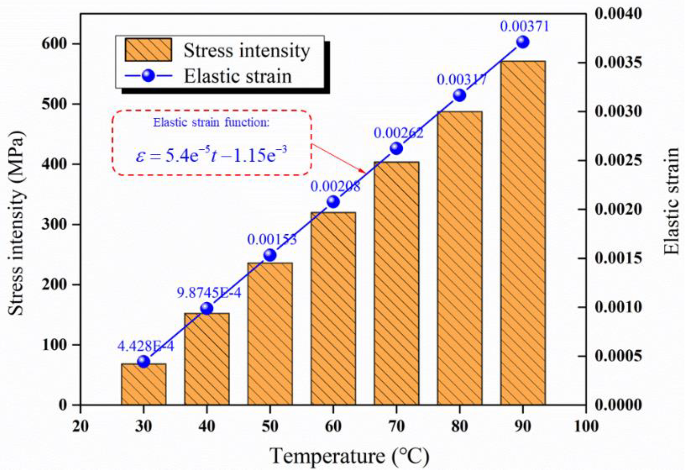
Temperature has a great impact on the strength of the tubing. The stress intensity and strain of the tubing at different temperatures are studied and analyzed, and the results are shown in Figure 17. When the ambient temperature increases from 30 to 90 °C, the stress intensity and elastic strain will increase with the difference of variation law. The increase of elastic strain shows a linear trend. According to the calculated results, the tubing elastic strain function considering the effect of temperature is constructed, and the back calculation error is less than 5%. The increasing trend of stress intensity decreases slowly with the increase of temperature. Therefore, it is inferred that the attenuation rate will gradually accelerate with the continuous increase of temperature.
6. Conclusions
In this paper, the modal changes of tubing under dry mode and wet mode are simulated and compared, and the effects of fluid–structure interaction effect, inlet pressure, and ambient temperature on the tubing modal are discussed. The following conclusions can be drawn:
- After considering the fluid–solid coupling effect, the research objects include tubings and natural gas in the tubing. The mass increases, so the natural frequency decreases, but the displacement is slightly larger. In the actual production process, the buckling and deformation damage of the tubing can be reduced by inducing the corresponding torsional or tensile mode.
- The greater the pressure in the tubing, the greater the equivalent stress on the tubing body, so the tubing is more prone to vibration, i.e., the natural frequency is lower. Furthermore, after considering the fluid–solid coupling effect, the pressure in the tubing is the true pulsating pressure of the fluid. The prestress applied to the tubing wall changes with time, and the pressures at different parts are different. At this time, the tubing is changed at different frequencies. Vibration is prone to occur, i.e., the natural frequency is smaller than the dry mode.
- The higher the temperature, the lower the rigidity of the tubing body and the faster the strength attenuation, so the tubing is more prone to vibration, i.e., the natural frequency is lower. Both the stress intensity and the elastic strain increase with the temperature, so the displacement of the tubing also increases. The influence of temperature on the tubing modal is slightly greater than that of pressure.
Author Contributions
Conceptualization, methodology, software, C.L.; validation, formal analysis, investigation, J.J.; writing—original draft preparation, writing—review and editing, J.D. All authors have read and agreed to the published version of the manuscript.
Funding
This research received no external funding.
Conflicts of Interest
The authors declare no conflict of interest.
References
- Alkhamis, M.; Imqam, A. A Simple Classification of Wellbore Integrity Problems Related to Fluids Migration. Arab. J. Sci. Eng. 2021, 46, 6131–6141. [Google Scholar] [CrossRef]
- Zhang, L.; Yan, X.; Yang, X.; Zhao, X. Evaluation of wellbore integrity for HTHP gas wells under solid-temperature coupling using a new analytical model. J. Nat. Gas Sci. Eng. 2015, 25, 347–358. [Google Scholar] [CrossRef]
- Zhang, Z.; Wang, J.; Li, Y.; Ming, L.; Zhang, C. Effects of instantaneous shut-in of high production gas well on fluid flow in tubing. Pet. Explor. Dev. 2020, 47, 642–650. [Google Scholar] [CrossRef]
- Kou, Z.; Wang, H. Transient Pressure Analysis of a Multiple Fractured Well in a Stress-Sensitive Coal Seam Gas Reservoir. Energies 2020, 13, 3849. [Google Scholar] [CrossRef]
- Jun, L.; Guo, X.; Wang, G.; Liu, Q.; Fang, D.; Huang, L.; Mao, L. Bi-nonlinear vibration model of tubing string in oil & gas well and its experimental verification. Appl. Math. Model. 2020, 81, 50–69. [Google Scholar]
- Liu, J.; Zeng, L.; Guo, X.; Dai, L.; Huang, X.; Cai, L. Nonlinear flow-induced vibration response characteristics of leaching tubing in salt cavern underground gas storage. J. Energy Storage 2021, 41, 102909. [Google Scholar] [CrossRef]
- Zhang, Z.; Wang, J.; Li, Y.; Liu, H.; Meng, W.; Li, L. Research on the influence of production fluctuation of high-production gas well on service security of tubing string. Oil Gas Sci. Technol. Revue d’IFP Energies Nouv. 2021, 76, 54. [Google Scholar] [CrossRef]
- Lenwoue, A.; Deng, J.; Feng, Y.; Li, H.; Oloruntoba, A.; Selabi, N.B.S.; Marembo, M.; Sun, Y. Numerical Investigation of the Influence of the Drill String Vibration Cyclic Loads on the Development of the Wellbore Natural Fracture. Energies 2021, 14, 2015. [Google Scholar] [CrossRef]
- Xu, J.; Mou, Y.; Xue, C.; Ding, L.; Wang, R.; Ma, D. The study on erosion of buckling tubing string in HTHP ultra-deep wells considering fluid–solid coupling. Energy Rep. 2021, 7, 3011–3022. [Google Scholar] [CrossRef]
- Zhang, Y.F.; Yao, M.H.; Zhang, W.; Wen, B.C. Dynamical modeling and multi-pulse chaotic dynamics of cantilevered pipe conveying pulsating fluid in parametric resonance. Aerosp. Sci. Technol. 2017, 68, 441–453. [Google Scholar] [CrossRef]
- Jiang, Y.; Zhu, L. Modal analysis of liquid-filled tubing under fluid-structure interaction by simulation and experiment methods. Vibroeng. Procedia 2018, 21, 42–47. [Google Scholar]
- Wróbel, J.; Blaut, J. Influence of Pressure Inside a Hydraulic Line on Its Natural Frequencies and Mode Shapes. In Proceedings of the International Scientific-Technical Conference on Hydraulic and Pneumatic Drives and Control, Staniszow, Poland, 21–23 October 2020; Springer: Berlin/Heidelberg, Germany, 2020. [Google Scholar]
- Xin, L.; Wang, S.; Ran, L. Modal Analysis of Two Typical Fluid-filled Pipes in Aircraft. In Proceedings of the 2011 International Conference on Fluid Power and Mechatronics, Beijing, China, 17–20 August 2011; pp. 469–473. [Google Scholar]
- Lubecki, M.; Stosiak, M.; Bocian, M.; Urbanowicz, K. Analysis of selected dynamic properties of the composite hydraulic microhose. Eng. Fail. Anal. 2021, 125, 105431. [Google Scholar] [CrossRef]
- Chai, Q.; Zeng, J.; Ma, H.; Li, K.; Han, Q. A dynamic modeling approach for nonlinear vibration analysis of the L-type tubing system with clamps. Chin. J. Aeronaut. 2020, 33, 3253–3265. [Google Scholar] [CrossRef]
- Sekacheva, A.A.; Pastukhova, L.G.; Alekhin, V.N.; Noskov, A.S. Natural frequencies of a vertical tubing element. In Proceedings of the IV International Conference on Safety Problems of Civil Engineering Critical Infrastructures, Ekaterinburg, Russia, 4–5 October 2019; p. 481. [Google Scholar]
- Wu, Q.; Qi, G. Global dynamics of a pipe conveying pulsating fluid in primary parametrical resonance: Analytical and numerical results from the nonlinear wave equation. Phys. Lett. A 2019, 383, 1555–1562. [Google Scholar] [CrossRef]
- Guo, X.; Liu, J.; Wang, G.; Dai, L.; Fang, D.; Huang, L.; He, Y. Nonlinear flow-induced vibration response characteristics of a tubing string in HPHT oil & gas well. Appl. Ocean Res. 2020, 106, 102468. [Google Scholar]
- Jiang, N.; Zhu, B.; Zhou, C.; Li, H.; Wu, B.; Yao, Y.; Wu, T. Blasting vibration effect on the buried tubing: A brief overview. Eng. Fail. Anal. 2021, 129, 105709. [Google Scholar] [CrossRef]
- Tian, X.; Zhou, S.; Hu, L.; Li, W.; He, W. Vibration Fatigue Characteristic of High-Pressure Fuel Pipe Based on Fluid-Solid Coupling Model. J. Vib. Meas. Diagn. 2018, 38, 1234–1239. [Google Scholar]
- Xu, Y.; Zhang, H.; Guan, Z. Dynamic Characteristics of Downhole Bit Load and Analysis of Conversion Efficiency of Drill String Vibration Energy. Energies 2021, 14, 229. [Google Scholar] [CrossRef]
- Luo, J.; Zhang, K.; Liu, J.; Mu, L.; Wang, F. The Study of Tubing Vibration Mechanism in High Pressure Gas Well. World J. Eng. Technol. 2021, 9, 128–137. [Google Scholar] [CrossRef]
- Shi, L.; Zhu, J.; Wang, L.; Chu, S.; Tang, F.P.; Jiang, Y.; Xu, T.; Yu, J. Analysis of Strength and Modal Characteristics of a Full Tubular Pump Impeller Based on Fluid-Structure Interaction. Energies 2021, 14, 6395. [Google Scholar] [CrossRef]
- Zheng, X.; Wang, Z.; Triantafyllou, M.S.; Karniadakis, G.E. Fluid-structure interactions in a flexible pipe conveying two-phase flow. Int. J. Multiph. Flow 2021, 141, 103667. [Google Scholar] [CrossRef]
- Mohmmed, A.O.; Al-Kayiem, H.H.; Osman, A.B.; Sabir, O. One-way coupled fluid-structure interaction of gas-liquid slug flow in a horizontal pipe: Experiments and simulations. J. Fluids Struct. 2020, 97, 103083. [Google Scholar] [CrossRef]
- Huang, Z.; Li, L.; Hu, G. Fatigue Life Prediction of Tubing Strings in Natural Gas Wells; Chongqing University Press: Chongqing, China, 2012. [Google Scholar]
- Lee, G.; Jhung, M.; Bae, J.; Kang, S. Numerical Study on the Cavitation Flow and Its Effect on the Structural Integrity of Multi-Stage Orifice. Energies 2021, 14, 1518. [Google Scholar] [CrossRef]
- Lian, Z.; Mou, Y.; Liu, Y.; Xu, D. Buckling behaviors of tubing strings in HTHP ultra-deep wells. Nat. Gas Ind. 2018, 38, 89–94. [Google Scholar]
- Mou, Y.; Lian, Z.; Zhang, Q.; Lu, Z.; Li, J. Study on influence of centralizer on buckling behavior of tubing string in ultra-deep gas well. J. Saf. Sci. Technol. 2018, 14, 109–114. [Google Scholar]
- Bęben, D. The Influence of Temperature on Degradation of Oil and Gas Tubing Made of L80-1 Steel. Energies 2021, 14, 6855. [Google Scholar] [CrossRef]
Figure 1.
Mesh of single tubing model.

Figure 2.
Three dimensional stress diagram of hexahedral element of tubing.
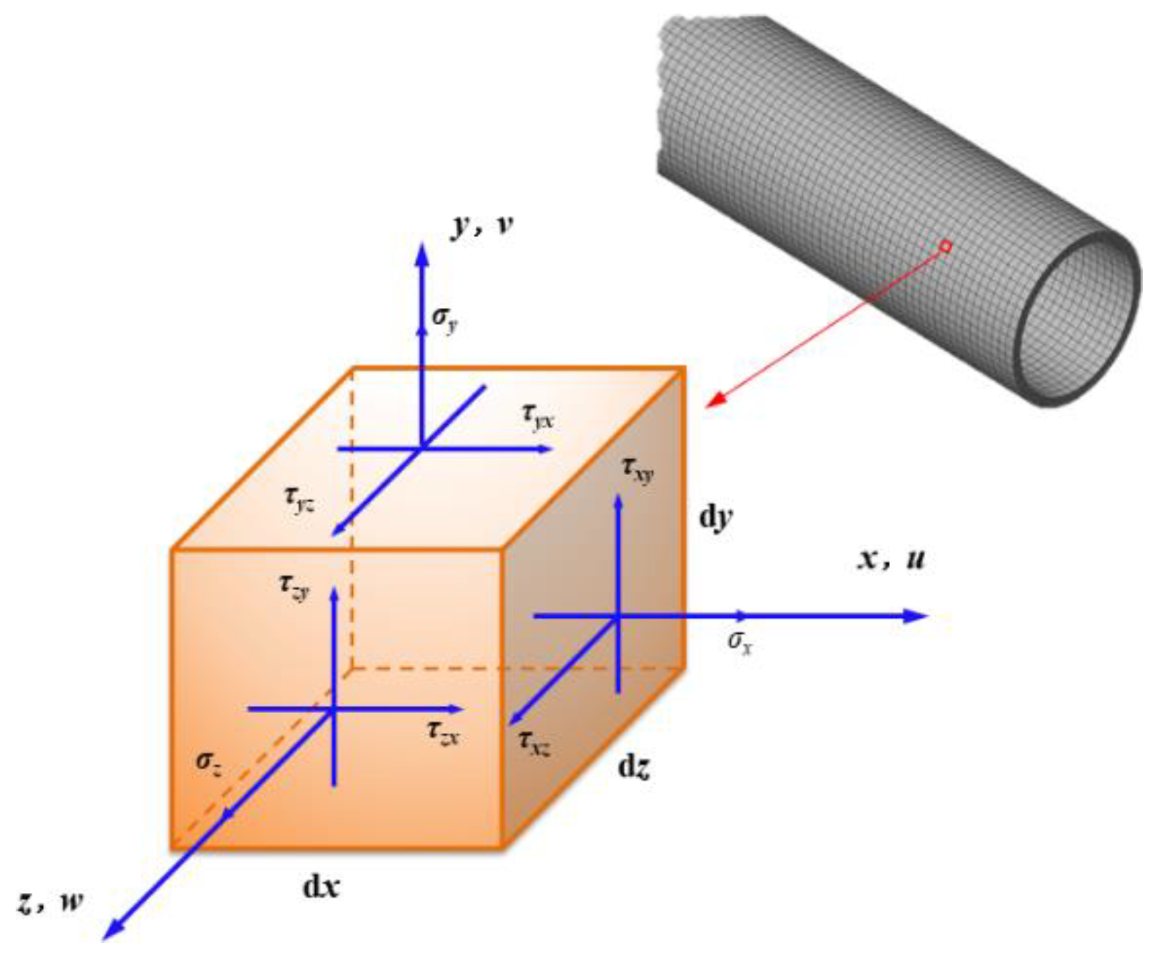
Figure 3.
Comparison of natural frequencies of tubing under two constraints.
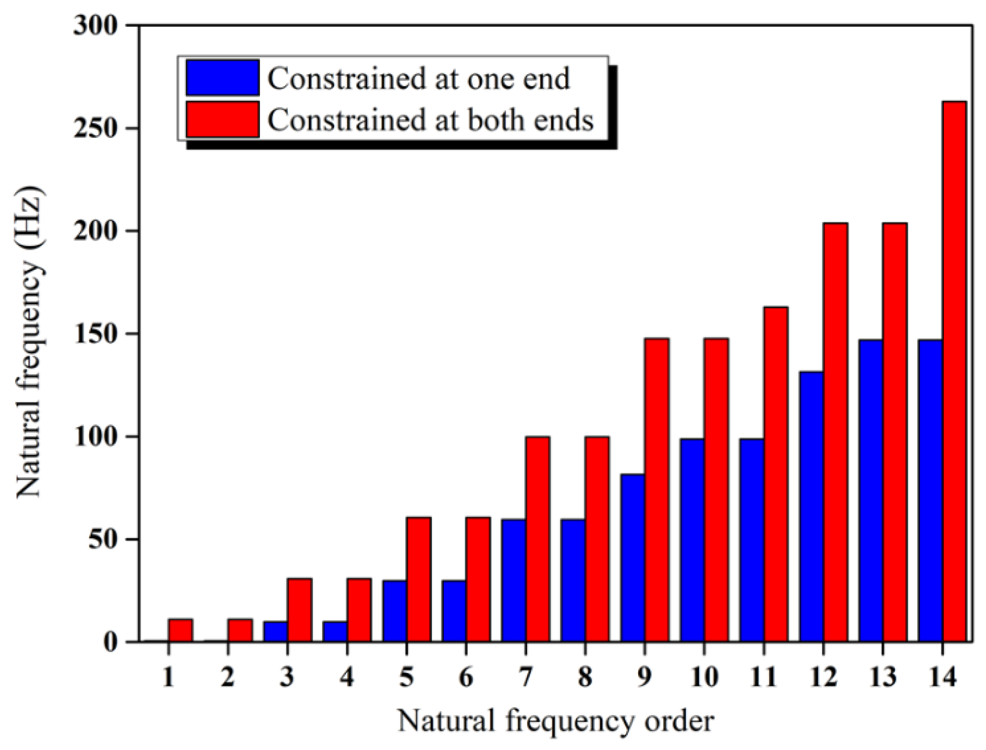
Figure 4.
First-order Y-direction bending state of tubing under two constraints.

Figure 5.
First-order X-direction bending state of tubing under two constraints.
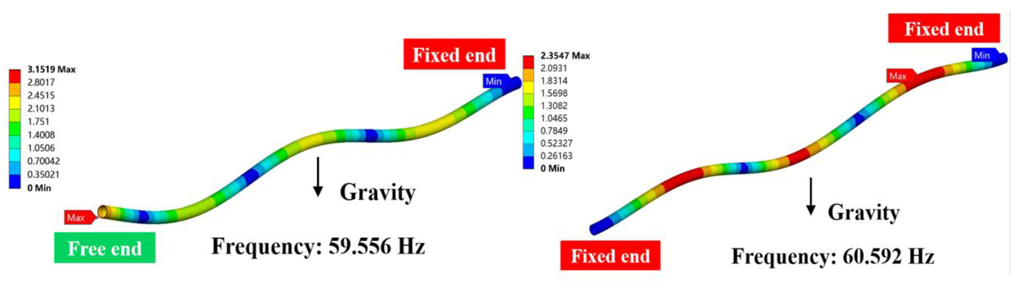
Figure 6.
First-order torsional mode of tubing under two constraints.

Figure 7.
Second-order X-direction bending modes of tubing under two constraints.
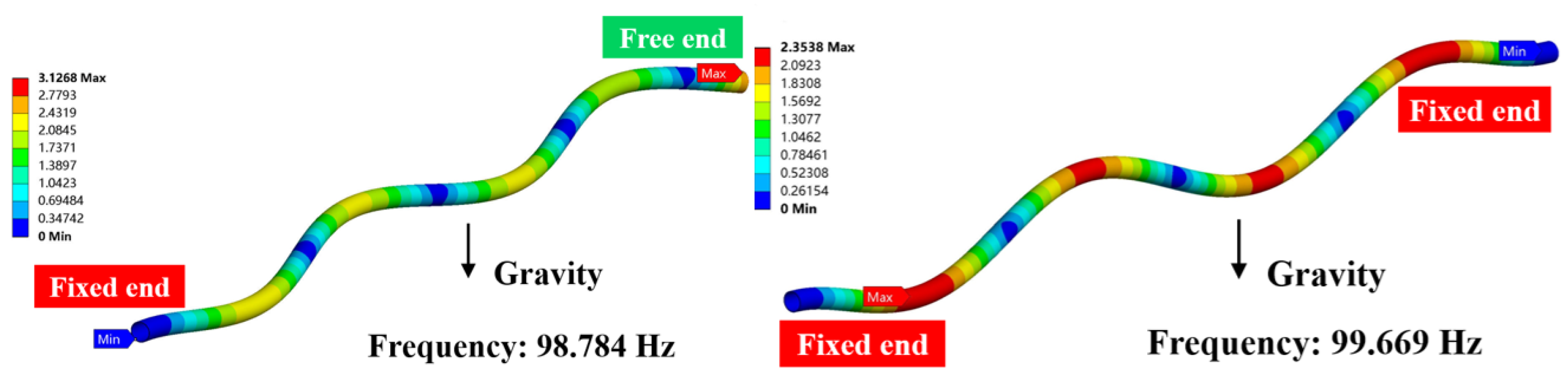
Figure 8.
Third-order X-direction bending modes of tubing under two constraints.

Figure 9.
Finite element model of the tubing and the fluid in the tubing. ((a) is the tubing model and (b) is the fluid model).
Figure 9.
Finite element model of the tubing and the fluid in the tubing. ((a) is the tubing model and (b) is the fluid model).
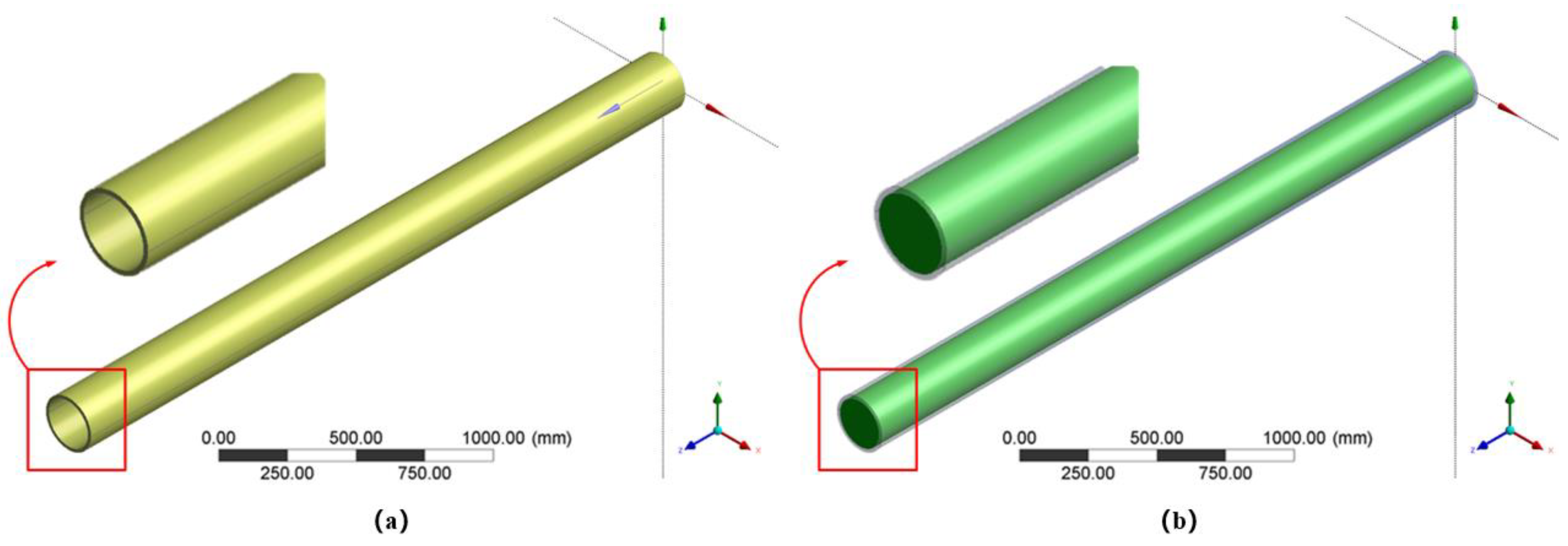
Figure 10.
Mesh generation of the tubing and the fluid in the tubing ((a) is the tubing mesh and (b) is the fluid mesh).
Figure 10.
Mesh generation of the tubing and the fluid in the tubing ((a) is the tubing mesh and (b) is the fluid mesh).

Figure 11.
Pressure load caused by fluid flow in tubing inner wall.
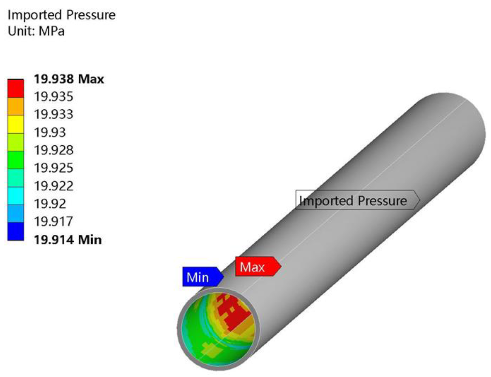
Figure 12.
Natural frequencies of tubing under two modal analysis methods ((a) is natural frequencies of tubing under two modal analysis methods, (b) is difference of natural frequency of tubing under two modal analysis methods).
Figure 12.
Natural frequencies of tubing under two modal analysis methods ((a) is natural frequencies of tubing under two modal analysis methods, (b) is difference of natural frequency of tubing under two modal analysis methods).
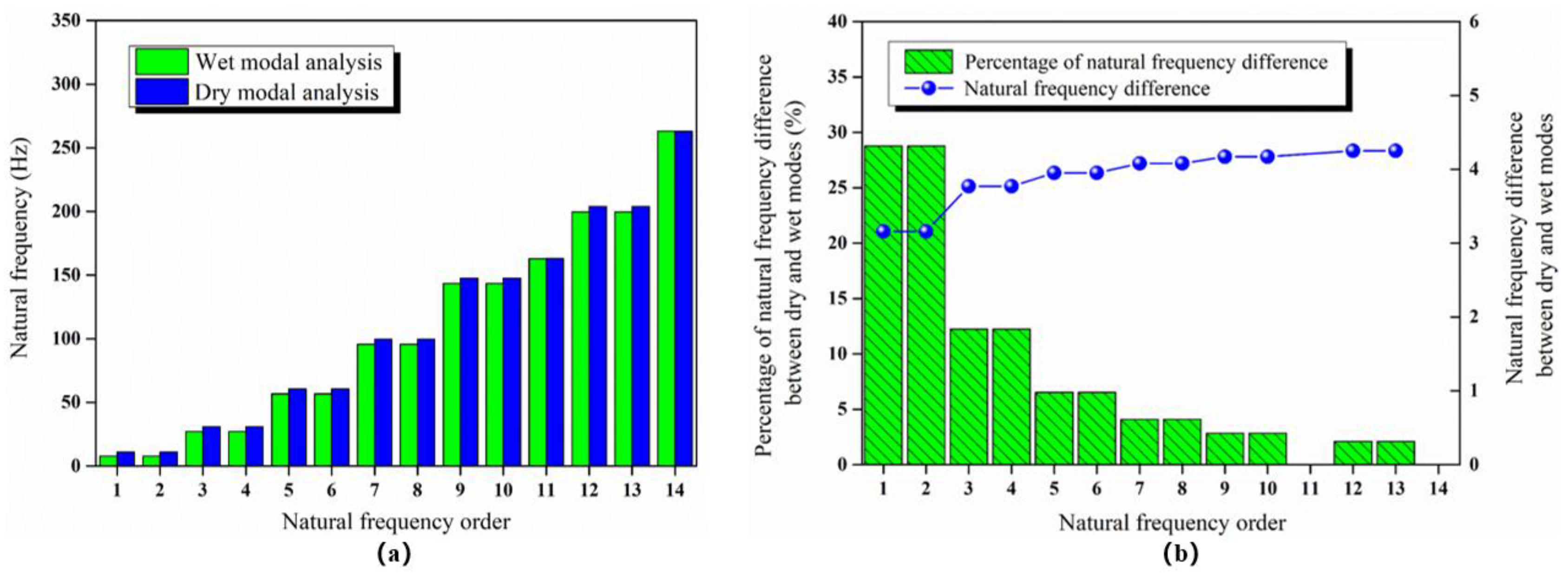
Figure 13.
Maximum displacement of tubing under two modal analysis methods.
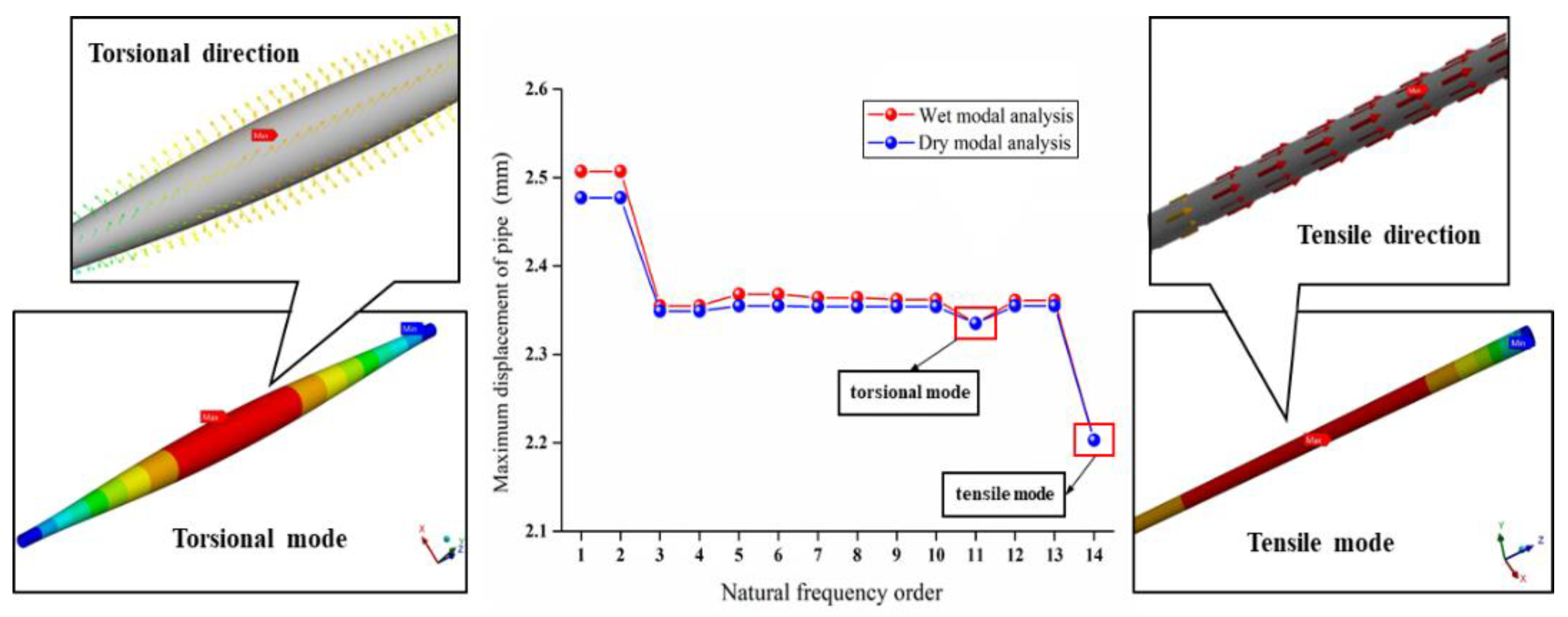
Figure 14.
Influence of fluid-structure interaction effect on natural frequency of tubing under different inlet pressure.
Figure 14.
Influence of fluid-structure interaction effect on natural frequency of tubing under different inlet pressure.

Figure 15.
Maximum displacement of tubing under different inlet pressure.
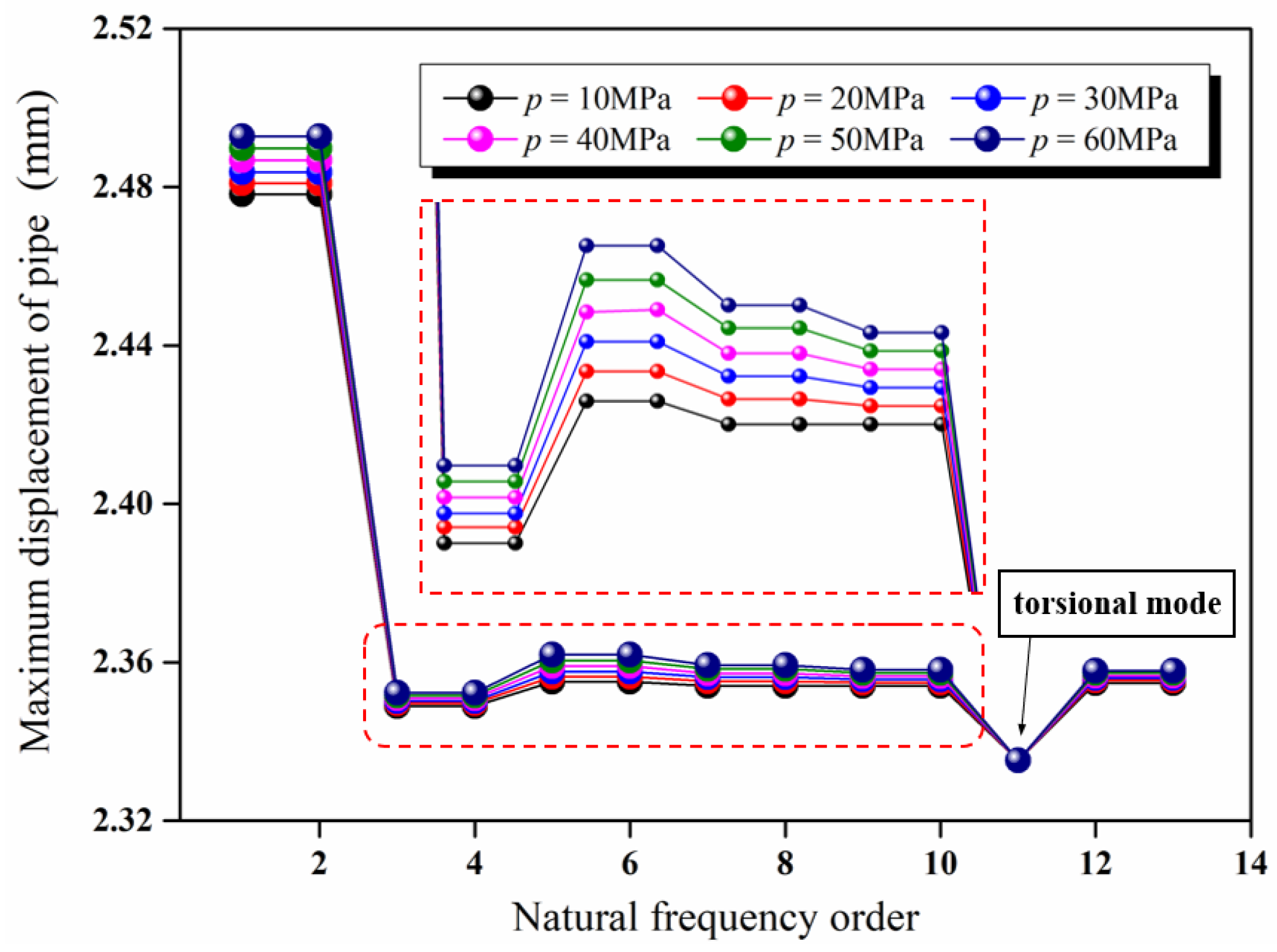
Figure 16.
Maximum displacement of tubing under different temperatures.
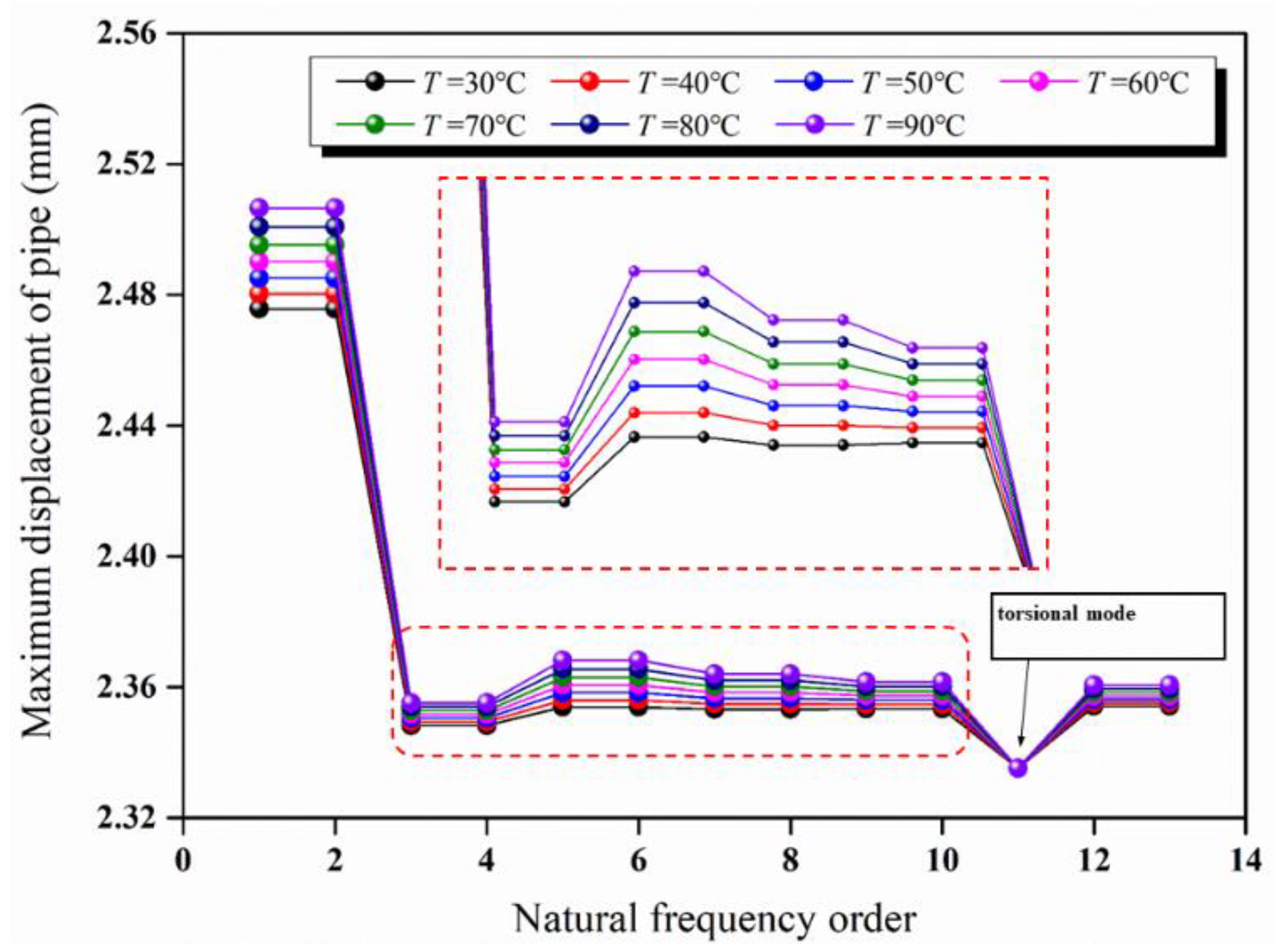
Figure 17.
Stress intensity and strain of tubing at different temperatures.

Table 1.
Natural frequencies of tubing under different inlet pressures (considering the fluid-structure interaction effect).
Table 1.
Natural frequencies of tubing under different inlet pressures (considering the fluid-structure interaction effect).
| Order | 10 MPa | 20 MPa | 30 MPa | 40 MPa | 50 MPa | 60 MPa |
|---|---|---|---|---|---|---|
| 1 | 10.891 | 10.604 | 10.308 | 10.003 | 9.6872 | 9.3599 |
| 2 | 10.891 | 10.604 | 10.308 | 10.003 | 9.6872 | 9.3599 |
| 3 | 30.721 | 30.346 | 29.966 | 29.581 | 29.19 | 28.793 |
| 4 | 30.721 | 30.346 | 29.966 | 29.581 | 29.19 | 28.793 |
| 5 | 60.477 | 60.071 | 59.662 | 59.250 | 58.836 | 58.418 |
| 6 | 60.477 | 60.071 | 59.662 | 59.251 | 58.836 | 58.418 |
| 7 | 99.550 | 99.124 | 98.697 | 98.268 | 97.837 | 97.404 |
| 8 | 99.550 | 99.125 | 98.697 | 98.268 | 97.837 | 97.404 |
| 9 | 147.46 | 147.02 | 146.58 | 146.14 | 145.69 | 145.25 |
| 10 | 147.46 | 147.02 | 146.58 | 146.14 | 145.69 | 145.25 |
| 11 | 163.00 | 162.97 | 162.95 | 162.92 | 162.89 | 162.86 |
| 12 | 203.67 | 203.22 | 202.76 | 202.31 | 201.86 | 201.40 |
| 13 | 203.67 | 203.22 | 202.76 | 202.31 | 201.86 | 201.40 |
| 14 | 263.03 | 263.03 | 263.04 | 263.04 | 263.05 | 263.05 |
Table 2.
Natural frequencies of tubing under different inlet pressures (fluid-structure interaction effect is not considered).
Table 2.
Natural frequencies of tubing under different inlet pressures (fluid-structure interaction effect is not considered).
| Order | 10 MPa | 20 MPa | 30 MPa | 40 MPa | 50 MPa | 60 MPa |
|---|---|---|---|---|---|---|
| 1 | 11.249 | 10.973 | 10.688 | 10.395 | 10.093 | 9.7807 |
| 2 | 11.249 | 10.973 | 10.688 | 10.395 | 10.093 | 9.7807 |
| 3 | 31.198 | 30.829 | 30.455 | 30.077 | 29.693 | 29.303 |
| 4 | 31.198 | 30.829 | 30.455 | 30.077 | 29.693 | 29.303 |
| 5 | 60.994 | 60.592 | 60.187 | 59.779 | 59.368 | 58.954 |
| 6 | 60.994 | 60.592 | 60.187 | 59.779 | 59.368 | 58.954 |
| 7 | 100.09 | 99.669 | 99.244 | 98.817 | 98.388 | 97.958 |
| 8 | 100.09 | 99.669 | 99.244 | 98.817 | 98.388 | 97.958 |
| 9 | 148.02 | 147.58 | 147.14 | 146.70 | 146.26 | 145.82 |
| 10 | 148.02 | 147.58 | 147.14 | 146.70 | 146.26 | 145.82 |
| 11 | 163.01 | 162.98 | 162.95 | 162.93 | 162.90 | 162.87 |
| 12 | 204.24 | 203.79 | 203.34 | 202.89 | 202.43 | 201.98 |
| 13 | 204.24 | 203.79 | 203.34 | 202.89 | 202.43 | 201.98 |
| 14 | 263.01 | 263.02 | 263.02 | 263.03 | 263.04 | 263.04 |
Table 3.
Natural frequencies of tubing under different inlet pressures (considering the fluid-structure interaction effect).
Table 3.
Natural frequencies of tubing under different inlet pressures (considering the fluid-structure interaction effect).
| Order | 30 °C | 40 °C | 50 °C | 60 °C | 70 °C | 80 °C | 90 °C |
|---|---|---|---|---|---|---|---|
| 1 | 11.152 | 10.677 | 10.178 | 9.6502 | 9.0894 | 8.4884 | 7.8379 |
| 2 | 11.152 | 10.677 | 10.178 | 9.6502 | 9.0894 | 8.4884 | 7.8379 |
| 3 | 31.068 | 30.443 | 29.803 | 29.149 | 28.478 | 27.790 | 27.083 |
| 4 | 31.068 | 30.443 | 29.803 | 29.149 | 28.478 | 27.790 | 27.084 |
| 5 | 60.854 | 60.177 | 59.492 | 58.799 | 58.098 | 57.388 | 56.669 |
| 6 | 60.854 | 60.177 | 59.492 | 58.800 | 58.098 | 57.388 | 56.669 |
| 7 | 99.946 | 99.238 | 98.525 | 97.807 | 97.084 | 96.354 | 95.620 |
| 8 | 99.946 | 99.239 | 98.525 | 97.807 | 97.084 | 96.355 | 95.620 |
| 9 | 147.87 | 147.14 | 146.41 | 145.67 | 144.93 | 144.19 | 143.44 |
| 10 | 147.87 | 147.14 | 146.41 | 145.67 | 144.93 | 144.19 | 143.44 |
| 11 | 163.03 | 163.02 | 163.00 | 162.99 | 162.98 | 162.97 | 162.95 |
| 12 | 204.09 | 203.34 | 202.60 | 201.84 | 201.09 | 200.34 | 199.58 |
| 13 | 204.09 | 203.34 | 202.60 | 201.85 | 201.09 | 200.34 | 199.58 |
| 14 | 263.02 | 263.04 | 263.05 | 263.07 | 263.08 | 263.10 | 263.12 |
Publisher’s Note: MDPI stays neutral with regard to jurisdictional claims in published maps and institutional affiliations. |
© 2022 by the authors. Licensee MDPI, Basel, Switzerland. This article is an open access article distributed under the terms and conditions of the Creative Commons Attribution (CC BY) license (https://creativecommons.org/licenses/by/4.0/).
Share and Cite
MDPI and ACS Style
Duan, J.; Li, C.; Jin, J. Modal Analysis of Tubing Considering the Effect of Fluid–Structure Interaction. Energies 2022, 15, 670. https://doi.org/10.3390/en15020670
AMA Style
Duan J, Li C, Jin J. Modal Analysis of Tubing Considering the Effect of Fluid–Structure Interaction. Energies. 2022; 15(2):670. https://doi.org/10.3390/en15020670
Chicago/Turabian StyleDuan, Jiehao, Changjun Li, and Jin Jin. 2022. "Modal Analysis of Tubing Considering the Effect of Fluid–Structure Interaction" Energies 15, no. 2: 670. https://doi.org/10.3390/en15020670
Note that from the first issue of 2016, this journal uses article numbers instead of page numbers. See further details here.