
Variable Incremental Controller of Permanent-Magnet Synchronous Motor for Voltage-Based Flux-Weakening Control


1
Department of Electrical Engineering, Gachon University, Seongnam-si 13120, Korea
2
Korea Railroad Research Institute, Uiwang-si 16105, Korea
*
Author to whom correspondence should be addressed.
Energies 2022, 15(15), 5733; https://doi.org/10.3390/en15155733
Submission received: 5 July 2022
/
Revised: 3 August 2022
/
Accepted: 5 August 2022
/
Published: 7 August 2022
(This article belongs to the Section F3: Power Electronics)
Abstract
:This study presents a variable incremental controller for flux-weakening control in the high-speed operation area of a permanent-magnetic synchronous motor (PMSM). In general, voltage-based flux-weakening control utilizes a reference voltage and a PI controller to generate a flux component current. In this paper, the voltage-based flux-weakening control is performed using the variable incremental controller instead of the PI controller. The variable incremental controller can control the flux component current using only the maximum speed and maximum current of the motor. A method for properly setting an appropriate variable incremental controller using acceleration is additionally presented. A variable incremental controller is applied and, accordingly, the overshoot of the motor speed can be reduced and the speed error of the motor can be minimized by reducing the difference between the actual motor and targeted accelerations. This method can simplify the design of a controller that utilizes flux-weakening control and can be applied to railroad cars whose acceleration does not alter frequently to increase the effect of motor control.
1. Introduction
To minimize environmental pollution caused by the utilization of fossil fuels, various policies are being established to efficiently produce and consume energy, such as low-carbon and green energy use [1,2]. In particular, recently, to address the environmental pollution challenge of machinery propelled using fossil fuels, such as automobiles, railways, and ships, such machinery has been replaced by electric motors [3,4,5,6,7].
Various motors are utilized in propulsion systems depending on their purpose or capacity, such as induction motors (IMs), synchronous motors (SMs), and brushless DC motors (BLDCs). Recently, various studies have been conducted using permanent-magnet synchronous motors (PMSMs), which have the advantages of high efficiency, high power density, and high reliability compared to other motors [8,9,10,11,12].
Various electric motors utilized in propulsion systems must have high-speed operation capabilities that exceed the rated speed when necessary [13,14]. Regarding PMSMs, high-speed operation is enabled using flux-weakening control, which reduces the effective magnetic flux size in the air gap, by generating a magnetic flux in the direction opposite to the magnetic flux direction [15,16,17]. Various studies on flux-weakening control have been conducted for the high-speed operation of motors. Initially, a method for reducing the magnetic flux component current in inverse proportion to the rotor speed was employed [18]; however, this method has a disadvantage, in that it is difficult to sufficiently utilize the voltage required for vector control, and the vector control is not accurate; thus, the efficiency of the motor drive may be reduced.
To address these limitations and perform accurate motor speed control, an optimal current control method with voltage- and current-limiting conditions has been proposed [19,20]. In this method, the magnitude of maximum voltage that can be applied to the motor, and the magnitude of maximum current that can flow through the motor are expressed in a current limit circle and voltage limit circle. By determining the most appropriate current point to drive the motor to control speed, the user can obtain a sufficient output torque capability of the motor. In addition, a method of conducting various experiments on the motor and creating the characteristics of the lookup table to control the motor is utilized [21,22,23]. However, this method has limitations, in that accurate information on the parameters is necessary because it is sensitive to changes in the motor parameters, and the control design is complicated because the variation characteristics of the motor must be considered. To address these challenges, various control methods using voltage feedback that are less affected by motor parameters have been studied [24,25]. Among them, voltage-based flux-weakening control for controlling magnetic flux has been studied [26,27]. In this method, control to weaken the magnetic flux is performed using the magnitude of the voltage applied to the motor. This method has the advantage of being robust against change factors because it does not adopt motor parameters. However, because feedback is formed between the reference voltage and voltage applied to the motor, a controller capable of minimizing error values is required [28,29,30].
Accordingly, in this study, a variable incremental controller is applied instead of the PI controller generally used for voltage-based flux-weakening control. The variable incremental controller has a different structure from the general PI controller. The variable incremental controller can control the flux component current using only the maximum speed and maximum current of the motor. In addition, this study presents a method for tuning an appropriate constant using the parameters and acceleration of the motor, rather than a fixed constant when using an incremental controller. As a result of applying a variable incremental controller to the voltage-based flux-weakening control, the overshoot of the motor speed can be reduced compared to the general method, and the speed error of the motor can be minimized by reducing the difference between the actual motor and targeted accelerations.
This paper is organized as follows. Section 2 describes the algorithm for the basic voltage-based flux-weakening control in detail. In addition, Section 2 describes an algorithm that applies a variable incremental controller to the voltage-based flux-weakening control. Section 3 describes the method for designing the fluctuation constant employed in the variable incremental controller and analyzes the effect through simulations. In Section 4, an experiment is conducted to verify the effectiveness of the variable incremental controller, and the results are analyzed. Finally, Section 5 concludes the paper.
2. Analysis of the Application of Voltage-Based Flux-Weakening Control According to the Controller
2.1. Application of Voltage-Based Flux-Weakening Control Using a PI Controller
In recent times, vector control has mainly been utilized to control electric motors. Vector control is a method employed to alter the three-phase voltage and current that changes over time into time-invariant voltage and current components, to control each component and enable precise speed control as instantaneous control of the motor speed.
Figure 1 illustrates a block diagram of a typical vector control utilized in synchronous motors with the voltage-based flux-weakening control method. Vector control measures the three-phase current flowing into the synchronous motor and converts it into d-axis (magnetic flux) current and q-axis (torque) current components using the DQ transform. The current components converted as such create an error between the d-axis and q-axis current references necessary for the synchronous motor to reach the targeted speed, and also control the torque of the synchronous motor by creating a voltage-manipulated variable through the PI controller. In the area where the motor operates at high speeds, the performance of the motor varies depending on the algorithm applied to the flux-weakening control block.
In this study, a voltage-based flux-weakening control and method are applied to maximize the magnitude of voltage applied to the motor without being affected by the motor parameters. When this method is applied, the voltage can be controlled even in a certain overmodulation area through voltage feedback. However, the design is complicated as the PI controller needs to be designed using various motor parameters [29]. Accordingly, in this paper, an incremental controller is used instead of a general PI controller to simplify the design of a controller that utilizes flux-weakening control.
2.2. Voltage-Based Flux-Weakening Control Using Variable Incremental Controller
In this study, flux-weakening control is performed through the voltage feedback structure, as illustrated in Figure 1, and an incremental controller is utilized to control the voltage-type controlled variable with the reference () of the current component [28].
As illustrated in Figure 2, the target amount, controlled variable, sensed voltage, and current values adopted in voltage and current controllers are generally converted into units of p.u. based on the magnitudes of the maximum voltage, current, and speed. Because the maximum controlled variable between the voltage and current values is the same, a current reference can be generated through voltage feedback, using an incremental controller. The incremental controller used as shown in Figure 2 is based on the algorithm of voltage-based flux-weakening control. Accordingly, even if the incremental controller is used, the range of flux-weakening region is the same as that of the voltage-feedback-based flux-weakening control. The algorithm of the variable incremental controller can be examined in detail as follows:
Figure 3 illustrates the algorithm flow chart of proposed variable incremental controller. Before driving the motor, the incremental constant () is calculated using the motor’s acceleration, maximum current, and maximum speed. is calculated only when the acceleration changes.
Unlike the PI controller, the variable incremental controller performs control using . The incremental controller comprises two stages. It determines whether is positive or negative when compared to zero, and can alter the current reference by adding or subtracting an incremental constant (). The calculation formula for is expressed in Equation (1) below:
According to Equation (1), is the difference between the magnitudes of the reference voltage () and calculated voltage (). A case where is greater than zero indicates a case where the reference voltage is greater than the calculated voltage, and may be considered to indicate that the voltage has not reached the maximum voltage. In this case, an incremental constant () should be added to the current reference () to increase the magnetic flux component current. An important point is that cannot have a value greater than 0, because the current of the magnetic flux component in a synchronous motor must always exist solely at a negative magnitude.
A case where is smaller than 0 indicates that the reference voltage is smaller than the calculated voltage, and it can be considered that the voltage exceeds the maximum voltage. Therefore, the d-axis reference current () should be reduced by an incremental constant () to reduce the current of the magnetic flux component. An important point here is that must be greater than −1 p.u. owing to the current limit circle, as the current of the magnetic flux component in the synchronous motor is normalized into units of p.u.
In the case of an incremental controller, the selection of the magnitude of is most important, as the performance of the controller is dependent on this magnitude. If voltage-feedback-based flux-weakening control is performed using an inappropriate magnitude of , various issues may arise.
In the case where the magnitude of is small, cannot maintain the command speed change rate; thus, the speed control response is reduced. In addition, because cannot keep up with the command speed change rate, overshoot may occur in the speed change, thereby deteriorating the stability of speed control.
In the case where the speed is controlled in the weak magnetic flux region when the magnitude of has been set to large, great current ripples may occur because the value of is large. This becomes a cause that can lead to oscillations in the target speed. Accordingly, the setting of an appropriate is the most important factor in designing a voltage feedback control, and this study proposes a method that can set the .
3. Voltage-Based Flux-Weakening Control Applied with the Proposed Variable Incremental Controller
3.1. Derivation of
To use the variable incremental controller, it is necessary to perform flux-weakening control with an optimal value according to the conditions, rather than a fixed value. As examined above, of the incremental controller must have a magnitude that produces as much change as acceleration. The formula for calculating that must be considered for the design of the variable incremental controller is as follows:
where:
- (p.u.)—Normalized maximum d-axis current;
- (rpm)—Maximum motor speed;
- (rpm)—Flux-weakening start speed;
- (Hz)—Motor acceleration;
- (Hz)—Calculation period.
means the normalized maximum magnitude of the current component injected when flux-weakening control of the motor is carried out and has the same meaning as the magnitude of the maximum current of the magnetic flux component. If the maximum current that can be supplied to the motor to be used is set to , and normalized into , and the magnitude of the normalized current is limited to 1/2 to prevent burnout of the motor that occurs as the current used for flux-weakening control increases, the magnitude can be calculated as follows:
means the maximum speed set when the high-speed operation algorithm for the motor was designed. can be set to a value within the maximum speed that can be achieved while using the flux-weakening control.
means the speed at which begins to have a negative (−) value and means the speed at which the flux-weakening control begins. It also means the speed at which begins to become larger than . Using SPMSM’s current limit circle and maximum volta ge current circle, can be set as follows:
To use the , the graph as illustrated in Figure 4 should be considered. Assuming that the time periods required to reach and according to the acceleration () and amount of change of , respectively, are the same, then the value of will not increase, such that the time for the motor to reach the speed can be reduced, overshoot can be reduced, and the ripple value in the steady state can be minimized. Accordingly, as illustrated in Figure 4, because the time between and can be obtained by dividing the speed difference between and by acceleration (), it can be expressed as Equation (5).
Because the time to reach according to the acceleration () should be the same as the time to reach according to the amount of change per second () in , an equation can be established by assuming () as an unknown number, as expressed in Equation (6) below.
denotes the amount of change in per second and * denotes the amount of change per second in the calculated frequency (). The expression can finally be expanded for considering as follows:
3.2. Simulation of Voltage-Feedback-Based Flux-Weakening Control Applied with the Proposed Variable Incremental Controller
Simulations were conducted to verify the performance of the variable incremental controller according to the change in acceleration and , as well as to compare and analyze the results. The motor utilized in the simulation was the SPMSM model, and its parameters were set as follows.
The magnitudes of calculated with parameters of the motor in Table 1 and the constant of the variable incremental controller were calculated, and the acceleration of the motor is presented in Table 2.
Figure 5 illustrates various graphs when the command speed is 7500 rpm and is . From Figure 5a, which is the speed graph of the motor, it can be observed that the time to reach the target command speed varies according to *. When is , it can be observed that the slope of the speed increment becomes smaller from the point where the flux-weakening control begins. As aforementioned, this is the result of the inability of the magnitude of to keep up with the speed change. Therefore, from Figure 5d, it can be observed that the magnitude of is increased after the flux-weakening control to reach the command speed.
However, from the command speed when , Figure 6a shows that there is no change in the slope of the amount of change in speed even after the flux-weakening control area. Accordingly, it can be observed that the command speed is reaches faster than when is adopted as .
However, regarding after reaching the target command speed in Figure 6c, it can be observed that the magnitude of the ripple of is higher than the magnitude of the ripple when is adopted as . That is, it can be observed that as increases, the speed overshoot until reaching the command speed decreases, but the current ripple after reaching the command speed increases.
Observing the command speed when is adopted as the obtained through the optimal calculation method for , Figure 7a shows that there is no change in the slope of the amount of change in speed even after the flux-weakening control area. In addition, regarding after the target command speed is reached in Figure 7c, it can be observed that the magnitude of the ripple of is lower than when is adopted as .
In other words, if voltage-based flux-weakening control is employed for the proposed variable incremental controller, the speed ripple can be minimized while reducing the overshoot of the speed to a minimum, using only the minimum required until the command speed is reached. Representatively, the result when the command speed is 2000 rpm is summarized in Table 3.
Figure 8 shows various waveforms when the flux-weakening control is performed using the PI controller, as shown in Figure 1, and when the flux-weakening control is performed with the proposed method as shown in Figure 2. Figure 8a shows various waveforms until the motor speed reaches the target speed of 7500 rpm. As a result, the proposed variable incremental controller can confirm the performance similar to that when using the PI controller. Figure 8b shows various waveforms when the load of the motor is changed in a situation where the speed of the motor is 7500 rpm. With the PI controller, it can be seen that the d-axis current is controlled in a curved shape. When the proposed flow incremental controller is used, it can be seen that the d-axis current is controlled in a straight shape. However, it has been confirmed that the speed and torque waveforms have almost the same shape, and it can be judged that the proposed variable incremental controller can perform flux-weakening control as with using the PI controller.
4. Experiment and Analysis
Experiments were conducted to demonstrate the practical effects of the incremental variable controller employed in the simulation. The parameters of the motor adopted in the experiment were the same as those adopted in the simulation (Table 1). The PMSM used was Texas Instruments’ HVPMSMMTR model, and the motor drive inverter module used the TMDSHVMTRINSPIN model. The equipment was configured as shown in Figure 9 and the experiment was conducted. The parameters of Inverter, Controller, and Motor used in the experiment were all the same as the constants shown in Table 1. All data of the experiment were measured by computer through SCI communication. To prove the effectiveness of the variable incremental controller in-depth, various experiments were conducted using acceleration. The magnitudes of adopted by acceleration were set as presented in Table 2 when the experiments were conducted.
Figure 10 illustrates various graphs when the command speed is 7500 rpm and is . From Figure 10a, which is the speed graph of the motor, it can be observed that the speed gradient decreases at the beginning of the flux-weakening control, in the time to reach the target command speed according to the acceleration. Except when the acceleration is 1000 rpmps, it can be observed that the speed gradient is not constant at all accelerations. In addition, from Figure 10b, it can be observed that speed overshoots occur in all acceleration areas, and the value of the speed increases up to 7856 rpm. Therefore, an overshoot that is approximately 4.74% higher than the command speed 7500 rpm occurs. From Figure 10d, because the maximum value of is measured to be about 0.31 p.u., a great change in is measured following the setting of a low . That is, even in actual experiments, the use of low results in high overshoots and significant changes in .
Figure 10 illustrates various graphs when the command speed is 7500 rpm and is . From Figure 11a, which is the speed graph of the motor, it can be observed that the times required to reach the target command speed according to the acceleration are minimum. This can be observed because of the fact that the magnitude of is sufficient to follow the speed command in time. Therefore, from Figure 11b, it can be observed that the overshoot of the speed is minimized in all acceleration areas, and the value of the speed increases up to 7530 rpm. Therefore, an overshoot of approximately 0.4% higher than the command speed 7500 rpm occurs, so the overshoot decreases compared to when is set to .
As illustrated in Figure 11d, as the maximum value of is measured to be approximately 0.03 p.u., an ideal result without any change in is indicated; however, as illustrated in Figure 11c, the maximum ripple of is approximately 0.037 p.u., which is larger than when is adopted as .
Figure 11 illustrates the resulting graphs when the command speed is 7500 rpm, and the values of calculated as the optimal values according to the acceleration are used. From Figure 12a, which is the speed graph of the motor, it can be observed that the times to reach the target command speed according to the acceleration are minimum. This can be observed because the magnitude of is not sufficient to follow the speed command in time. Therefore, from Figure 12b, it can be observed that the overshoots of the speed are minimized in all acceleration areas, and the value of the speed that increases up to 7537 rpm is measured. Therefore, an overshoot of approximately 0.49% higher than the command speed 7500 rpm occurs so that the overshoot decreases, compared to when is set to
As illustrated in Figure 12d, as the maximum value of is measured to be approximately 0.039 p.u., the change in is significantly reduced compared to when is adopted as . Therefore, as illustrated in Figure 10c, the maximum ripple of is approximately 0.028 p.u., which is smaller than when is used as .
In other words, when voltage-based flux-weakening control is employed for the proposed variable incremental controller, the speed and current ripples can be minimized while reducing the overshoot of the speed to a minimum, using only the minimum required until the command speed is reached, which could be experimentally verified.
5. Conclusions
This study presents a variable incremental controller for flux-weakening control in the high-speed operation area of a permanent-magnetic synchronous motor instead of the PI controller. The variable incremental controller can control the flux component current using only the maximum speed and maximum current of the motor. A measure to minimize the feedback errors by applying the incremental controller to the voltage-based flux-weakening control was adopted. A method to calculate the appropriate constants adopting the speed, current, and acceleration of the motor instead of a fixed constant when utilizing the incremental controller was presented.
Simulations and demonstration experiments were conducted to verify the superiority of the variable incremental controller. It was proven through various experiments that the variable incremental controller was able to reduce the speed overshoot by approximately 4% by tuning the . In addition, a tuned variable incremental controller was able to reduce the steady-state current ripples by approximately 24%. The variable incremental voltage-based flux-weakening control can be used for motor control using voltage feedback. This method can simplify the design of a controller that utilizes flux-weakening control. To increase the efficiency of motor control, it can be applied to railway vehicles with less frequent changes in acceleration than automobiles with frequent changes in acceleration.
Author Contributions
Conceptualization, H.L., G.L. and J.S.; methodology, H.L. and J.S.; resource, G.L. and G.K.; funding acquisition, G.L. and G.K.; software, H.L.; validation, J.S.; formal analysis, H.L.; writing—original draft preparation, H.L. and G.L.; project administration, G.K. and J.S.; writing—review and editing, H.L., G.L. and J.S.; supervision, J.S. All authors have read and agreed to the published version of the manuscript.
Funding
This research was supported by a grant from R&D Program (PK2203F1) of the Korea Railroad Research Institute and was supported by the Korea Institute of Energy Technology Evaluation and Planning (KETEP) and the Ministry of Trade, Industry & Energy (MOTIE) of the Republic of Korea (No. 20214000000060).
Institutional Review Board Statement
Not applicable.
Informed Consent Statement
Not applicable.
Data Availability Statement
Not applicable.
Conflicts of Interest
The authors declare no conflict of interest.
References
- The Government of the Republic of Korea. 2050 Carbon Neutral Strategy of the Republic of Korea towards a Sustainable and Green Society; The Government of the Republic of Korea: Seoul, Korea, 2020; pp. 16–17.
- Sustainable Development Solutions Network. America’s Zero Carbon Action Plan; Sustainable Development Solutions Network: New York, NY, USA, 2020; p. 27. [Google Scholar]
- Hasoun, M.; El Afia, A.; Chikh, K.; Khafallah, M.; Benkirane, K. A PWM Strategy for Dual Three-Phase PMSM Using 12-Sector Vector Space Decomposition for Electric Ship Propulsion. In Proceedings of the 19th IEEE MELECON, Marrakech, Morocco, 2–7 May 2018; pp. 243–248. [Google Scholar] [CrossRef]
- Ronanki, D.; Williamson, S.S. A Simplified Space Vector Pulse Width Modulation Implementation in Modular Multilevel Converters for Electric Ship Propulsion Systems. IEEE Trans. Trans. Elect. 2019, 5, 335–342. [Google Scholar] [CrossRef]
- Sieklucki, G. Optimization of Powertrain in EV. Energies 2021, 14, 725. [Google Scholar] [CrossRef]
- Stanescu, A.; Mocioi, N.; Dimitrescu, A. Hybrid Propulsion Train with Energy Storage in Metal Hydrides. In Proceedings of the Electric Vehicles International Conference (EV), Bucharest, Romania, 3–4 October 2019; pp. 1–4. [Google Scholar] [CrossRef]
- Yao, M.; Qin, D.; Zhou, X.; Zhan, S.; Zeng, Y. Integrated optimal control of transmission ratio and power split ratio for a CVT-based plug-in hybrid electric vehicle. Mech. Mach. Theory 2019, 136, 52–71. [Google Scholar] [CrossRef]
- Pillay, P.; Knshnan, R. Modeling of Permanent Magnet Motor Drives. IEEE Trans. Ind. Electron. 2008, 55, 2246–2257. [Google Scholar] [CrossRef] [Green Version]
- Tong, W.; Dai, S.; Wu, S.; Tang, R. Performance Comparison Between an Amorphous Metal PMSM and a Silicon Steel PMSM. IEEE Trans. Magn. 2019, 55, 8102705. [Google Scholar] [CrossRef]
- Fang, S.; Liu, H.; Wang, H.; Yang, H.; Lin, H. High Power Density PMSM with Lightweight Structure and High-Performance Soft Magnetic Alloy Core. IEEE Trans. Appl. Supercond. 2019, 29, 0602805. [Google Scholar] [CrossRef]
- Fan, W.J.; Zhu, X.Y.; Quan, L.; Wu, W.Y.; Xu, L.; Liu, Y.F. Flux-Weakening Capability Enhancement Design and Optimization of a Controllable Leakage Flux Multilayer Barrier PM Motor. Trans. Ind. Electron. 2021, 68, 7814–7825. [Google Scholar] [CrossRef]
- Jeong, M.T.; Lee, K.B.; Pyo, H.Y.; Nam, D.W.; Kim, W.H. A Study on the Shape of the Rotor to Improve the Performance of the Spoke-Type Permanent Magnet Synchronous Motor. Energies 2021, 14, 3785. [Google Scholar] [CrossRef]
- Gerada, D.; Mebarki, A.; Brown, N.L.; Gerada, C.; Cavagnino, A.; Boglietti, A. High-speed electrical machines: Technologies, trends, and developments. IEEE Trans. Ind. Electron. 2014, 61, 2946–2959. [Google Scholar] [CrossRef]
- Ahn, J.H.; Han, C.; Kim, C.W.; Choi, J.Y. Rotor design of high-speed permanent magnet synchronous motors considering rotor magnet and sleeve materials. IEEE Trans. Appl. Supercond. 2018, 28, 5201504. [Google Scholar] [CrossRef]
- Chen, Y.Z.; Huang, X.Y.; Wang, J.; Niu, F.; Zhang, J.; Fang, Y.T.; Wu, L.J. Improved Flux-Weakening Control of IPMSMs Based on Torque Feedforward Technique. IEEE Trans. Power. Electron. 2018, 33, 10970–10978. [Google Scholar] [CrossRef]
- Deng, T.; Su, Z.H.; Li, J.Y.; Tang, P.; Chen, X.; Liu, P. Advanced Angle Field Weakening Control Strategy of Permanent Magnet Synchronous Motor. IEEE Trans. Veh. Technol. 2019, 68, 3424–3435. [Google Scholar] [CrossRef]
- Zhang, X.A.; Foo, G.H.B.; Rahman, M.F. A Robust Field-Weakening Approach for Direct Torque and Flux Controlled Reluctance Synchronous Motors with Extended Constant Power Speed Region. IEEE Trans. Ind. Electron. 2020, 67, 1813–1823. [Google Scholar] [CrossRef]
- Xu, X.; Novotny, D.W. Selecting the flux reference for induction machine drives in the field weakening region. IEEE Trans. Ind. Appl. 1992, 28, 1353–1358. [Google Scholar] [CrossRef]
- Kim, S.H.; Sul, S.K. Maximum Torque Control of an Induction Machine in the Field Weakening Region. IEEE Trans. Ind. Appl. 1995, 31, 787–794. [Google Scholar] [CrossRef]
- Ye, M.T.; Shi, T.N.; Wang, H.M.; Li, X.M.; Xia, C.L. Sensorless-MTPA Control of Permanent Magnet Synchronous Motor Based on an Adaptive Sliding Mode Observer. Energies 2019, 12, 3773. [Google Scholar] [CrossRef] [Green Version]
- Wang, M.Z.; Sun, D.; Zheng, Z.H.; Nian, H. A Novel Lookup Table Based Direct Torque Control for OW-PMSM Drives. IEEE Trans. Ind. Electron. 2021, 68, 10316–10320. [Google Scholar] [CrossRef]
- Lee, D.Y.; Lee, J.H. Compensation of Interpolation Error for Look-Up Table-Based PMSM Control Method in Maximum Power Control. Energies 2021, 14, 5526. [Google Scholar] [CrossRef]
- Lee, D.Y.; Lee, J.H. Low Cost Simple Look-Up Table-Based PMSM Drive Considering DC-Link Voltage Variation. Energies 2020, 13, 3904. [Google Scholar] [CrossRef]
- Jacob, J.; Bottesi, O.; Calligaro, S.; Petrella, R. Design Criteria for Flux-Weakening Control Bandwidth and Voltage Margin in IPMSM Drives Considering Transient Conditions. IEEE Trans. Ind. Appl. 2021, 57, 4884–4900. [Google Scholar] [CrossRef]
- Miguel-Espinar, C.; Heredero-Peris, D.; Gross, G.; Llonch-Masachs, M.; Montesinos-Miracle, D. Maximum Torque per Voltage Flux-Weakening Strategy with Speed Limiter for PMSM Drives. IEEE Trans. Ind. Electron. 2021, 68, 9254–9264. [Google Scholar] [CrossRef]
- Sepulchre, L.; Fadel, M.; Pietrzak-David, M.; Porte, G. MTPV Flux-Weakening Strategy for PMSM High Speed Drive. IEEE Trans. Ind. Appl. 2018, 54, 6081–6089. [Google Scholar] [CrossRef]
- Dong, Z.; Yu, Y.; Li, W.; Wang, B.; Xu, D. Flux-Weakening Control for Induction Motor in Voltage Extension Region: Torque Analysis and Dynamic Performance Improvement. IEEE Trans. Ind. Electron. 2018, 65, 3740–3751. [Google Scholar] [CrossRef]
- Lee, H.J.; Shon, J.G. Improved Voltage Flux-weakening Strategy of Permanent Magnet Synchronous Motor in High-speed Operation. Energies 2021, 14, 7464. [Google Scholar] [CrossRef]
- Zhang, Y.; Jin, J.; Jiang, H.; Jiang, D. Adaptive PI Parameter of Flux-Weakening Controller Based on Voltage Feedback for Model Predictive Control of SPMSM. In Proceedings of the 2020 IEEE Energy Conversion Congress and Exposition (ECCE), Detroit, MI, USA, 11–15 October 2020; pp. 2674–2681. [Google Scholar] [CrossRef]
- Kim, S.H.; Sul, S.K. Voltage Control Strategy for Maximum Torque Operation of an Induction Machine in the Field-Weakening Region. IEEE Trans. Ind. Electron. 1997, 44, 512–518. [Google Scholar] [CrossRef]
Figure 1.
Block diagram of typical voltage-based flux-weakening control.

Figure 2.
Block diagram of voltage-based flux-weakening control when using an incremental controller.
Figure 2.
Block diagram of voltage-based flux-weakening control when using an incremental controller.

Figure 3.
Algorithm flowchart of the proposed variable incremental controller.
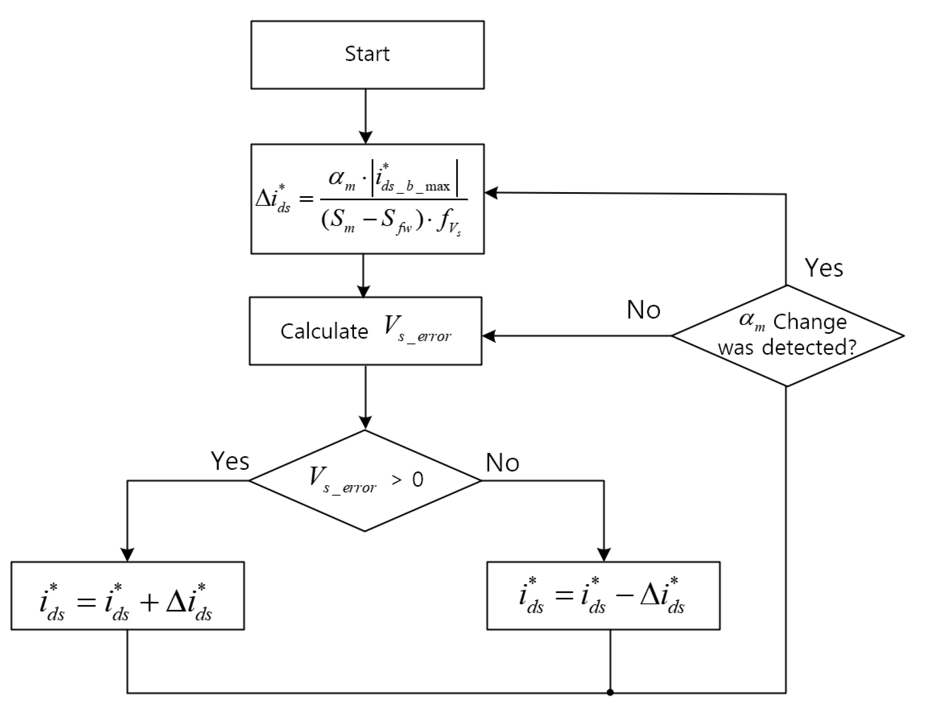
Figure 4.
Ideal graphs of speed and for the design of variable incremental controllers.
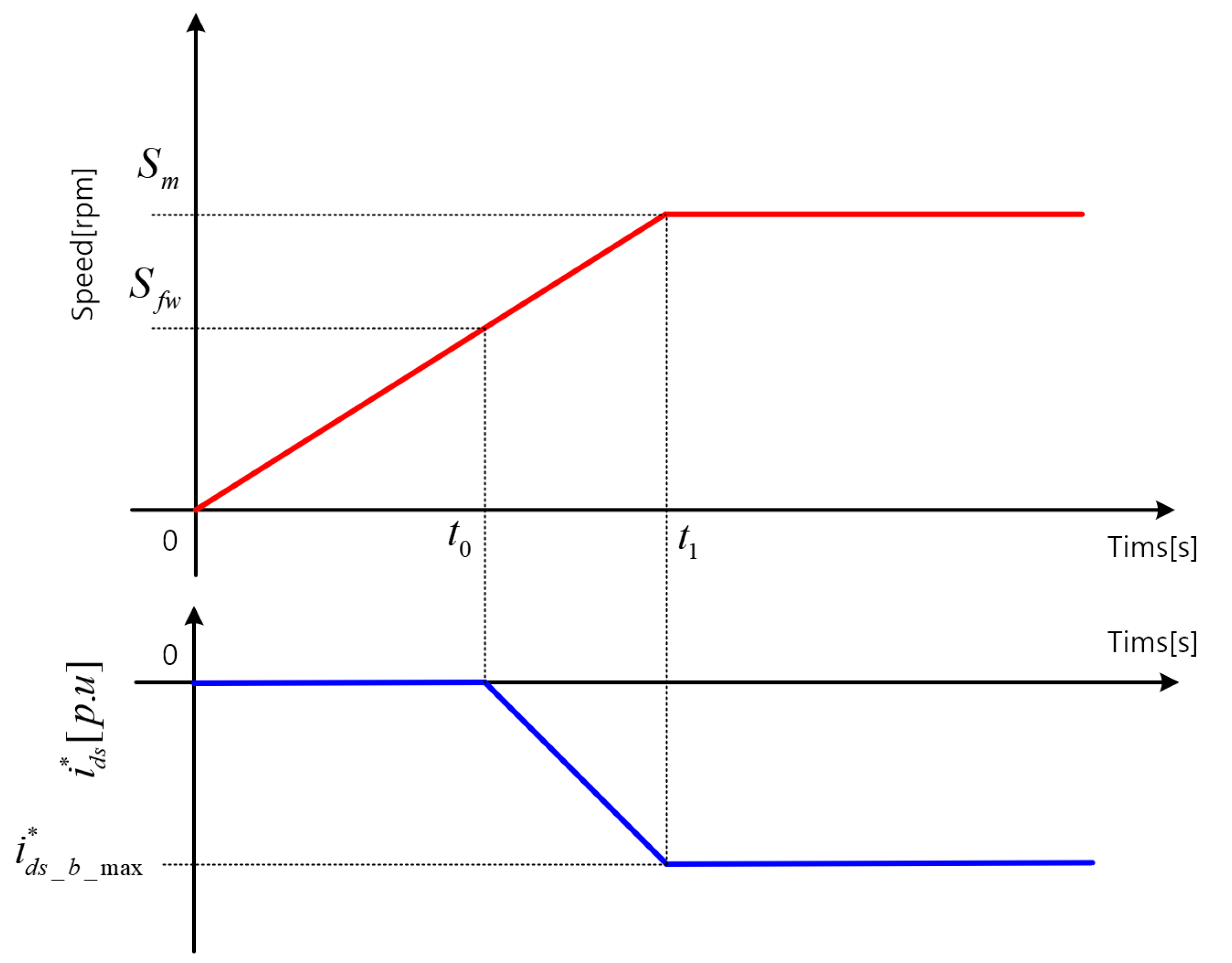
Figure 5.
Simulation results when is : (a) motor speed; (b) motor speed; (c) d-axis current; (d) q-axis current.
Figure 5.
Simulation results when is : (a) motor speed; (b) motor speed; (c) d-axis current; (d) q-axis current.
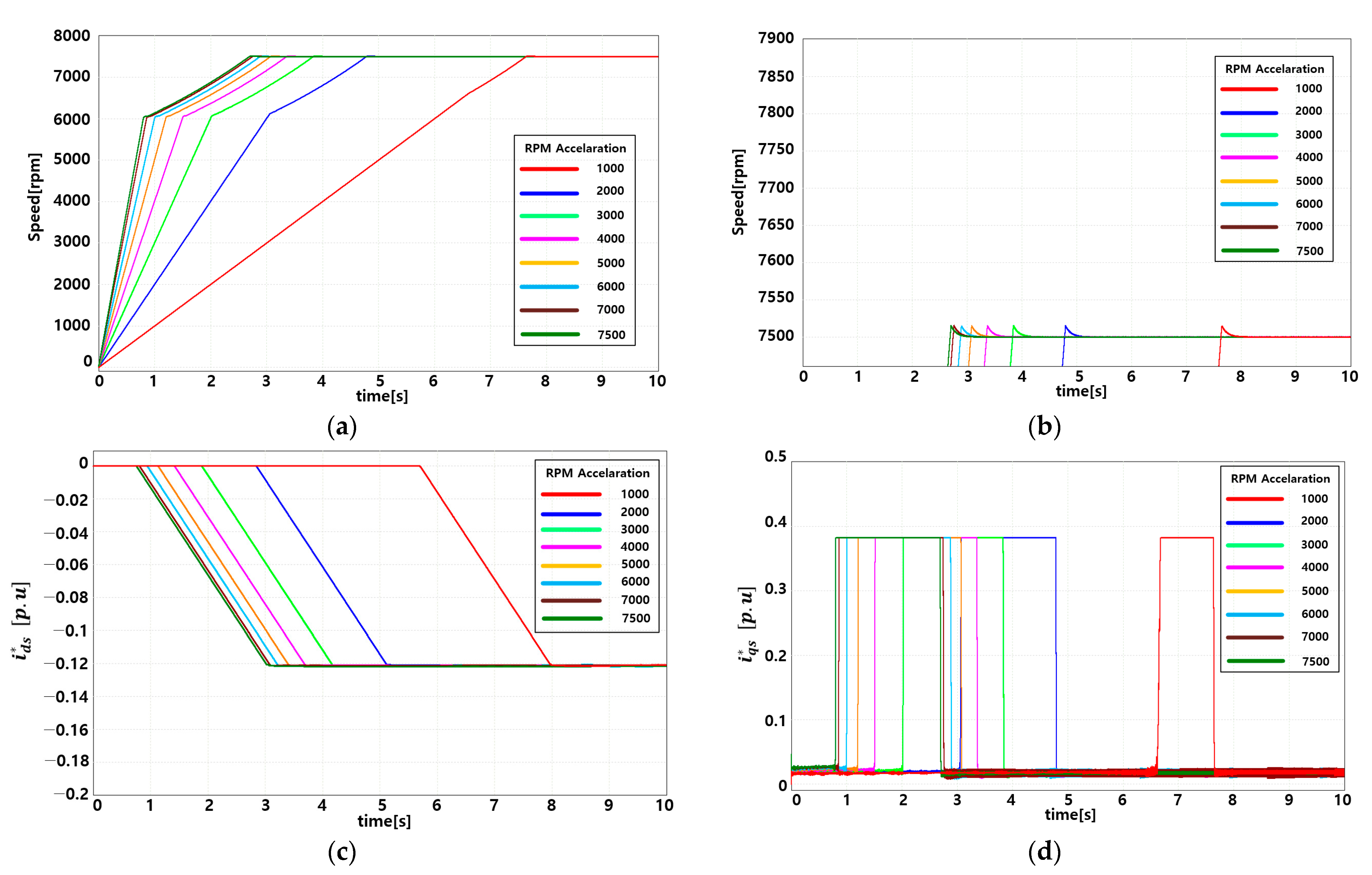
Figure 6.
Simulation results when is : (a) motor speed; (b) motor speed; (c) d-axis current; (d) q-axis current.
Figure 6.
Simulation results when is : (a) motor speed; (b) motor speed; (c) d-axis current; (d) q-axis current.
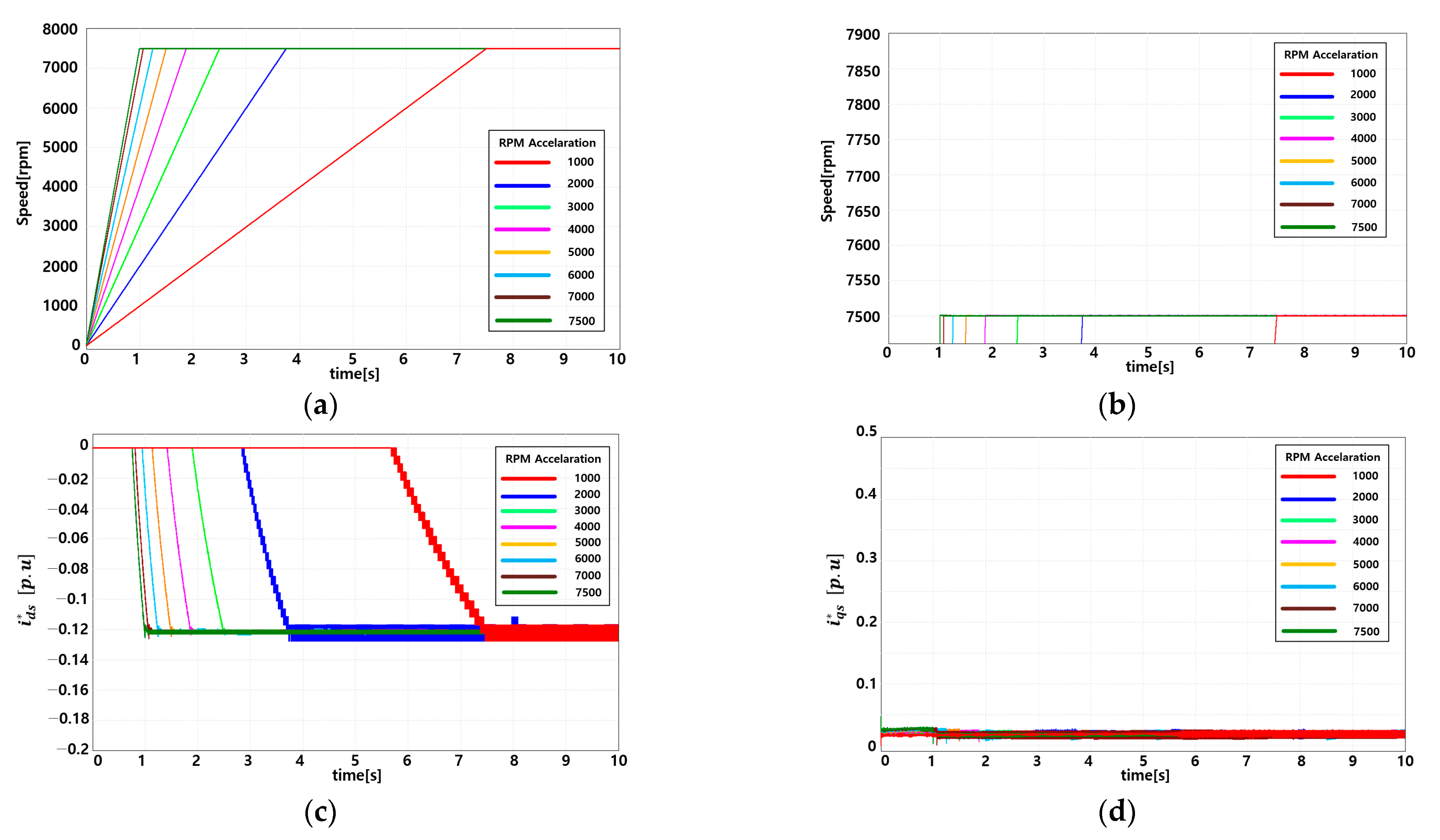
Figure 7.
Simulation results when is optimized: (a) motor speed; (b) motor speed; (c) d-axis current; (d) q-axis current.
Figure 7.
Simulation results when is optimized: (a) motor speed; (b) motor speed; (c) d-axis current; (d) q-axis current.
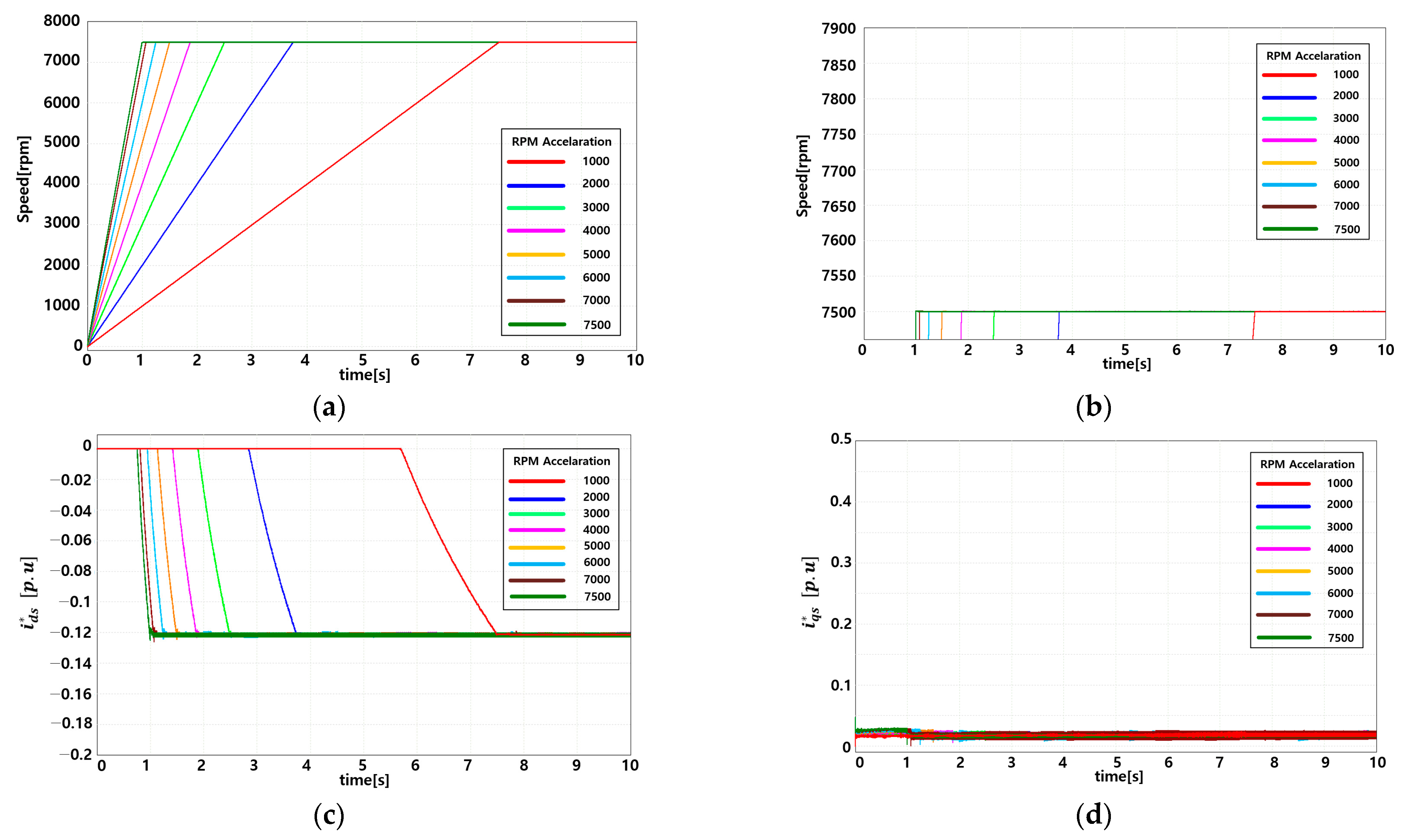
Figure 8.
Simulation results according to controller: (a) waveform of the process to reach target speed; (b) when the torque of the motor changes.
Figure 8.
Simulation results according to controller: (a) waveform of the process to reach target speed; (b) when the torque of the motor changes.
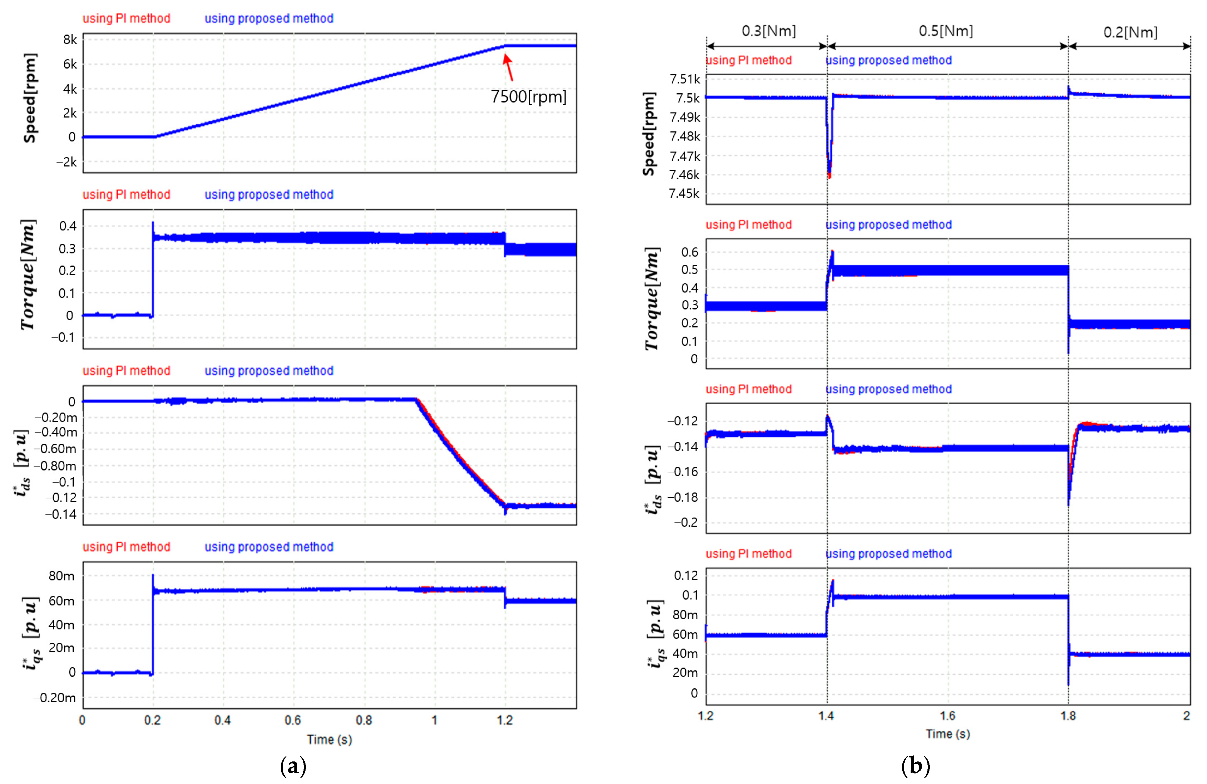
Figure 9.
The experimental environment: (a) 4-channel oscilloscope; (b) control board and inverter; (c) SPMSM; (d) current and voltage probes; (e) personal computer.
Figure 9.
The experimental environment: (a) 4-channel oscilloscope; (b) control board and inverter; (c) SPMSM; (d) current and voltage probes; (e) personal computer.
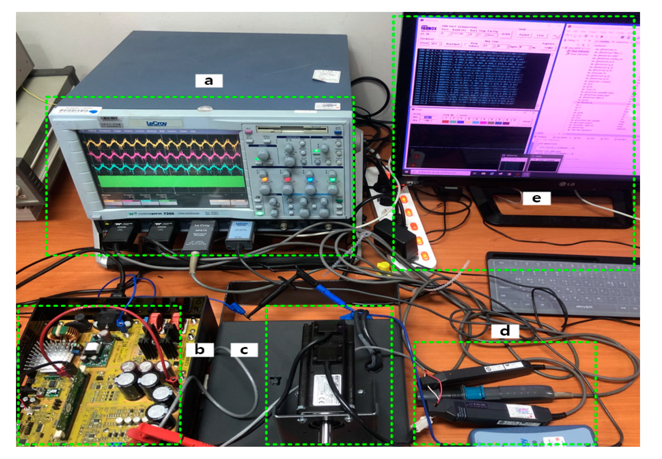
Figure 10.
Experimental results when is : (a) motor speed; (b) motor speed; (c) d-axis current; (d) q-axis current.
Figure 10.
Experimental results when is : (a) motor speed; (b) motor speed; (c) d-axis current; (d) q-axis current.
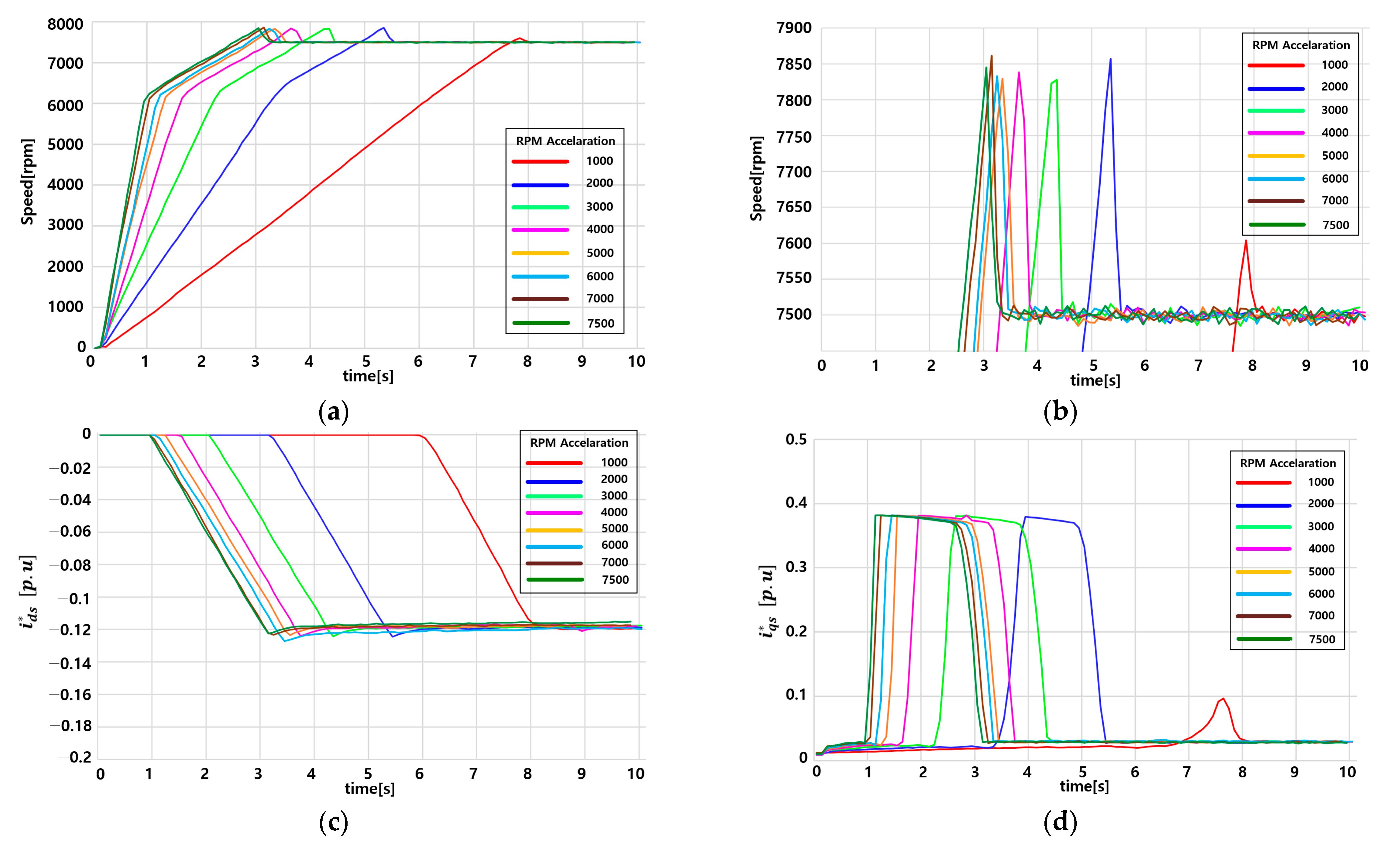
Figure 11.
Experimental results when is : (a) motor speed; (b) motor speed; (c) d-axis current; (d) q-axis current.
Figure 11.
Experimental results when is : (a) motor speed; (b) motor speed; (c) d-axis current; (d) q-axis current.

Figure 12.
Experimental results when is optimized: (a) motor speed; (b) motor speed; (c) d-axis current; (d) q-axis current.
Figure 12.
Experimental results when is optimized: (a) motor speed; (b) motor speed; (c) d-axis current; (d) q-axis current.


Table 1.
Summary of various parameters used in the simulations.
| Device | Parameter | Unit | Value |
|---|---|---|---|
| Inverter | DC-LINK voltage | (V) | 290 |
| Max current | (A) | 3.82 | |
| Switching frequency | (Hz) | 20,000 | |
| Motor | Back EMP(Ke) | (Vpk/krpm) | 49 |
| Number of poles | (P) | 8 | |
| Resistance | (Ω) | 2.2 | |
| Inductance | (H) | 0.0109 | |
| Inertia | (oz-in-s2) | 0.00439 |
Table 2.
Summary of various parameters adopted in the simulations.
| RPM Reference (rpm) | RPM Acceleration (rpmps) | |||
|---|---|---|---|---|
| 7500 | 1000 | |||
| 2000 | ||||
| 3000 | ||||
| 4000 | ||||
| 5000 | ||||
| 6000 | ||||
| 7000 | ||||
| 7500 |
Table 3.
Summary of simulation results when speed command is 2000 rpm.
| (Unit) | ||||
|---|---|---|---|---|
| 2.672 × 10⁻⁴ | 5.34 × 10⁻⁵ | 1.068 × 10⁻⁴ | ||
| Speed Arrival Time | (s) | 4.78 | 3.75 | 3.75 |
| Speed max. Overshoot | (rpm) | 7515 | 7500 | 7500 |
| ripple | (p.u.) | 0.000053 | 0.0106 | 0.000641 |
| (p.u.) | 0.381 | 0.0271 | 0.0243 | |
| ripple | (p.u.) | 0.00647 | 0.0165 | 0.0065 |
Publisher’s Note: MDPI stays neutral with regard to jurisdictional claims in published maps and institutional affiliations. |
© 2022 by the authors. Licensee MDPI, Basel, Switzerland. This article is an open access article distributed under the terms and conditions of the Creative Commons Attribution (CC BY) license (https://creativecommons.org/licenses/by/4.0/).
Share and Cite
MDPI and ACS Style
Lee, H.; Lee, G.; Kim, G.; Shon, J. Variable Incremental Controller of Permanent-Magnet Synchronous Motor for Voltage-Based Flux-Weakening Control. Energies 2022, 15, 5733. https://doi.org/10.3390/en15155733
AMA Style
Lee H, Lee G, Kim G, Shon J. Variable Incremental Controller of Permanent-Magnet Synchronous Motor for Voltage-Based Flux-Weakening Control. Energies. 2022; 15(15):5733. https://doi.org/10.3390/en15155733
Chicago/Turabian StyleLee, Hyunjae, Gunbok Lee, Gildong Kim, and Jingeun Shon. 2022. "Variable Incremental Controller of Permanent-Magnet Synchronous Motor for Voltage-Based Flux-Weakening Control" Energies 15, no. 15: 5733. https://doi.org/10.3390/en15155733
Note that from the first issue of 2016, this journal uses article numbers instead of page numbers. See further details here.