Exergy Analysis of the Prevailing Residential Heating System and Derivation of Future CO₂-Reduction Potential

Abstract

The residential heating sector accounts for a large share of the worldwide annual primary energy consumption. In order to reduce CO₂-emissions, it is therefore particularly important to analyse this sector for potential efficiency improvements. In Europe, natural gas boilers are the most widely used heating technology since they are cost-effective and can be installed in any type of building. The energy efficiency of these boilers is already high. However, in their internal process, heat is generated at a high temperature level which is only used for space heating and therefore a high amount of exergy remains unused. This research aims to develop the potential of using the exergy to further improve the efficiency of the systems. A novel combination of methods is applied to analyse the thermodynamic behaviour of gas-fired boilers in detail and over the cycle of a year. The analysis is performed in two steps: In the first step a system is examined in stationary operating points. This is carried out through an experimental setup and a three-dimensional numerical simulation. In the second step, the obtained data is applied to a transient annual building simulation. The results show the temporal distribution and total amount of the annual exergy loss for a common residential building. The exergy loss accumulates to 16,271 kWh per year, which shows the high potential to partially convert the exergy to electrical energy and significantly reduce the external electricity demand and CO₂-emissions of the building. Based on this, new technologies such as Thermoelectric Generators can be developed, which can enable this potential.

1. Introduction

To mitigate climate change the CO₂-emissions of all energy sectors need to be reduced. This includes the development of renewable energy sources and the overall improvement of efficiency. The European energy policy framework also addresses these goals by its road-map to maximize the beneftis from energy efficiency and maximize the deployment of renewable energies [1]. An important sector for this decarbonization is the residential heating sector. In Europe, it accounts for around 3000 TWh/year or 16% of the total primary energy consumption [2]. The most used primary energy source is natural gas with a share of $44\%$ [2] from which $86\%$ is used in individual boilers. This is followed according to their share by biomass, oil, coal, nuclear energy, renewable energy and waste [2]. Possible reasons for the widespread use of gas-fired boilers are their cost-effectiveness of operation and investment and the possibility of installation in any type of building.

The thermal efficiency of modern gas-fired condensing boilers is already high. The research to further improve their efficiency focusses on the optimization of their operation conditions, by which an efficiency of over $99\%$ can be reached [3]. Furthermore, their corrosion resistance is analysed to keep up the energy efficiency over a longer period of time [4] or the possibility to retrofit systems with a lower energy efficiency to improve the overall efficiency is regarded [5].

A possibility to decarbonize gas-fired boilers is to use a different fuel than natural gas. A suitable substitution is hydrogen, produced from renewable energy sources. The hydrogen may be produced with a surplus of renewable energy from photovoltaic power plants in summer and stored for the use in winter. The advantage is that a continuos transition is possible as the existing infrastructure can be used and 10–20% hydrogen can be mixed in with the natural gas [6]. Analysis of the mixture combustion conditions show that the lowest emissions appear with a hydrogen volume fraction of $24.7\%$ [7]. This development is underlined by novel commercially available hydrogen ready boilers [8]. However, the possible future scarcity of hydrogen and the currently still low exergetic efficiency of the boilers need to be considered as well. Also biogas produced from waste or other residues is one of the promising renewable gas sources.

The exergetic efficiency specifies the ratio between the used and the produced exergy. In boilers the fuel is burned at high temperatures with high exergy and used to heat water at low temperatures with near zero exergy. To improve the exergetic efficiency a part of the high temperature heat needs to be converted to electrical energy. However, existing technologies like Organic Rankine Cycle power plants are mainly used for the application in district heating [9] and are too investment-intensive and complex for individual residential use.

The advantages to improve the exergetic efficiency are clarified by regarding the current costs and emissions of heat from natural gas and grid electricity, for example for the year 2021 in Germany as shown in

Table 1. Costs and emissions of heat from natural gas and grid electricity for recent years in Germany.

Energy	Costs (€/kWh)	Emissions (kg/kWh)
Heat from natural gas	0.07 [10]	0.25 [11]
Grid electricity	0.32 [12]	0.38 [13]

. This depicts that the conversion of exergy from heat to electricity reduces the energy cost by 0.25 €/kWh and the emissions by 0.13 kg/kWh.

Thermoelectric Generators (TEGs) have the potential to convert the exergy loss in residential boilers to electrical energy and significantly reduce the electricity demand and CO₂ emissions of the building. TEGs convert heat directly into electricity based on the Seebeck-Effect. Therefore, they are almost maintenance free, compact, silent in operation and cost-effective even in small-scale applications such as boilers. Their potential is already demonstrated in the waste heat recovery of passenger cars [14,15,16] and commercial vehicle applications [17,18]. The technical feasibility for the use in boilers is also already shown [19,20]. However, to further optimize the integration an in-depth knowledge of the thermodynamic processes is needed.

There are studies analyzing the exergy of residential heating systems and especially of natural gas boilers [21]. The studies find that the exergy loss is up to 96.2% for conventional boilers [22] and between 92.9% [23] and 96.6% [24] for condensing boilers. The values depend on environmental factors such as the outdoor temperature, which is used as the minimum temperature in the exergy calculation. These studies focus on the exergy loss on building level at discrete steps such as primary exergy input, heat generation and distribution. Further research is needed regarding the detailed spatial distribution of thermal properties within the system as a basis for future developments.

This study aims to provide a foundation for the future development in utilization of the exergy in residential heating systems. Therefore, an in-depth analysis of a modern gas-fired boiler as a reference system is performed. The aforementioned research gap is closed by a novel combined analysis. The analysis consists of an experimental setup that measures the system in stationary operating points. The experiment is accompanied by a three-dimensional numerical simulation, that quantifies the spatial distribution of fluid flows, temperatures and heat flows in more detail. The combined results are used in a one-dimensional transient annual building simulation. This shows the resulting thermodynamic condition of the system throughout a year that can be used for future development and optimization of new technologies. These technologies can significantly reduce the CO₂-emissions of the heating sector in an economic way.

2. Methodology

The approach of this study is based on three methods. The thermodynamic behaviour of the system in stationary operation points is analysed with an experimental setup and a three-dimensional numerical simulation. The obtained results are used in a one-dimensional building simulation. All methods are described in the following.

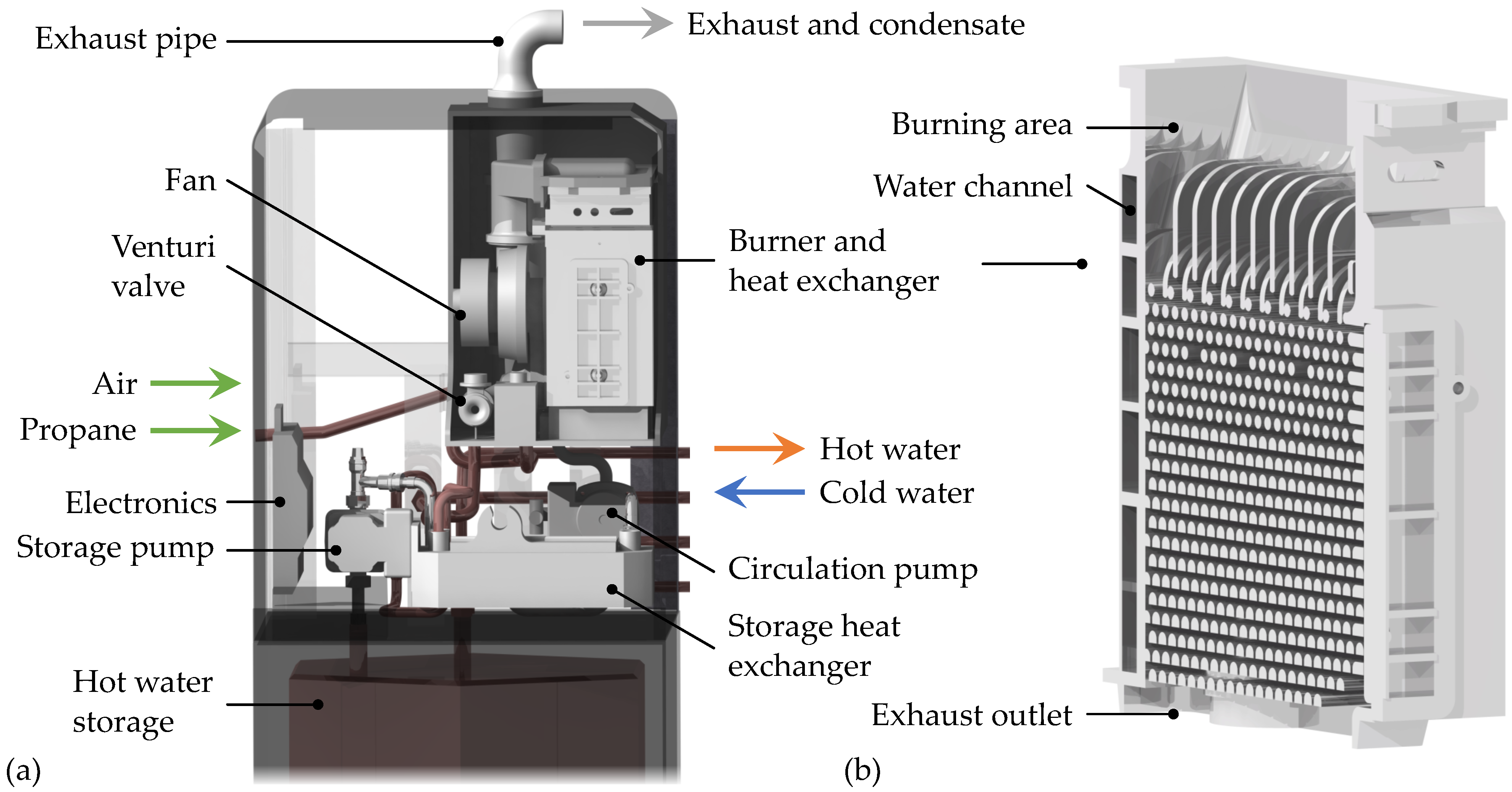
2.1. Experimental Setup of the Boiler

The regarded system is a Bosch Condens GC9000i WM20/100 S condensing boiler [25]. It is supplied with propane and has a nominal heat output of 20 kW_th with a maximum seasonal space heating thermal energy efficiency of 94%.

The composition of the boiler is shown in Figure 1a. Pressurized propane (P) flows into the system and draws in air via a venturi valve. Both gases are transported by a fan into a burner, where the mixture is ignited. The burner and heat exchanger are one integrated component and shown in a detailed sectional view in Figure 1b. The hot gas (HG) flows through the fins of the heat exchanger and heat is transferred to water in housing-channels in a counter-flow arrangement. The hot gas leaves the heat exchanger as exhaust gas and condensate via pipes. Additionally, the system has a 100 L storage tank for hot drinking water. The tank can be loaded with the storage pump and the storage heat exchanger, which transfer heat from the water of the main heat exchanger to the water in the storage tank. A heating buffer storage can be externally connected to the system as well.

In the experiment, the heat in the water is dissipated to a cooling system, which represents the radiators in a house. The temperature of the returning cold water (CW) is kept constant at $T_{CW}=303$ K. The hot water storage is not used in the experiment, as it does not influence the behaviour of the burner and heat exchanger. An external heating buffer storage is not connected for the same reasons. The heat output of the system is varied from 4 kW_th to 20 kW_th in six operating points. The operating points are adjustable with with values from 10–60%. Each operating point is maintained until no relevant changes in the system are observed any more.

The experiment is implemented to analyse the thermodynamic behaviour of the system and to validate the three-dimensional heat exchanger simulation. The simulation is used for further analysis of heat flows or thermal radiation. For this purpose, important measures of the experiment are the temperature distribution and the mass flow of the propane, hot gas and the cold water.

The temperature distribution is measured with thermocouples. The position per configuration and type of the thermocouples in the hot gas heat exchanger is shown in Figure 2. Each configuration represents one measurement run which covers all operation points. The experimental process is divided into four configurations to minimize the influence of the thermocoupels on the system and on each other. The thermocouple type is selected based on the maximal expected temperature as shown in

Table 2. Specifications of the different types of thermocouples used in the experiment [26].

Type	Max. Temperature	Accuracy	Diameter
B	1973 K	±1.5 K or 0.0025 T	1.5 mm
S	1873 K	±1 K	1.5 mm
N	1573 K	±1.5 K or 0.004 T	1.5 mm
K	1473 K	±1.5 K or 0.004 T	1 mm

. The type K thermocouples are used to measure the water temperature and are distributed evenly in one side of the water channels.

The mass flow of the hot gas is measured with an mass air flow meter based on the hot wire anemometer principle. The sensor is placed in the exhaust pipe and has an accuracy of 3% [27]. The propane mass flow is measured indirectly. Next to the anemometer a lambda probe [28] is placed which measures the air-fuel ratio from which the propane mass flow can be calculated by

$${\dot{m}}_P=\frac{{\dot{m}}_A}{\lambda L_{st}},$$

(1)

where ${\dot{m}}_P$ is the mass flow of propane in kg/s, ${\dot{m}}_A$ is the mass flow of air in kg/s, $\lambda$ is the air-fuel ratio and $L_{st}$ = 15.57 kg_A/kg_P is the stoichiometric air requirement based on the chemical equation of the reaction. The volume flow of the water is measured by a magnetic inductive flow meter [29] with an accuracy of ±0.25%. The volume flow is converted to the mass flow by multiplying it with its density.

2.2. Three-Dimensional Heat Exchanger Simulation

To further understand the processes in the heat exchanger and to determine its exergy loss, a three-dimensional numerical model is developed. This is particularly important since the hot thermocouples are in heat radiation exchange with the cold wall. Therefore they only indicate the temperature of the thermocouple itself and not the temperature of the hot gas. The numerical model is used to determine the temperature of the hot gas and validated with the measured temperatures of the thermocouples.

The model is shown in Figure 3, it is simulated using the software ANSYS Fluent, ANSYS, Inc., Version 2021 R1, Canonsburg, PA, USA. A grid convergence study is performed and shows no further need for refinement of the computational grid. For simplification it is assumed that the physics of the heat exchanger are symmetrical in the y- and z-direction. This allows the reduction to a quarter of the actual heat exchanger geometry. Thermal heat transfer is calculated using energy equations and thermal radiation is modelled using the discrete ordinates radiation model. Latent heat from condensation is neglected as it only appears in the low temperature region and does not affect the exergy significantly.

The outer shell and inner pins of the heat exchanger are modelled as a solid part consisting of the aluminium alloy AlSi10Mg. The coolant liquid is modelled as a convective heat transfer boundary condition. Its heat transfer coefficient is approximated to ${\alpha }_{CW}=7000$ W/(m${}^2$ K) based on the experimental values. All other walls are modelled adiabatic.

The hot gas is modelled as a turbulent fluid flow with the material properties of exhaust gas and the k-$ϵ$-SST Model. In order to avoid complex modelling of the flame, the inlet is defined as a mass flow inlet with a specified temperature and an emission coefficient that represents the thermal radiation of the flame. The inlet parameters are based on the experimental data, additionally for the inlet temperature the equation

$${\dot{Q}}_{ce}={\dot{Q}}_{in,c}+{\dot{Q}}_{in,r},$$

(2)

is used, with heat of the combustion energy ${\dot{Q}}_{ce}$, convective inlet heat ${\dot{Q}}_{in,c}$ and radiant inlet heat ${\dot{Q}}_{in,r}$. With simplified equations inserted, this results in

$${\dot{m}}_P{H}_{i,p}=\sigma T_{in}^4{A}_{in}{ϵ}_{in}+{\dot{m}}_{in}{c}_{p,in}(T_{in}-T_0),$$

(3)

with the experimental values massflow of propane ${\dot{m}}_P$ and total inlet massflow ${\dot{m}}_{in}$ both in kg/s and the constant parameters lower heating value of propane $H_{i,p}$ = 46,390.1 kJ/kg, Stefan-Boltzmann constant $\sigma$, inlet surface area $A_{in}$ in m${}^2$, emissivity of the inlet ${ϵ}_{in}=0.22$ and ambient temperature $T_0=298$ K. The experimental values are adjusted according to the measurements of each operating point.

Comparable values are necessary to validate the temperatures of the simulation with the experiment. In the experimental setup thermocouples are used to measure the temperature. However, the thermocouples interact with the surrounding heat exchanger, for example by radiant heat transfer from the hot thermocouple to the cold heat exchanger. Therefore, the thermocouples in the hot regions of the setup show lower temperatures compared to the hot gas and cannot directly be compared with the simulated values of the hot gas. To obtain comparable data, the thermocouples themselves and their interaction are modelled, too. The thermocouples and their positions are based on the experimental configuration 2. The thermocouples are modelled with a thermal conductivity of ${\lambda }_{TC}$ = 70 W/(mK) based on the volume averaged values of their materials and an emissivity of ${ϵ}_{TC}=0.1$ based on blanked platinum, which is the protective shell material of the used type B thermocouples.

The overall aim of this study is to specify the exergy loss of the system. The exergy in the model is defined based on the Carnot efficiency

$$\dot{E}=\dot{Q}(1-\frac{T_H}{T_C}),$$

(4)

with the exergy $\dot{E}$ in W, the heat flow $\dot{Q}$ in W and the hot $T_H$ and the cold $T_C$ temperatures. The equation is used for radiant heat transfer as ${\dot{E}}_r$ based on the thermal radiation of the inlet and for the convective heat transfer as ${\dot{E}}_c$ based on the mass-weighted average temperatures of the flows ${\overline{T}}_{HG}$ and ${\overline{T}}_{CL}$ and the convective heat flow ${\dot{Q}}_c$. The latter is evaluated on planes with a constant coordinate x and is therefore a function of the coordinate x. The total exergy flow ${\dot{E}}_{tot}$ is defined as

$${\dot{E}}_{tot}={\dot{E}}_r+{\int }_{in}^{out}{\dot{E}}_{c}dx.$$

(5)

2.3. One-Dimensional Building Simulation

The building simulation is implemented in the program Dymola 2020. It consists of models of the open-source Modelica library AixLib [30]. The schematic view of the model is shown in Figure 4. It depicts the examined boiler from Section 2.1 and Section 2.2 in a typical detached house. The boiler model calculates the heat input from the burner ${\dot{Q}}_B$ and fuel consumption from efficiency values for each operation point. Depending on the current heat demand, the heat up water is used for space heating or to thermally load the hot water storage. If the heat demand exceeds the maximal possible heat input, the hot water supply is covered first.

The building parameters are obtained from tables based on a living space of 150 m${}^2$ in an existing building and a four person household [31]. Their temporal distributions are based on reference load profiles [32]. The total heat demand is divided into heat demand for space heating ${\dot{Q}}_{SH}$ and hot water ${\dot{Q}}_{HW}$. It is modeled for ten typical days of a year, which are combined depending on the climate conditions. Here, the days are combined according to climate zone 10 [33], which represents a middle-European location. The composed yearly heat demand is shown in Figure 5 with a time resolution of 15 min and as a daily mean value.

3. Results and Discussion

3.1. Stationary Analysis on Heat Exchanger Level

The heat exchanger is examined under constant boundary conditions per operating point using the experimental setup from Section 2.1 and the simulation from Section 2.2. Both methods are compared using the thermocouples of measurement configuration 2 to validate the simulation. Figure 6 shows this comparison over different operating points. The simulation results in no solution at the two lowest operating points, as the low velocities involved cause convergence problems. At the other operating points, the simulated temperatures of the thermocouples TC-172, TC-173 and TC-151 match well with the experiment. The highest deviation regarding these thermocouples is lower than ±5%.

The simulated temperatures of the thermocouples TC-171 and TC-152 do not match the experiment well. This is caused by simplifications of the simulation model compared to the real heat exchanger. Figure 7 shows the resulting temperatures of the simulation for the highest operating point. In (b) an detailed view of TC-171 is shown. The thermocouple is placed at the boundary layer of the inlet flow. Therefore, it is strongly affected by the condition of the inlet mass flow, e.g., its turbulence intensity or inflow angle. These conditions are not measured and are therefore not reproduced in the model, causing the deviation of TC-171. In Figure 7c a detailed view of the other deviating thermocouple is shown. It is placed under the second row of connected pins and on two symmetrical planes. This causes deviation, as the hot gas flow is not as symmetrical as assumed and does not flow on the pins directly.

To summarize the validation, important values close to the inlet and outlet of the simulation agree well with the experiment. The deviation of other values can be explained with model inaccuracy which do not affect the overall results significantly. Therefore, the simulation model is considered valid and used for further analysis.

Figure 8 shows the mass-weighted average temperature distribution along the coordinate x for the highest operating point, which is 60%. The hot gas temperature is obtained from the simulation, the coolant liquid temperature from the experiment. It shows the high inlet temperature and the fast heat transfer along the heat exchanger. The varying pin geometry causes the unsteadiness of the slope of the curve.

Furthermore, the according specific convective heat flow and exergy flow are shown on the right axis. The specification refers to the section of the coordinate x. Both values are also dependent on the pin geometry. The exergy close to the inlet is high and its proportion of the heat decreases with the temperature difference.

The convective heat and exergy flow and the radiant heat and exergy flow are then combined to the total heat and exergy flow, as described in Section 2.2. The results depending on the operating point are shown in Figure 9 and point out the high exergy losses. Factors for the high exergy loss of the system are the high operation temperature and the low space heating temperatures, which are inserted in Equation (4). For example at the operating point 60% around 19.2 kW heat is produced and 12.5 kW exergy are lost. This exergy loss shows the high potential to convert a part of it to electrical energy and reduce the external power requirements of the building significantly.

3.2. Transient Analysis on Building Level

In residential buildings, the heating system is not continuously operated with nominal heat output. It is operated depending on the heat demand of the building. Accordingly, the available exergy varies throughout the year. The analysis is expanded considering this circumstance using the model described in Section 2.3. The daily averaged results for the heat and exergy flow are shown in Figure 10.

The model shows that the daily averaged heat flow is closely correlated to the combined heat demand for room heating and hot water. That it because the boiler control is able to adjust the heat output proportionally to the heat demand. The hot water storage tank is only needed for short term peak loads.

The accumulated annual heat or thermal energy is 28,331 kWh and annual exergy loss is 16,271 kWh. Most of it is produced in the months of October to April, which is in about 58.3% of a year. For a four person household, 6000 kWh of electrical energy demand can be assumed which is roughly evenly distributed throughout the year [32]. This results in 3498 kWh electrical energy demand in the months of October to April. During these months, only 12.3% of the heat or 21.5 of the exergy in the home heating system need to be converted to electricity, to fully meet the demand. The potential of this conversion regarding Table 1 is 874.5 €/year cost reduction and 454.7 kg/year reduction of CO${}_2$-emissions. During the remaining time of the year a photovoltaic system can be used to further reduce the external electricity demand and related emissions.

The potential use of exergy in boilers also exists for the future use of natural gas and hydrogen mixtures. The sustainably and costly produced hydrogen or other gases like biogas and methane are then not only used for heating, but also for the supply of electricity. This increases the benefit of the overall process chain and the economy of renewable gases.

4. Conclusions

Among residential heating systems, gas-fired boilers are the prevailing technology with a market share of 44%. These boilers produce hot gas at high temperatures and heat water to low temperatures with a high exergy loss. This study examines the exergy loss in detail by experimental and simulative stationary analysis on heat exchanger level and transient analysis on building level. The stationary analysis shows good agreement between experiment and simulation. The results for the highest operating point show 12.5 kW exergy loss at 19.2 kW heat output. These results are then transferred to the transient simulation on building level for evaluation over the course of a year. The results are an annual heat output of 28,331 kWh and exergy loss of 16,271 kWh.

The presented results show a high potential to use the otherwise lost exergy in residential heating systems. A large part of the electricity demand of a household can be covered with it, with lower emissions compared to grid electricity. TEGs are a solution to this problem as they are able to recover a large part of the heat: 12.5% are needed to cover the whole electricity demand, current TEGs have efficiencies of up to 9% [18]. Therefore, current TEGs are already almost able to cover the whole electricity demand of a household in the months from October to April. Furthermore, they are compact in size and have potentially low investment costs. This makes them an economic and environmentally friendly solution for many buildings. Additionally, in the future, these systems can be combined with photovoltaic systems. The systems complement each other, as TEGs produce electricity in cold month with low solar radiation and photovoltaic systems produce electricity in month with high solar radiation.

To utilize the shown potential, further research and development of TEGs is needed. Especially a detailed optimization of the heat exchanger, considering all specific requirements of the integration in a gas-fired boiler. In addition, the admixture of hydrogen and biogas should be investigated to further reduce the emissions. In combination, an economic shift towards a renewable energy system is supported.

References

1. European Commission. A Clean Planet for All: A European Strategic Long-Term Vision for a Prosperous, Modern, Competitive and Climate Neutral Economy: COM(2018) 773 Final. 2018. Available online: https://eur-lex.europa.eu/legal-content/EN/TXT/PDF/?uri=CELEX:52018DC0773 (accessed on 30 April 2022).
2. Bertelsen, N.; Vad Mathiesen, B. EU-28 Residential Heat Supply and Consumption: Historical Development and Status. Energies 2020, 13, 1894. [Google Scholar] [CrossRef]
3. Fernández-Cheliz, D.; Velasco-Gómez, E.; Peral-Andrés, J.; Tejero-González, A. Energy Performance Optimization in a Condensing Boiler. Environ. Sci. Proc. 2021, 9, 6. [Google Scholar] [CrossRef]
4. Huang, X.; Sun, M.; Kang, Y. Fireside Corrosion on Heat Exchanger Surfaces and Its Effect on the Performance of Gas-Fired Instantaneous Water Heaters. Energies 2019, 12, 2583. [Google Scholar] [CrossRef] [Green Version]
5. Życzyńska, A.; Majerek, D.; Suchorab, Z.; Żelazna, A.; Kočí, V.; Černý, R. Improving the Energy Performance of Public Buildings Equipped with Individual Gas Boilers Due to Thermal Retrofitting. Energies 2021, 14, 1565. [Google Scholar] [CrossRef]
6. International Renewable Energy Agency. Hydrogen: A Renewable Energy Perspective. Available online: https://www.irena.org/-/media/Files/IRENA/Agency/Publication/2019/Sep/IRENA_Hydrogen_2019.pdf (accessed on 30 April 2022).
7. Xin, Y.; Wang, K.; Zhang, Y.; Zeng, F.; He, X.; Takyi, S.A.; Tontiwachwuthikul, P. Numerical Simulation of Combustion of Natural Gas Mixed with Hydrogen in Gas Boilers. Energies 2021, 14, 6883. [Google Scholar] [CrossRef]
8. Bosch Thermotechnik GmbH. One Step Closer to the Energy Transition: Bosch Presents Hydrogen Boiler for Residential Buildings. 2020. Available online: https://www.bosch-presse.de/pressportal/de/en/der-energiewende-einen-schritt-naeher-220800.html (accessed on 30 April 2022).
9. Gołębiewski, M.; Galant-Gołębiewska, M. Economic Model and Risk Analysis of Energy Investments Based on Cogeneration Systems and Renewable Energy Sources. Energies 2021, 14, 7538. [Google Scholar] [CrossRef]
10. Bantle, C. BDEW-Gaspreisanalyse Januar 2022. Available online: https://www.bdew.de/media/documents/220124_BDEW-Gaspreisanalyse_Januar_2022_24.01.2022_final_YTK8Nlb.pdf (accessed on 30 April 2022).
11. Mailach, B.; Oschatz, B. BDEW-Heizkostenvergleich Altbau 2017: Ein Vergleich der Gesamtkosten Verschiedener Systeme zur Heizung und Warmwasserbereitung in Altbauten. Available online: https://www.bdew.de/internet.nsf/res/24E1B62F814ADC3DC12580B30059CEB8/\protect\T1\textdollarfile/1_FINAL%20HKV-Altbau%202017.pdf (accessed on 13 June 2018).
12. Bantle, C. BDEW-Strompreisanalyse. Available online: https://www.bdew.de/media/documents/220504_BDEW-Strompreisanalyse_April_2022_04.05.2022.pdf (accessed on 30 April 2022).
13. Icha, P. Entwicklung der Spezifischen Kohlendioxid-Emissionen des Deutschen Strommix in den Jahren 1990–2020. Available online: https://www.umweltbundesamt.de/sites/default/files/medien/5750/publikationen/2021-05-26_cc-45-2021_strommix_2021_0.pdf (accessed on 30 April 2022).
14. Kober, M. Holistic Development of Thermoelectric Generators for Automotive Applications. J. Electron. Mater. 2020, 49, 2910–2919. [Google Scholar] [CrossRef] [Green Version]
15. Kober, M.; Knobelspies, T.; Rossello, A.; Heber, L. Thermoelectric Generators for Automotive Applications: Holistic Optimization and Validation by a Functional Prototype. J. Electron. Mater. 2020, 49, 2902–2909. [Google Scholar] [CrossRef] [Green Version]
16. Kober, M. The High Potential for Waste Heat Recovery in Hybrid Vehicles: A Comparison Between the Potential in Conventional and Hybrid Powertrains. J. Electron. Mater. 2020, 49, 2928–2936. [Google Scholar] [CrossRef] [Green Version]
17. Heber, L.; Schwab, J. Modelling of a thermoelectric generator for heavy-duty natural gas vehicles: Techno-economic approach and experimental investigation. Appl. Therm. Eng. 2020, 174, 115156. [Google Scholar] [CrossRef]
18. Heber, L.; Schwab, J.; Knobelspies, T. 3 kW Thermoelectric Generator for Natural Gas-Powered Heavy-Duty Vehicles—Holistic Development, Optimization and Validation. Energies 2022, 15, 15. [Google Scholar] [CrossRef]
19. Qiu, K.; Hayden, A.C.S. Development of Thermoelectric Self-Powered Heating Equipment. J. Electron. Mater. 2011, 40, 606–610. [Google Scholar] [CrossRef]
20. Zhang, Y.; Wang, X.; Cleary, M.; Schoensee, L.; Kempf, N.; Richardson, J. High-performance nanostructured thermoelectric generators for micro combined heat and power systems. Appl. Therm. Eng. 2016, 96, 83–87. [Google Scholar] [CrossRef] [Green Version]
21. Evola, G.; Costanzo, V.; Marletta, L. Exergy Analysis of Energy Systems in Buildings. Buildings 2018, 8, 180. [Google Scholar] [CrossRef] [Green Version]
22. Yildiz, A.; Güngör, A. Energy and exergy analyses of space heating in buildings. Appl. Energy 2009, 86, 1939–1948. [Google Scholar] [CrossRef]
23. Lohani, S.P. Energy and exergy analysis of fossil plant and heat pump building heating system at two different dead-state temperatures. Energy 2010, 35, 3323–3331. [Google Scholar] [CrossRef]
24. Baldi, M.G.; Leoncini, L. Effect of Reference State Characteristics on the Thermal Exergy Analysis of a Building. Energy Procedia 2015, 83, 177–186. [Google Scholar] [CrossRef] [Green Version]
25. Bosch Thermotechnik GmbH. Datenblatt Gas-Brennwertgerät Condens GC9000iWM. Technical Data Sheet. Available online: https://www.bosch-thermotechnology.com/ocsmedia/optimized/full/o342378v47_6720869212.pdf (accessed on 30 April 2022).
26. DIN EN 60584-1:2014-07; Thermoelemente–Teil 1: Thermospannungen und Grenzabweichungen (IEC_60584-1:2013); Deutsche Fassung EN_60584-1:2013. DIN Deutsches Institut für Normung e.V.: Berlin, Germany, 2014. [CrossRef]
27. Robert Bosch GmbH. Heißfilm-Luftmassenmesser. Technical Data Sheet. Available online: https://www.ibs-gruppe.de/shop/media/pdf/7f/45/6e/Datenblatt-0-280-218-119.pdf (accessed on 30 April 2022).
28. Robert Bosch GmbH. Sauerstoff-Lambda-Sonde LSU 4.9. Technical Data Sheet. Available online: https://www.ibs-gruppe.de/shop/media/pdf/72/3f/75/Datenblatt57c022628447c.pdf (accessed on 30 April 2022).
29. H. Hermann Ehlers GmbH. Magnetisch-Induktive Durchflussmesser. Technical Data Sheet. Available online: https://www.ehlersgmbh.com/media/pdf/Datenblaetter/Badger/DB-BA-MID-Uebersicht.pdf (accessed on 30 April 2022).
30. Müller, D.; Remmen, P.; Constantin, A.; Lauster, M.; Fuchs, M. AixLib—An Open-Source Modelica Library within the IEA-EBC Annex60 Framework. In Proceedings of the CESBP Central European Symposium on Building Physics and BauSIM 2016, Dresden, Germany, 14–16 September 2016. [Google Scholar]
31. Schweizerischer Ingenieur- und Architektenverein. Raumnutzungsdaten für die Energie- und Gebäudetechnik. 2015. Available online: http://shop.sia.ch/normenwerk/architekt/sia%202024/d/2015/D/Product (accessed on 30 April 2022).
32. Verein Deutscher Ingenieure. VDI 4655: Referenzlastprofile von Ein- und Mehrfamilienhäusern für den Einsatz von KWK-Anlagen. 2008. Available online: https://www.beuth.de/en/technical-rule/vdi-4655/105958871 (accessed on 30 April 2022).
33. DIN 4710:2003-01; Statistiken Meteorologischer Daten zur Berechnung des Energiebedarfs von heiz- und Raumlufttechnischen Anlagen in Deutschland. DIN Deutsches Institut für Normung e.V.: Berlin, Germany, 2003. [CrossRef]
Figure 1. (a) Composition of the condensing boiler and its interfaces; (b) Detailed sectional view of the integrated burner and heat exchanger of the system.
Energies 15 03502 g001
Figure 2. Position and type of the thermocouples in the hot gas heat exchanger in different configurations. The thermocouples of configuration 2 are labelled as they are used for the validation of the three-dimensional heat exchanger simulation.
Energies 15 03502 g002
Figure 3. Three-dimensional numerical model of the heat exchanger. It is reduced to a quarter of the actual geometry using symmetry planes. Solid parts are shown in gray, the hot gas flowing from the top to the bottom is shown in orange. The coolant liquid is modelled as a convective heat transfer boundary condition.
Energies 15 03502 g003
Figure 4. Schematic view of the modeled building energy system. It depicts the analyzed boiler in a typical detached house.
Energies 15 03502 g004
Figure 5. Heat demand of the modeled building for (a) space heating and (b) hot water over a year. The lighter colored values have a time resolution of 15 min per value, the darker colored values are daily averages.
Energies 15 03502 g005
Figure 6. Comparison of the experimental and simulated thermocouple temperatures. Markers represent the experiment and lines the simulation. The simulation model has a high accuracy at values depicted with solid lines and deviations for the dashed lines.
Energies 15 03502 g006
Figure 7. Results of the simulation for the highest operating point. (a) Overview of the model; (b) Detail view of the thermocouple TC-171; (c) Detail view of the thermocouple TC-152.
Energies 15 03502 g007
Figure 8. Spatial distribution of the mass-weighted average Temperature on the left axis and of the specific convective heat flow and according exergy flow on the right axis along the coordinate x for the highest operating point.
Energies 15 03502 g008
Figure 9. Total heat flow and total exergy flow depending on the operating point.
Energies 15 03502 g009
Figure 10. Daily averaged values of the heat flow and the exergy flow of the system in a residential building in the course of a year.
Energies 15 03502 g010