
A Resampling Slack-Based Energy Efficiency Analysis: Application in the G20 Economies


1
Teaching Center, Zhejiang Open University, 42 Jiaogong Road, Hangzhou 310012, China
2
Lifelong Education Institute, Zhejiang Open University, 42 Jiaogong Road, Hangzhou 310012, China
3
Department of Economics, Soochow University, No. 56, Section 1, Kueiyang Street, Chungcheng District, Taipei City 100, Taiwan
4
Center for General Education, National Open University, No.172, Zhongzheng Road, Luzhou District, Xinbei City 247031, Taiwan
5
Department of Applied Economics, Fo Guang University, No.160, Linwei Road, Jiaosi 262307, Taiwan
*
Author to whom correspondence should be addressed.
Energies 2022, 15(1), 67; https://doi.org/10.3390/en15010067
Submission received: 4 September 2021
/
Revised: 15 December 2021
/
Accepted: 16 December 2021
/
Published: 22 December 2021
(This article belongs to the Special Issue Energy Policy for a Sustainable Economic Growth)
Abstract
:In order to have a sustainable economic and social development, it is important to balance economic growth and ecological environmental damage. In this article, we used the resampling model under the triangular distribution to evaluate energy efficiency, because the input/output value may have measurement errors, time lag factors, arbitrariness, and other problems, causing their own DMU to change. After these factors were taken into consideration, the resampled input/output was estimated because a super-SBM efficiency value was placed in the confidence interval. From the past-present data, for the estimated data change, the time weight was provided according to the Lucas series, and the super-SBM was time-weighted. We applied this model to a dataset of G20 economies from 2010 to 2014. To the best of our knowledge, very few studies have applied the DEA method with resampling to analyze energy efficiency. Thus, our study contributes to the methodologies for energy efficiency evaluation. We found that the overall average energy efficiency is 0.653, with substantial differences between developed economies and developing economies. The most important finding is that neither overestimation nor underestimation occurred when sampling was repeated one thousand times using 95% and 80% confidence intervals, confirming the robustness of the super-SBM model. The less energy-efficient economies should adjust their energy policies appropriately and develop new clean energy technologies in the future.
1. Introduction
Climate change has drawn considerable global concern as a growing threat to humanity and ecosystems. According to a report by the Intergovernmental Panel on Climate Change in 2018, if carbon emissions continue to increase at the current rate, the Earth’s temperature will rise by more than 1.5 °C by 2030 to 2052, and, thus, the average sea level will rise by 0.26 to 0.77 m relative to sea levels in 2005. Accumulating evidence has strongly suggested that the global climate is changing as a result of human activities, particularly those that cause the release of greenhouse gases from fossil fuels; and given the fact that the world economy is still highly dependent on traditional energy sources, improving the energy efficiency is therefore critical to alleviating global climate change.
In recent years, a great deal of studies have paid attention to energy efficiency [1,2,3,4,5,6,7,8,9]. As for the measurement of energy efficiency, the DEA approach has been widely used so far [10,11,12,13,14,15,16,17,18,19,20,21,22,23,24,25,26,27,28,29,30,31,32,33,34]. DEA applies multiple inputs to yield multiple outputs in a given time period to evaluate the relative efficiency of an individual DMU from the distance of each DMU to the frontier [10]. This approach follows the model developed by Charnes, Cooper, and Rhodes and modified by Banker, Charnes, and Cooper (BCC) [11,12]. However, these models cannot process undesirable outputs, and the best efficiency is equal to one in multiple DMUs. As energy efficiency is related to environmental variables, it may be affected by undesirable outputs, such as CO2. Thus, it is necessary to obtain real efficiency scores when investigating energy policies [13]. As traditional DEA does not require special production functions, it is difficult to draw numerical inferences from DEA scores. Some studies have used bootstrap DEA to create confidence intervals [3], but this method does not provide information regarding changes in the states of inputs and outputs.
The resampling DEA approach solves the problem of input and output scores being subject to adjustments in measurement errors, hysteretic factors, and arbitrariness in efficiency scores [14,15,16]. Simar and Wilson proposed a general bootstrapping methodology for nonparametric frontier models [17] and then extended this method by allowing for heterogeneity in the efficiency structure [18]. Tone first proposed a nonradial, nonoriented efficiency estimation method for the SBM model and estimated efficiency scores between zero and one [14]. Then, he systematically proposed three resampling models in his work [19]. Subsequently, Fang et al. proposed a slack-based version of the super-SBM [20]. The resampling DEA method has been applied in various settings, such as the measurement of airport efficiencies [22], the investigation of technical efficiency indexes of banks [23], and the efficiency evaluation of the railway sector [29].
Although studies on the DEA measurement of energy efficiency are abundant, to the best of our knowledge, studies have only infrequently applied the resampling DEA approach to the assessment of energy use performance. To close this research gap, our study utilized the resampling SBM DEA method and the past-present model with resampling to evaluate the energy efficiencies of G20 economies. Our study contributes to the methodologies for the energy efficiency evaluation.
Our study took the members of G20 as DMU because G20 relies on accumulated experience to formulate effective measures to promote energy efficiency. According to the G20 Energy Efficiency Leading Programme, in the past few decades, especially from 1990 to 2013, G20 economies’ GDP energy consumption dropped by 1.4% annually, saving a total of 4.3 billion tons of oil consumption, equivalent to a reduction of 10.4 billion tons of CO2 emissions. As an important representative of the world economic system, G20 has taken the investment in energy efficiency as an important task. The amount of its investment in energy efficiency has increased year by year.
Considering that the CO2 emission rate of the European Union is very low, we excluded the European Union from this analysis and included the remaining 19 economies in our sample. This study used the G20′s data from 2010 to 2014 as the research data. The reason is that the G20 adopted the Energy Efficiency Action Plan (EEAP) in 2014. Therefore, we used 2014 as the time demarcation point. In addition, the efficiency value changed in development. Therefore, if there are data after the year 2014, we have to expand the past-present with the resampling model to the present-future with the resampling model. First, a triangular model, the super slacks-based measure (super-SBM) model, was employed to evaluate the energy efficiencies of the G20 economies. Then, a past-present model with resampling was applied, where resampling was performed one thousand times, to check whether the efficiency value of each decision-making unit (DMU) was overestimated or underestimated in different confidence intervals. Finally, we conclude and discuss the governmental policy implications for the efficient use of energy to enhance sustainable development.
The rest of the paper is structured as follows. Section 2 presents the literature review. Section 2 shows the super-SBM model. Section 3 estimates the energy efficiency under the super-SBM model. Section 4 uses the past-present model with resampling to modify the efficiency values. Section 5 presents conclusions and policy suggestions.
2. Super-SBM Model
The resampling method can take into account the characteristics of data between countries, by using lower bounds, upper bounds, and basis rights to exclude extreme values. Our study used the Triangular model in the resampling method and compared it with the past-present model to estimate the efficiency values of developed countries and developing countries in the G20. In the case of Tone (2013), the correlation between the efficiency value predicted by the trend analysis method and the actual value was highest; therefore, our study also used the past-present trend analysis method in the present model to estimate the input and output values of the G20 economies and the efficiency values of the confidence intervals of each economy from 2010 to 2014.
The input and output data in multiple periods take on a triangular distribution simulation according to the following steps. (I) Super-SBM DEA is used to obtain the efficiency score of each DMU. (II) Processes (i) and (ii) are repeated for the selected number of times, as follows: (i) the data generation manner is used to generate a set of input and output data, and (ii) the super efficiency score of each DMU is obtained and recorded 1000 times with resampling. (III) Confidence intervals (i.e., 97.5%, 90%, 80%, 75%, 60%, 50%, 40%, 25%, 20%, 10%, and 2.5% confidence intervals) are obtained for each DMU.
2.1. The Triangular Distribution
In this section, we assume that the data are limited to the constraints of the upper bound (b) and lower bound (a), with a single model (c), i.e., the observed input and output numerical representation model). We use a triangle distribution as the sample distribution.
We use p to represent the error rate of a, and we use q to represent the error rate of b.
Although the error rate, (p, q), is given exogenously, the input and output variables are common to all DMUs.
2.2. Data Processing
The triangular distribution has the following distribution function:
Therefore, using the uniform random numbers s, (0 ≤ s ≤ 1), we can obtain the z value of the input or output as follows:
2.3. How to Determine Error Rate of p and q
If historical data are useful, we can apply the following procedure:
- (1)
- Let (t = 1, 2,…, T; k = 1, 2,…, n) be the past t periods data for a certain input or output, where T is the current (latest) period;
- (2)
- Compare with ;
- (3)
- Evaluate error variation rates of the lower (upper) bond () for the period t.
From the distribution of { and { for all , we can decide their median or average as and ,
2.4. Estimating through Historical Data
In this section, we use historical data for re-sampling.
Historical data and weights:
Let the historical set of input matrixes be = (,, ,), = (,, ,), where and represent the nonenergy and energy input variables of the k-th dmu in the t-th period, respectively.
Let the historical set of output matrixes be = (,, ,), = (,, …, ), where , represent the good and bad output variables of in the t-th period, respectively.
k = 1, 2,…, n; t = 1, 2,…, T; i = 1, 2,…, m; j = 1, 2,…, o; r = 1, 2,.., f; u = 1, 2,…, g.
2.5. Lucas Weight
Assuming that the time weight and the weight will increase with t,
Lucas number series: ,,…,) setting as follows:
Let the sum be , and we define weight by
As, in this paper, T = 5, we have = 0.0526, = 0.1053, = 0.1579, = 0.2631, and = 0.4211. Over time, the influence of the past period gradually weakens.
2.6. Super-SBM Model
Let us define a production possibility set B:
Notation: \.The symbol represents the exclusion of the h-th DMU’s inputs ) and outputs .
Further, we define a subset B as
S.t
- x: inputs of labor (i = 1, 2, , m)
- e: inputs of energy (r = 1, 2, , f)
- : outputs of GDP (j = 1, 2, , o)
- : outputs of CO2 (u = 1, 2, , g)
- Super-efficiency scores of (,):
- (a)
- We first calculate the super-SBM efficiency value in the last period’s
- (b)
- Then, we build the confidence interval through the iteration of historical data (,)
Based on the undesirable output model of Fare, Grosskopf, Lovell, and Pasurka developed in 1989 [35], Seiford and Zhu used DEA output-oriented BCC models as the basis for considering the problems of desirable (good) and undesirable outputs (bad) in 2002 [36]. DEA classification invariance was used to transform the data adjustments and maintain linearity and geometric convexity. Seiford and Zhu decomposed the outputs as follows [36], where is the desirable output, representing good output; is the undesirable output, representing the bad output; and the gross output is .
In traditional DEA models, it is assumed that a larger Y value represents higher efficiency, where an increase in the undesirable output reduces efficiency. All previous studies related to undesirable output scores have used Seiford and Zhu’s data translation adjustment mode for processing; after the maximum value of an undesirable output is adjusted to a small value of 1 or 0.01, the scores of all DMUs are translated, and their efficiency performances are then measured [36]. Thus, the suggested adjustment of the difference variables for undesirable outputs is less significant, and it is difficult to propose proper improvement suggestions through empirical analyses; the suggested adjustment range for measuring efficiency and the difference variables of undesirable outputs is therefore relatively limited. Hence, to address this limitation, in this study, a translation adjustment was adopted for the value of the undesirable output such that, within DMUs, the maximum value of is adjusted to the minimum value and the minimum value of is adjusted to the maximum value. In this way, this study makes more appropriate suggestions for the adjustment range of the undesirable output scores, which has little effect on the efficiency scores of all DMUs. This innovative adjustment mode provides an objective and reasonable description of the undesirable output and efficiency scores, which helps in analyzing the result. Thus, the undesirable output variable is adjusted as , where .
3. Estimation of Energy Efficiency: Super-SBM Model
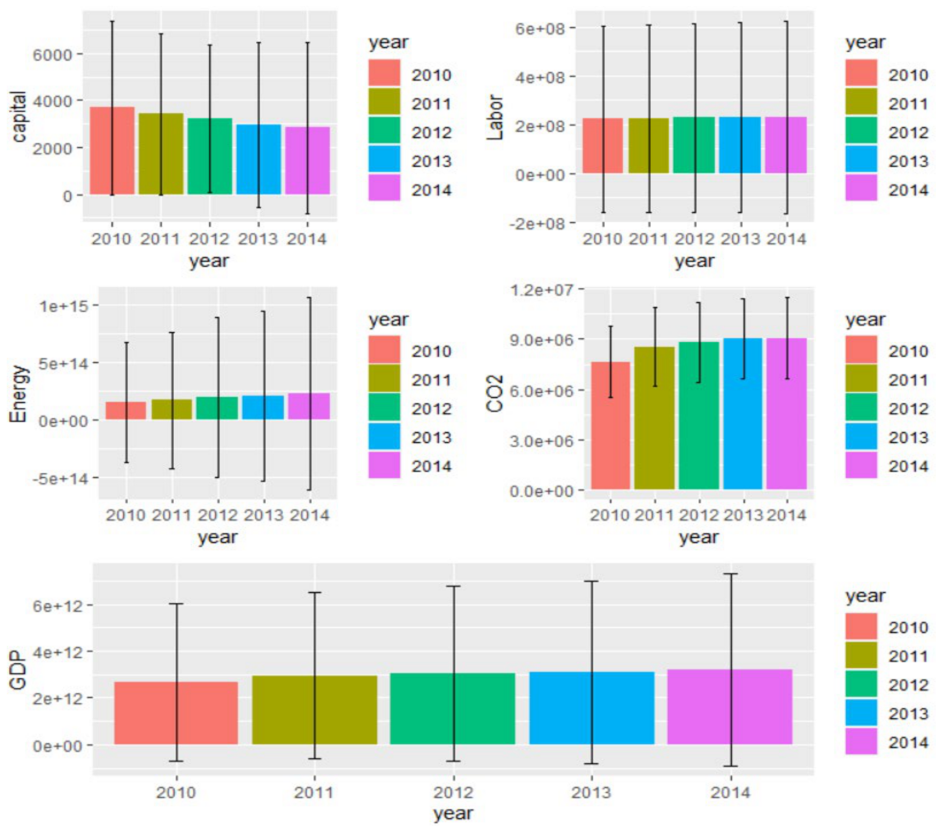
Before calculating the energy efficiencies of G20 economies, we provide a descriptive statistical analysis of the various indicators. The results are presented in Table 1 and Figure 1. Table 1 shows that the means of all indicators except for energy consumption increased from 2010 to 2014. The standard deviations of all indicators except for energy consumption also continued to increase over the five years, which illustrates that national differences in these indicators were expanding over this period. During these five years, China remained first in energy consumption and CO2 emissions, which is closely related to its long-standing coal-dominant energy system and its large population.
The empirical results for energy efficiency are presented in Table 2 and Figure 2 and Figure 3. The average energy efficiency of the G20 economies over the five years was 0.653. The energy efficiency of the G20 decreased annually from 0.6995 in 2010 to 0.5996 in 2014. The energy efficiency significantly differed across developed and developing economies in the G20. The five-year average efficiency of the nine developed economies in the G20 was 1.020, whereas the five-year average efficiency of the ten developing economies was only 0.323. The energy efficiency also varied significantly among the economies during the study period. Specifically, the economies with energy efficiencies above the average value of 0.653 were Argentina, Australia, Canada, France, Germany, Italy, the UK, and the USA, whereas the economies with efficiencies below the average value were Brazil, China, India, Indonesia, Japan, South Korea, Mexico, Russia, South Africa, Saudi Arabia, and Turkey. Among them, the economies with the top three five-year average efficiencies were the UK (1.701), the USA (1.606), and Australia (1.368), whereas the three economies with the lowest average efficiencies were China (0.006), India (0.061), and Indonesia (0.081).
Among the top three economies, the UK’s efficiency increased between 2010 and 2012 and began to decline in 2013. Both the USA and Australia remained relatively stable between 2010 and 2014, with efficiency values around 1.606 and 1.368, respectively. As for the bottom three economies, China performed poorly, with no significant improvement over the five years and a five-year average of only 0.006. The average efficiency of India between 2010 and 2014 was 0.061, with a continuous decreasing trend over the five years. Indonesia also performed poorly, with a five-year average of 0.081.
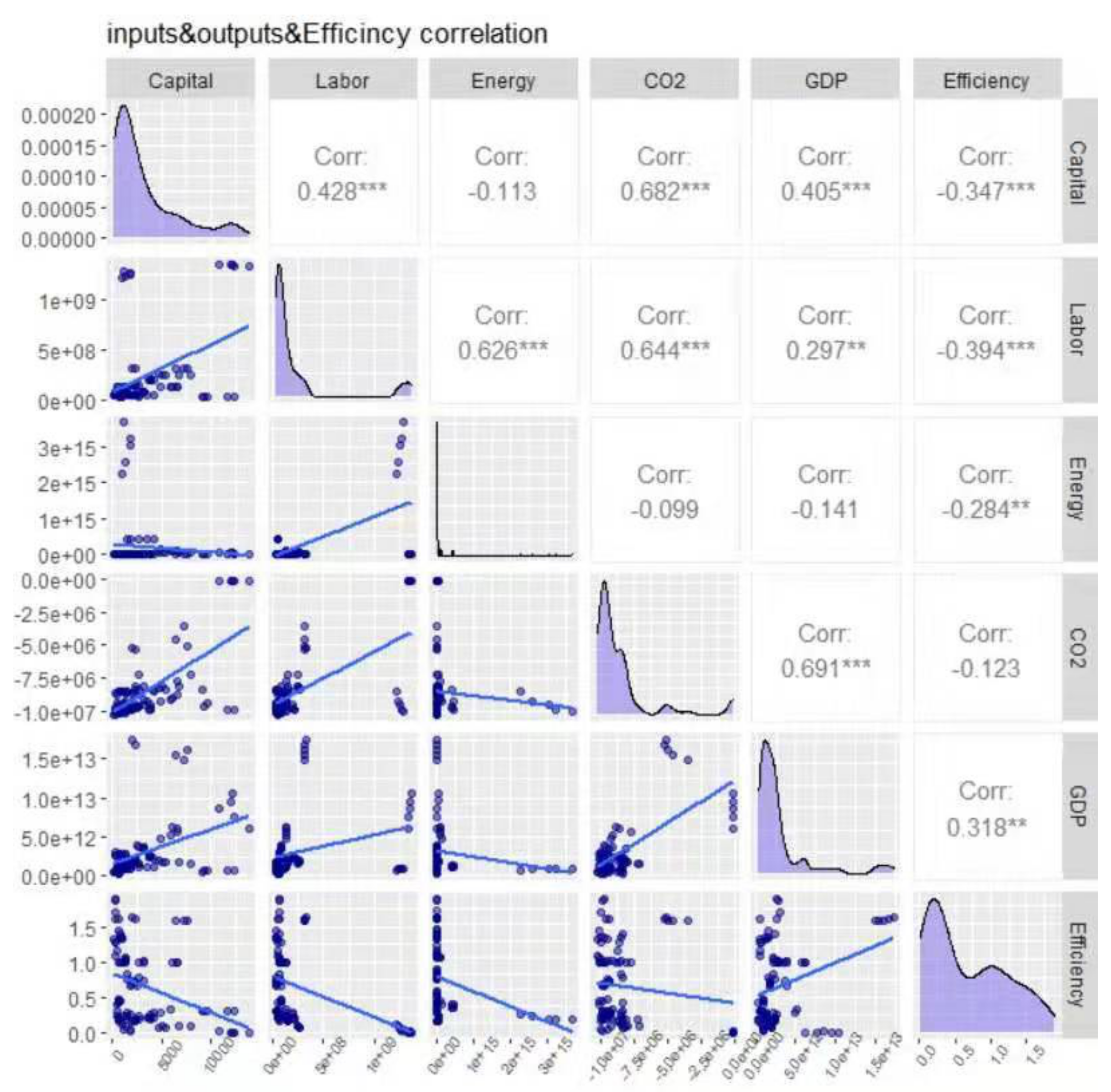
Then, we further analyzed which input variables and output variables have a significant impact on efficiency. Figure 4 shows that capital and labor have a negative impact on efficiency at the 1% confidence interval. At the 5% confidence interval, energy input has a negative impact on efficiency, and GDP has a positive impact on efficiency. According to the relationship between the above variables and the efficiency value, we can draw a conclusion that these four variables have a significant impact on the efficiency ranking.
4. Further Estimates of Energy Efficiency: Past-Present Model with Resampling
In the previous section, we used a triangular distribution to simulate the measurement error assuming that each DMU has an upper and a lower error rate. In this section, we used historical data for resampling purposes. The past-present model can improve the accuracy of estimates compared with the triangular model. The assumption of the past-present model is that the data variances differ across DMUs, and, thus, the estimation can be conducted using the historical data of each DMU.
Mehrotra and Sharma applied this method to assess the performance of multiple variables in a changing climate and proposed that changes in the dependence attributes can be ascertained by resampling the historical ranks into their potential future outcomes [37]. Their approach is not limited in terms of the number of variables, the number of grid points in space, and the time scale considered. In this study, we follow a similar methodology for all pairs of inputs, outputs, and inputs versus outputs in resampling, where inappropriate samples with unbalanced inputs and outputs are excluded from the resampling super-SBM DEA. This approach uses historical data to determine downside and upside error rates and utilizes the optimal weights of multiple periods of historical data to evaluate efficiency. The input and output variables are subject to change for several reasons, such as measurement error, hysteretic factors, and arbitrariness, under the DEA approach. Thus, DEA efficiency scores need to be examined by considering these factors. A resampling approach based on these variations is necessary to estimate the confidence intervals of the DEA scores. We also set the downside and upside error rate percentages to identify the reasons for poor efficiency across periods for all input and output data; this process is a very important contribution of this study. These results provide valuable references for the G20 economies in formulating policies for future energy use. This approach is suitable for researching energy use performance that may be affected by different periods.
The resulting 95% and 80% confidence intervals with resampling 1000 times are shown in Table 3 and Table 4. With 95% confidence intervals, no overestimated or underestimated cases arose. The average energy efficiency of the G20 was 0.8365, and the corrected efficiency value was 0.7834. The economies with efficiency values above the average value of 0.8365 were Argentina, Australia, France, Italy, the UK, and the USA, and the economies with efficiency values below the average value were Brazil, Canada, China, Germany, Indonesia, Japan, South Korea, Mexico, Russia, South Africa, and Turkey. The average efficiency of the nine developed economies in the G20 was 1.507 above the average value of 0.8365, whereas the average efficiency of the ten developing economies was only 0.233 below the average value. The corrected efficiency value of the nine developed economies in the G20 was 1.283 above the average value of 0.7834, whereas the corrected efficiency value of the ten developing economies was only 0.334 below the average value. Similarly, with 80% confidence intervals, no overestimated or underestimated cases arose. The average energy efficiency of the G20 was 0.8365, and the corrected efficiency value was 0.7834.
From the above analysis, although the G20 economies’ fossil fuel energy consumption continued to decrease between 2010 and 2014, GDP, the labor force, and capital stock continued to increase. However, the undesirable output of CO2 emissions also continued to increase, leading to a continuous decrease in energy efficiency (see Figure 2 and Figure 4). It seems that it will be difficult for the G20 economies to meet the CO2 reduction targets required by the Paris Agreement.
5. Conclusions and Policy Implications
Due to its high correlation with several key dimensions, including the economic, political, environmental, and social dimensions, energy governance has become one of the most important agendas in the current global governance process. In this study, we employed a triangular model to evaluate the energy efficiencies of the G20 economies from 2010 to 2014. Fossil fuel energy consumption, labor, and capital stock were taken as the input variables, and CO2 emissions and GDP were taken as the output variables. Additionally, a past-present model with resampling was used to measure whether the efficiency values of DMUs deviate for different confidence intervals. To the best of our knowledge, very few studies have applied the DEA method with resampling to analyze energy efficiency. Thus, our study contributes to the methodologies for energy efficiency evaluation.
Our study indicates that, based on the triangular model, the overall average energy efficiency of G20 economies from 2010 to 2014 was 0.653. The economies with the top three five-year average efficiencies were the UK (1.701), the USA (1.606), and Australia (1.368), whereas the three economies with the lowest average efficiencies were China (0.006), India (0.061), and Indonesia (0.081). The panel average efficiency of the developed countries was 1.020, higher than the overall average efficiency 0.653, and the panel average efficiency of the developing countries was 0.323, which is lower than the overall average efficiency 0.653. Energy efficiency also significantly differed across economies.
Using the past-present model with resampling to explore the error conditions, we found that the average energy efficiency of each DMU was 0.8365, the average adjustment value was 0.7834, and the average error value was 0.0531. The average efficiency of the nine developed economies in the G20 was 1.507, whereas the average efficiency of the ten developing economies was only 0.233. The corrected efficiency value of the nine developed economies in the G20 was 1.283 above the average value of 0.7834. whereas the corrected efficiency value of the ten developing economies was only 0.334. Under repeated sampling of the 95% and the 80% confidence intervals, we found no overestimation or underestimation of the results. We therefore conclude that under the past-present model with resampling, the acceptable error was 0.0531. Additionally, the top and bottom three economies in terms of energy efficiency were the same as in the triangular model.
The efficiency values estimated both by the triangular model and the past-present model with resampling showed that the developed countries performed better than the developing countries. The first point may be that the developing countries have a large population. In terms of transportation, construction, cooking, and industry, the demand for petrochemical energy is greater than that of developed countries. Therefore, energy consumption and CO2 emissions are far ahead of those of developed countries. The second point is that the energy technology and equipment (for example, clean energy) of developing countries are inferior to those of the developed countries. The third point is that, for the developing countries, the push for economic growth has largely ignored the environmental consequences. Our study proposed several recommendations. (1) To maintain the energy investment balance, the problem of inefficiency can be solved by correcting energy price distortions. (2) The habit of over-reliance on petrochemical energy should be converted to the use of renewable energy to achieve the goal of sustainable development. (3) The adoption of petrochemical energy subsidies by developing countries has resulted in an increase in energy consumption and worsening of the air. Renewable energy subsidies can be provided to developing countries through international green finance. In this way, the developing countries can improve energy efficiency and fulfill their responsibility to protect the environment while ensuring a stable electricity supply.
Our study innovatively employed the DEA method with resampling to analyze the energy efficiencies of G20 members. To confirm the reliability of our study’s results, further research can collect energy data from different economies around the world. Further studies can also focus on data collection starting in 2015 because, in 2015, each G20 economy submitted an expected proposal for future carbon reduction goals and strategies according to its national conditions to the United Nations Framework Convention on Climate Change. Thus, further studies should analyze whether each economy has achieved its promised emission reductions targets and whether energy efficiency has been improved in these economies.
In addition, although we use the resampling super-SBM DEA model to adjust the energy efficiency errors of G20 countries, in fact, some countries and their industries may cover the real results under the implementation of policies. In addition to the country’s commitment to reduce carbon emissions, nongovernment private actions and targets can also be conducive to achieving significant emissions reductions (Kuramochi et al., [38]; Lui et al., [39]; Mi et al., [40]). The estimated efficiency value may be underestimated. Therefore, the limitation of this study is that the participation of national policies will distort the national energy efficiency.
Author Contributions
Conceptualization, D.W.; data curation, C.-C.L. and P.-Y.T.; formal analysis, C.-C.L. and M.-L.W.; funding acquisition, D.W.; writing—original draft, D.W.; writing—review and editing, C.-C.L. and A.-C.Y. All authors have read and agreed to the published version of the manuscript.
Funding
This research was funded by the 312 Talent Training Project, Zhejiang Open University; Zhejiang Open University (RC050112211001); and the Academy of Financial Research, Zhejiang University.
Institutional Review Board Statement
Not applicable.
Informed Consent Statement
Not applicable.
Conflicts of Interest
The authors declare no conflict of interest.
References
- Sueyoshi, T.; Goto, M. Returns to scale and damages to scale with strong complementary slackness conditions in DEA assessment: Japanese corporate effort on environment protection. Energy Econ. 2012, 34, 1422–1434. [Google Scholar] [CrossRef]
- Hong, L.; Zhou, N.; Fridley, D.; Raczkowski, C. Assessment of China’s renewable energy contribution during the 12th Five Year Plan. Energy Policy 2013, 62, 1533–1543. [Google Scholar] [CrossRef]
- Song, M.L.; Zhang, L.L.; Liu, W.; Fisher, R. Bootstrap-DEA analysis of BRICS’ energy efficiency based on small sample data. Appl. Energy 2013, 112, 1049–1055. [Google Scholar] [CrossRef]
- Li, K.; Lin, B. Meta froniter energy efficiency with CO2 emissions and its convergence analysis for China. Energy Econ. 2015, 48, 230–241. [Google Scholar] [CrossRef]
- Chiu, Y.H.; Shyu, M.K.; Lee, J.H.; Lu, C.C. Undesirable output in efficiency and productivity: Example of the G20 countries. Energy Sources Part B Econ. Plan. Policy 2016, 11, 237–243. [Google Scholar] [CrossRef]
- Guo, X.; Lu, C.C.; Lee, J.H.; Chiu, Y.H. Applying the dynamic DEA model to evaluate the energy efficiency of OECD countries and China. Energy 2017, 134, 392–399. [Google Scholar] [CrossRef]
- Fernández, D.; Pozo, C.; Folgado, R.; Jiménez, L.; Guillén-Gosálbez, G. Productivity and energy efficiency assessment of existing industrial gases facilities via data envelopment analysis and the Malmquist index. Appl. Energy 2018, 212, 1563–1577. [Google Scholar] [CrossRef]
- Antonietti, R.; Fontini, F. Does energy price affect energy efficiency? Cross-country panel evidence. Energy Policy 2019, 129, 896–906. [Google Scholar] [CrossRef]
- Qi, S.; Peng, H.; Zhang, X.; Tan, X. Is energy efficiency of Belt and Road Initiative countries catching up or falling behind? Evidence from a panel quantile regression approach. Appl. Energy 2019, 253, 113581. [Google Scholar] [CrossRef]
- Farrell, M.J. The measurement of productive efficiency. J. R. Stat. Soc. 1957, 120, 253–281. [Google Scholar] [CrossRef]
- Charnes, A.; Cooper, W.W.; Rhodes, E. Measuring the efficiency of decision making units. Eur. J. Oper. Res. 1978, 2, 429–444. [Google Scholar] [CrossRef]
- Banker, R.D.; Charnes, A.; Cooper, W.W. Some models for estimating technical and scale inefficiencies in data envelopment analysis. Manag. Sci. 1984, 30, 1078–1092. [Google Scholar] [CrossRef] [Green Version]
- Hsieh, J.C.; Ma, L.H.; Chiu, Y.H. Assessing China’s Use Efficiency of Water Resources from the Resampling Super Data Envelopment Analysis Approach. Water 2019, 11, 1069. [Google Scholar] [CrossRef] [Green Version]
- Tone, K.A. Slacks-based measure of efficiency in data envelopment analysis. Eur. J. Oper. Res. 2001, 130, 498–509. [Google Scholar] [CrossRef] [Green Version]
- Tone, K.A. Slacks-based measure of super-efficiency in data envelopment analysis. Eur. J. Oper. Res. 2002, 143, 32–41. [Google Scholar] [CrossRef] [Green Version]
- Tone, K.; Quenniche, J. DEA scores’ confidence intervals with past-present and past-present-future based resampling. Am. J. Oper. Res. 2016, 6, 121–135. [Google Scholar] [CrossRef] [Green Version]
- Simar, L.; Wilson, P.W. Sensitivity analysis of efficiency scores: How to bootstrap in nonparametric frontier models. Manag. Sci. 1998, 44, 49–61. [Google Scholar] [CrossRef] [Green Version]
- Simar, L.; Wilson, P.W. A general methodology for bootstrapping in non-parametric frontier models. J. Appl. Stat. 2000, 27, 779–802. [Google Scholar] [CrossRef]
- Tone, K. Resampling in DEA; National Graduate Institute for Policy Studies: Tokyo, Japan, 2013. [Google Scholar]
- Fang, H.H.; Lee, H.S.; Hwang, S.N.; Chung, C.C. A slacks-based measure of super-efficiency in data envelopment analysis: An alternative approach. Omega 2013, 41, 731–734. [Google Scholar] [CrossRef]
- Arabi, B.; Munisamy, S.; Emrouznejad, A. A new slacks-based measure of Malmquist–Luenberger index in the presence of undesirable outputs. Omega 2015, 51, 29–37. [Google Scholar] [CrossRef] [Green Version]
- Lozano, S.; Gutiérrez, E. Slacks-based measure of efficiency of airports with airplanes delays as undesirable outputs. Comput. Oper. Res. 2011, 38, 131–139. [Google Scholar] [CrossRef]
- Chiu, Y.H.; Chen, Y.C.; Bai, X.J. Efficiency and risk in Taiwan banking: SBM super-DEA estimation. Appl. Econ. 2011, 43, 587–602. [Google Scholar] [CrossRef]
- Li, H.; Shi, J. Energy efficiency analysis on Chinese industrial sectors: An improved Super-SBM model with undesirable outputs. J. Clean. Prod. 2014, 65, 97–107. [Google Scholar] [CrossRef]
- Du, H.; Matisoff, D.C.; Wang, Y.; Liu, X. Understanding drivers of energy efficiency changes in China. Appl. Energy 2016, 184, 1196–1206. [Google Scholar] [CrossRef]
- Zhang, J.; Zeng, W.; Wang, J.; Yang, F.; Jiang, H. Regional low-carbon economy efficiency in China: Analysis based on the Super-SBM model with CO2 emissions. J. Clean. Prod. 2017, 163, 202–211. [Google Scholar] [CrossRef]
- Zhou, C.; Shi, C.; Wang, S.; Zhang, G. Estimation of eco-efficiency and its influencing factors in Guangdong province based on Super-SBM and panel regression models. Ecol. Indic. 2018, 86, 67–80. [Google Scholar] [CrossRef]
- Li, Y.; Chiu, Y.H.; Lu, L.C.; Chiu, C.R. Evaluation of energy efficiency and air pollutant emissions in Chinese provinces. Energy Effic. 2019, 12, 963–977. [Google Scholar] [CrossRef]
- Bai, X.; Zeng, J.; Chiu, Y.H. Pre-evaluating efficiency gains from potential mergers and acquisitions based on the resampling DEA approach: Evidence from China’s railway sector. Transp. Policy 2019, 76, 46–56. [Google Scholar] [CrossRef]
- Luo, G.; Wang, X.; Wang, L.; Guo, Y. The Relationship between Environmental Regulations and Green Economic Efficiency: A Study Based on the Provinces in China. Int. J. Environ. Res. Public Health 2021, 18, 889. [Google Scholar] [CrossRef]
- Lo Storto, C. Performance evaluation of social service provision in Italian major municipalities using Network Data Envelopment Analysis. Socio-Econ. Plan. Sci. 2020, 71, 100821. [Google Scholar] [CrossRef]
- Ma, L.-H.; Hsieh, J.-C.; Chiu, Y.-H. A study of business performance and risk in Taiwan’s financial institutions through resampling data envelopment analysis. Appl. Econ. Lett. 2020, 27, 886–891. [Google Scholar] [CrossRef]
- Chang, T.-S.; Tone, K.; Wu, C.-H. Past-present-future Intertemporal DEA models. J. Oper. Res. Soc. 2015, 66, 16–32. [Google Scholar] [CrossRef]
- Lo Storto, C. A double-DEA framework to support decision-making in the choice of advanced manufacturing technologies. Manag. Decis. 2018, 56, 488–507. [Google Scholar] [CrossRef]
- Färe, R.; Grosskopf, S.; Lovell, C.A. Kand Pasurka, C. Multilateral Productivity Comparisons When Some Outputs are Undesirable: A Nonparametric Approach. Rev. Econ. Stat. 1989, 71, 90–98. [Google Scholar] [CrossRef]
- Seiford, L.M.; Zhu, J. Modeling undesirable factors in efficiency evaluation. Eur. J. Oper. Res. 2002, 142, 16–20. [Google Scholar] [CrossRef]
- Mehrotra, R.; Shrama, A. A Resampling Approach for Correcting Systematic Spatiotemporal Biases for Multiple Variables in a Changing Climate. Water Resour. Res. 2019, 55, 754–770. [Google Scholar] [CrossRef] [Green Version]
- Kuramochi, T.; den Elzen, M.; Peters, G.P.; Bergh, C.; Crippa, M.; Geiges, A.; Godinho, C.; Gonzales-Zuñiga, S.; Hutfilter, U.F.; Keramidas, K.; et al. Global emissions trends and G20 status and outlook—Emissions gap report Chapter 2. In Emissions Gap Report; UNEP: Nairobi, Kenya, 2020; pp. 3–22. [Google Scholar]
- Lui, S.; Kuramochi, T.; Smit, S.; Roelfsema, M.; Hsu, A.; Weinfurter, A.; Chan, S.; Hale, T.; Fekete, H.; Lütkehermöller, K.; et al. Correcting course: How international cooperative initiatives can build on national action to steer the climate back towards Paris temperature goals. Clim. Policy 2020, 21, 232–250. [Google Scholar] [CrossRef]
- Mi, Z.; Guan, D.; Liu, Z.; Liu, J.; Viguié, V.; Fromer, N.; Wang, Y. Cities: The core of climate change mitigation. J. Clean. Prod. 2019, 207, 582–589. [Google Scholar] [CrossRef]
Figure 1.
Descriptive statistics of input and output from 2010 to 2014.

Figure 2.
Comparison of CROSS AVE between developed countries and developing countries.
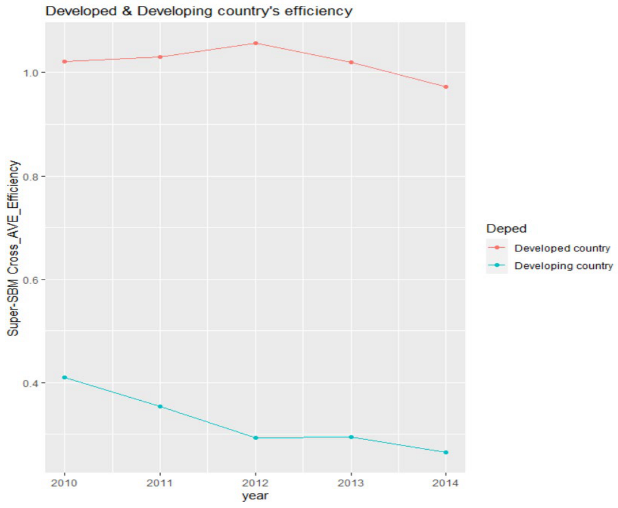
Figure 3.
Five-year average energy efficiencies.
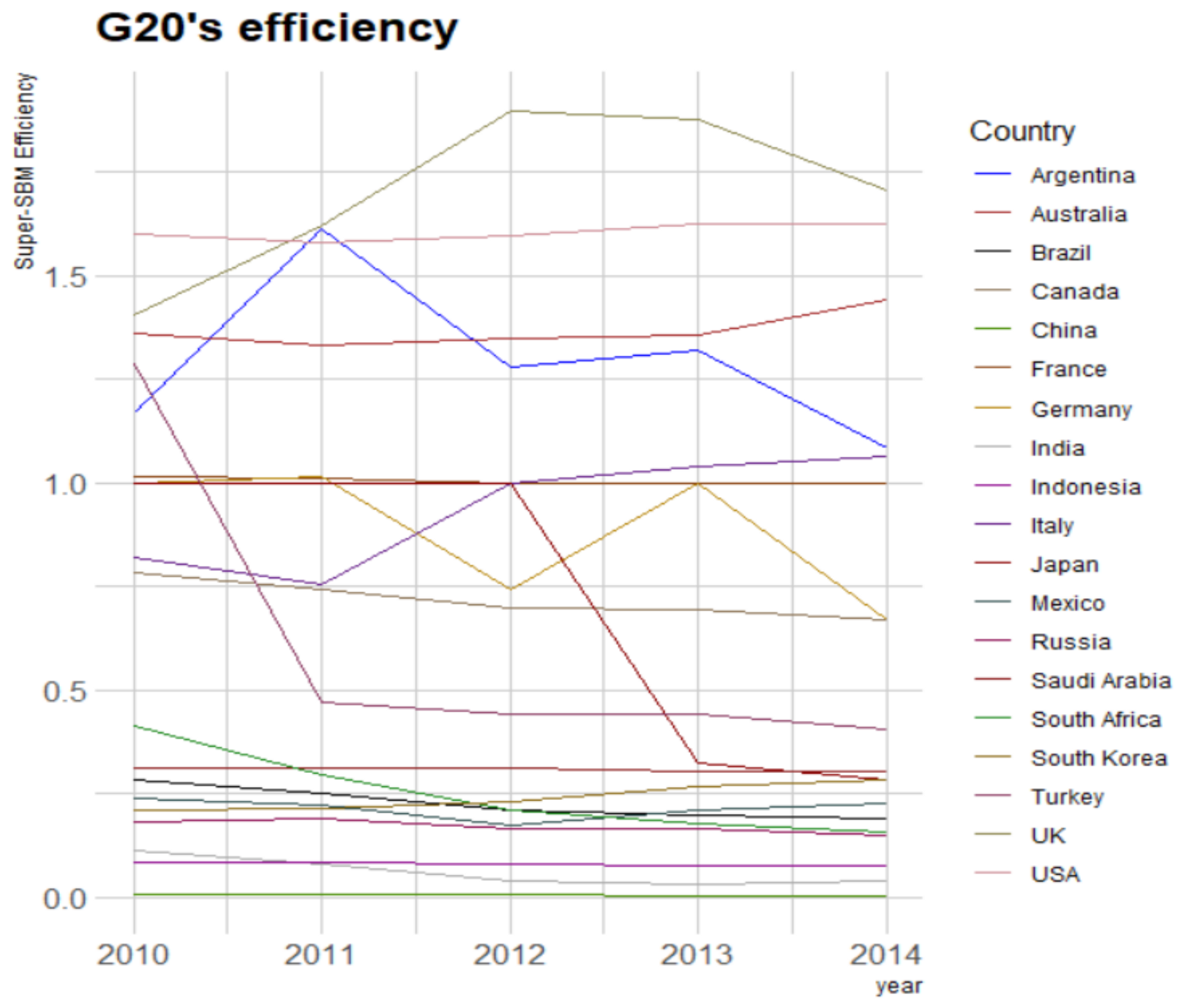
Figure 4.
Correlation coefficient between input, output, and efficiency.


Table 1.
Descriptive statistical analysis of various indicators.
| Year | Indicator | Capital Stock | Labor | Energy Consumption | CO2 | GDP |
|---|---|---|---|---|---|---|
| (Million Dollars) | (Kilotons) | (Million Dollars) | ||||
| 2010 | Mean | 149,478,189 | 108,316,017 | 3692.56 | 7,646,724.5 | 2,660,091 |
| Standard deviation | 505,038,661 | 186,929,215 | 3607.73 | 2,094,422.84 | 3,294,967 | |
| Maximum | 2,256,935,300 | 779,956,733 | 13,931.6 | 8,776,040.4 | 14,964,372 | |
| Minimum | 247,717 | 9,834,264 | 285 | 187,919.08 | 375,298 | |
| 2011 | Mean | 169,230,754 | 108,814,101 | 3410.5254 | 8,543,152.14 | 2,955,362 |
| Standard deviation | 577,458,420 | 187,495,914 | 3335.3605 | 2,265,896.44 | 3,473,192 | |
| Maximum | 2,583,242,604 | 783,018,630 | 12,419.9829 | 9,733,538.12 | 15,517,926 | |
| Minimum | 254,402 | 10,487,696 | 231 | 191,633.753 | 416,878 | |
| 2012 | Mean | 192,298,266 | 109,598,429 | 3216.8684 | 8,811,079.76 | 3,032,865 |
| Standard deviation | 673,764,086 | 187,953,077 | 3075.9077 | 2,308,862.99 | 3,660,775 | |
| Maximum | 3,021,664,869 | 785,504,321 | 10,907.5 | 10,028,573.9 | 16,155,255 | |
| Minimum | 265,549 | 11,202,506 | 249 | 192,356.152 | 396,333 | |
| 2013 | Mean | 203,087,907 | 110,539,620 | 2,958 | 9,034,164.41 | 3,106,234 |
| Standard deviation | 719,496,298 | 189,008,990 | 3396.7 | 2,360,714.98 | 3,803,718 | |
| Maximum | 3,229,586,653 | 787,010,207 | 11,948 | 10,258,007.1 | 16,691,517 | |
| Minimum | 272,062 | 11,845,700 | 182 | 189,851.591 | 366,810 | |
| 2014 | Mean | 227,358,805 | 111,457,383 | 2828.4632 | 9,071,316.71 | 3,190,252 |
| Standard deviation | 814,347,761 | 190,020,711 | 3534.57 | 2,378,675.01 | 4,010,851 | |
| Maximum | 3,657,154,385 | 788,179,264 | 12,403 | 10,291,926.9 | 17,393,103 | |
| Minimum | 276,246 | 12,339,232 | 246 | 204,024.546 | 351,119 |
Source: Compiled by public data of the World Bank (https://data.worldbank.org.cn/, and https://cdiac.ess-dive.lbl.gov/trends/emis/top2014.tot (accessed on 29 June 2021)), United Nations database (UNDATA).
Table 2.
Energy efficiencies of G20 economies.
| Economies | 2010 | 2011 | 2012 | 2013 | 2014 | Time_AVE |
|---|---|---|---|---|---|---|
| Australia | 1.3596 | 1.3315 | 1.3476 | 1.3559 | 1.443 | 1.368 |
| Canada | 0.7836 | 0.7447 | 0.6979 | 0.6957 | 0.6689 | 0.718 |
| France | 1.0148 | 1.0108 | 0.9997 | 0.9997 | 0.9997 | 1.005 |
| Germany | 0.9992 | 1.0173 | 0.7451 | 0.9995 | 0.6701 | 0.886 |
| Italy | 0.822 | 0.7545 | 0.9996 | 1.0405 | 1.0641 | 0.936 |
| Japan | 0.9999 | 0.9999 | 0.9999 | 0.3254 | 0.285 | 0.722 |
| South Korea | 0.2125 | 0.2139 | 0.2294 | 0.2688 | 0.2843 | 0.242 |
| UK | 1.4052 | 1.6203 | 1.8975 | 1.8763 | 1.7056 | 1.701 |
| USA | 1.6008 | 1.5784 | 1.598 | 1.6246 | 1.6263 | 1.606 |
| Developed country Cross AVE | 1.022 | 1.030 | 1.057 | 1.021 | 0.972 | 1.020 |
| Argentina | 1.1697 | 1.6128 | 1.2784 | 1.3183 | 1.0865 | 1.293 |
| Brazil | 0.2844 | 0.2504 | 0.211 | 0.2001 | 0.1922 | 0.228 |
| China | 0.0059 | 0.0065 | 0.0082 | 0.005 | 0.0053 | 0.006 |
| India | 0.1127 | 0.0813 | 0.039 | 0.0314 | 0.0411 | 0.061 |
| Indonesia | 0.0841 | 0.0833 | 0.0818 | 0.0775 | 0.0772 | 0.081 |
| Mexico | 0.2396 | 0.2239 | 0.1758 | 0.2129 | 0.2255 | 0.216 |
| Russia | 0.1822 | 0.191 | 0.1674 | 0.1667 | 0.1517 | 0.172 |
| South Africa | 0.4139 | 0.2977 | 0.2116 | 0.1795 | 0.1575 | 0.252 |
| Saudi Arabia | 0.3119 | 0.3128 | 0.311 | 0.3047 | 0.3034 | 0.309 |
| Turkey | 1.2894 | 0.4726 | 0.442 | 0.4437 | 0.4044 | 0.610 |
| Developing country Cross AVE | 0.409 | 0.353 | 0.293 | 0.294 | 0.265 | 0.323 |
| Cross_AVE | 0.700 | 0.674 | 0.655 | 0.638 | 0.600 | 0.653 |
Notes: The economies in this table are developed countries (Australia, Canada, France, Germany, Italy, Japan, South Korea, UK, USA) outlined in yellow, and developing countries (Argentina, Brazil, China, India, Indonesia, Mexico, Russia, South Africa, Saudi Arabia, Turkey) outlined in blue.
Table 3.
Efficiency values and 95% confidence intervals for G20 economies.
| DMU | Efficiency Value | Corrected Efficiency Value | Deviation | Lower Bound (2.5%) | Upper Bound (97.5%) |
|---|---|---|---|---|---|
| Australia | 1.3959 | 1.4105 | −0.0146 | 1.2956 | 1.5265 |
| Canada | 0.6589 | 0.7792 | −0.1203 | 0.5960 | 1.0515 |
| France | 0.9996 | 0.8707 | 0.1289 | 0.5011 | 1.1120 |
| Germany | 0.6393 | 0.8573 | −0.2180 | 0.5484 | 1.0711 |
| Italy | 1.1235 | 1.0556 | 0.0679 | 0.5986 | 1.1687 |
| Japan | 0.2543 | 0.4064 | −0.1521 | 0.2488 | 0.9999 |
| South Korea | 0.3327 | 0.3635 | −0.0308 | 0.1959 | 0.9997 |
| UK | 6.4996 | 4.1660 | 2.3336 | 1.1959 | 11.0024 |
| USA | 1.6593 | 1.6374 | 0.0219 | 1.5623 | 1.7072 |
| Developed country Cross AVE | 1.507 | 1.283 | 0.224 | 0.749 | 2.293 |
| Argentina | 1.0740 | 1.1669 | −0.0929 | 0.3359 | 1.6533 |
| Brazil | 0.1711 | 0.2576 | −0.0865 | 0.1584 | 0.9996 |
| China | 0.0044 | 0.0055 | −0.0011 | 0.0027 | 0.0112 |
| India | 0.0099 | 0.0455 | −0.0356 | 0.0092 | 0.1225 |
| Indonesia | 0.0653 | 0.0741 | −0.0088 | 0.0600 | 0.0976 |
| Mexico | 0.1400 | 0.3776 | −0.2376 | 0.1196 | 1.0700 |
| Russia | 0.1324 | 0.1516 | −0.0192 | 0.1163 | 0.2058 |
| South Africa | 0.1271 | 0.3063 | −0.1792 | 0.1270 | 0.9994 |
| Saudi Arabia | 0.3004 | 0.4752 | −0.1748 | 0.2457 | 0.9999 |
| Turkey | 0.3050 | 0.4768 | −0.1718 | 0.2022 | 0.9998 |
| Developing country Cross AVE | 0.233 | 0.334 | −0.101 | 0.138 | 0.716 |
| Cross_AVE | 0.8365 | 0.7834 | 0.0531 | 0.4273 | 1.4631 |
Notes: The economies in this table are developed countries (Australia, Canada, France, Germany, Italy, Japan, South Korea, UK, USA) outlined in yellow, and developing countries (Argentina, Brazil, China, India, Indonesia, Mexico, Russia, South Africa, Saudi Arabia, Turkey) outlined in blue.
Table 4.
Efficiency values and 80% confidence intervals for G20 economies.
| DMU | Efficiency Value | Corrected Efficiency Value | Deviation | Lower Bound (10%) | Upper Bound (90%) |
|---|---|---|---|---|---|
| Australia | 1.3959 | 1.4105 | −0.0146 | 1.3333 | 1.4851 |
| Canada | 0.6589 | 0.7792 | −0.1203 | 0.6262 | 1.0224 |
| France | 0.9996 | 0.8707 | 0.1289 | 0.542 | 1.0416 |
| Germany | 0.6393 | 0.8573 | −0.218 | 0.5954 | 1.048 |
| Italy | 1.1235 | 1.0556 | 0.0679 | 0.9998 | 1.1337 |
| Japan | 0.2543 | 0.4064 | −0.1521 | 0.2592 | 0.9995 |
| South Korea | 0.3327 | 0.3635 | −0.0308 | 0.2271 | 0.4785 |
| UK | 6.4996 | 4.166 | 2.3336 | 1.3696 | 7.9619 |
| USA | 1.6593 | 1.6374 | 0.0219 | 1.5841 | 1.6914 |
| Developed country Cross AVE | 1.507 | 1.283 | 0.224 | 0.837 | 1.874 |
| Argentina | 1.074 | 1.1669 | −0.0929 | 1.0366 | 1.3685 |
| Brazil | 0.1711 | 0.2576 | −0.0865 | 0.1686 | 0.2969 |
| China | 0.0044 | 0.0055 | −0.0011 | 0.0034 | 0.0086 |
| India | 0.0099 | 0.0455 | −0.0356 | 0.0099 | 0.0833 |
| Indonesia | 0.0653 | 0.0741 | −0.0088 | 0.0626 | 0.0873 |
| Mexico | 0.14 | 0.3776 | −0.2376 | 0.1285 | 0.9998 |
| Russia | 0.1324 | 0.1516 | −0.0192 | 0.1226 | 0.1841 |
| South Africa | 0.1271 | 0.3063 | −0.1792 | 0.1395 | 0.9957 |
| Saudi Arabia | 0.3004 | 0.4752 | −0.1748 | 0.2745 | 0.9996 |
| Turkey | 0.305 | 0.4768 | −0.1718 | 0.231 | 0.9996 |
| Developing country Cross AVE | 0.233 | 0.334 | −0.101 | 0.218 | 0.602 |
| Cross_AVE | 0.8365 | 0.7834 | 0.0531 | 0.5113 | 1.2045 |
Notes: The economies in this table are developed countries (Australia, Canada, France, Germany, Italy, Japan, South Korea, UK, USA) outlined in yellow, and developing countries (Argentina, Brazil, China, India, Indonesia, Mexico, Russia, South Africa, Saudi Arabia, Turkey) outlined in blue.
Publisher’s Note: MDPI stays neutral with regard to jurisdictional claims in published maps and institutional affiliations. |
© 2021 by the authors. Licensee MDPI, Basel, Switzerland. This article is an open access article distributed under the terms and conditions of the Creative Commons Attribution (CC BY) license (https://creativecommons.org/licenses/by/4.0/).
Share and Cite
MDPI and ACS Style
Wu, D.; Lu, C.-C.; Tang, P.-Y.; Wang, M.-L.; Yang, A.-C. A Resampling Slack-Based Energy Efficiency Analysis: Application in the G20 Economies. Energies 2022, 15, 67. https://doi.org/10.3390/en15010067
AMA Style
Wu D, Lu C-C, Tang P-Y, Wang M-L, Yang A-C. A Resampling Slack-Based Energy Efficiency Analysis: Application in the G20 Economies. Energies. 2022; 15(1):67. https://doi.org/10.3390/en15010067
Chicago/Turabian StyleWu, Dan, Ching-Cheng Lu, Pao-Yu Tang, Miao-Ling Wang, and An-Chi Yang. 2022. "A Resampling Slack-Based Energy Efficiency Analysis: Application in the G20 Economies" Energies 15, no. 1: 67. https://doi.org/10.3390/en15010067
Note that from the first issue of 2016, this journal uses article numbers instead of page numbers. See further details here.