
A Calibration of the Solar Load Ratio Method to Determine the Heat Gain in PV-Trombe Walls


Mechanical, Energy and Management Engineering Department, University of Calabria, P. Bucci 46/C, Arcavacata di, 87036 Rende, CS, Italy
*
Author to whom correspondence should be addressed.
Energies 2022, 15(1), 328; https://doi.org/10.3390/en15010328
Submission received: 1 December 2021
/
Revised: 17 December 2021
/
Accepted: 1 January 2022
/
Published: 4 January 2022
(This article belongs to the Special Issue High-Efficiency Thermal-Storage Devices and Systems)
Abstract
:The Trombe wall is a passive system used in buildings that indirectly transfers thermal energy to the adjacent environment by radiation and convection, and directly by the thermo-circulation that arises in the air cavity delimited between a transparent and an absorbing surface. Nevertheless, the latter is painted black to increase the energy gains, but this produces a negative visual impact and promotes the overheating risk in summer. To mitigate these aspects, a hybrid Trombe wall equipped with PV panels can be employed. The PV installation results in a more pleasing wall appearance and the overheating risk reduces because part of the absorbed solar radiation is transformed into electricity. To determine the actual performance of a such system, transient simulation tools are required to consider properly the wall thermal storage features, variation of the optical properties, air thermo-circulation, and PV power production. Alternatively, regarding the traditional Trombe wall, the literature provides a simplified empirical method based on the dimensionless parameter solar load ratio (SLR) that allows for preliminary evaluations and design. In this paper, the SLR method was calibrated to determine the monthly auxiliary energy to be supplied in buildings equipped with PV-Trombe walls in heating applications. The SLR method was tuned by a multiple linear regression by data provided by TRNSYS simulation that allowed to obtain the energy performances in actual conditions of PV-Trombe walls installed on the same building but located in different localities. The comparison between the TRNSYS results and the calibrated SLR method determined average errors ranging between 0.7% and 1.4%, demonstrating the validity of the proposed methodology.
1. Introduction
The energy availability allows for the development and the benefit growth for society, by promoting the improvement of life quality [1]. Nevertheless, the current lifestyle is still too distracted towards the energy consumption issues and, often, it is in contrast to the current energy situation [2]. In this regard, the research activities look toward production systems based on renewable sources and to develop targeted strategies for limiting energy wastes [3,4]. These systems are more appreciated when integrated into the building sector in which a lot of energy is often dispersed [5,6]. Indeed, edifices are responsible for 40% of the global energy consumption for final uses and 36% of the CO2 emission, with the sole residential sector that contributes by 25.4% of the total demand [7]. Suitable legislative plans have been developed to improve energy efficiency politics, as well as energy savings interventions and integration of renewable sources in the building sector [8,9,10]. In light of this, the application of a passive system is attractive because these allow for attaining energy savings exploiting solar radiation as the primary energy source, without the use of mechanical devices to move a heat transfer fluid [11,12]. The Trombe–Michel wall is a relevant example classified as an indirect heat gain system, in which solar energy is collected and stored in the same element. Successively, it is employed by convection, radiation, and thermo-circulation to heat an adjacent indoor environment [13,14].
One negative aspect of a Trombe wall is related to the evident visual impact connected with the black-painted exterior surface. To alleviate these issues, recently designers have looked at the PV-Trombe wall with great interest [15,16]. The installation of a PV generator allows for attaining a more pleasing appearance. Furthermore, the conversion of part of the incident solar radiation in electric energy allows for limiting the absorption of the thermal energy in the massive wall by reducing the overheating risk. By considering that in the air-gap elevated temperatures can be achieved, the application of PV panels with thin-film cells appears more appropriate because this technology is less affected by the thermal drift effect [17]. Additionally, these cells can benefit from the colored anti-reflective glass or directly integrated with the glass cover (semi-transparent covers), whereas, when installed on the massive wall, the limited thickness allows for conferring a reduced thermal resistance without interfering negatively with the transmitted thermal flux. Last but not least, these cells are cheaper than crystalline technology.
Currently, PV panels can be installed in different parts of the Trombe walls: some experimental setups include PV cells inside the glass cover (PVTW-G), on the massive wall (PVTW-M), and sometimes on the shading blinds (PVTW-B). In [18], a comparative study between a PV-Trombe wall and a traditional Trombe wall, both equipped with Venetian blinds installed in the air-gap for shading and air-flow regulation purposes, was carried out in a semi-arid region of Saudi Arabia, numerically and experimentally. Considering the particular climate, it was proven that PV cells integrated with the glass cover (PVTW-G) produced a massive wall temperature decrement down to 5.2 °C and a correspondent decrement of the heat gain of about 33%, confirming the goodness of such choice to contrast the indoor overheating. Generally, as stated in [19] by a proper model validated by measured data under the Hefei warm climatic context (China), the cover ratio growth on the glass produced an increase of the PV production and the total efficiency of the PV-Trombe wall. Moreover, a decrement in the indoor temperature and the thermal efficiency was observed. Nevertheless, semi-transparent covers integrating PV cells have to be evaluated carefully to avoid a worsening of the winter thermal performances in severe climatic conditions. In order to investigate the impact of the PV cells in the external cover, in [20] a comparison among different typologies of Trombe walls employing a single pane, a double pane, and a-Si cell integrated into a single pane, was carried out under the climatic conditions of Izmir (Turkey) by an experimental test room. The authors stated that PV cells allow for producing a noticeable reduction of the temperature inside the air-gap, again a worsening of the thermal performances was observed in winter, whereas the installation of the double-pane covers improve the heat gains. The thermal performances of particular configurations of PV-Trombe walls with a semi-transparent cover were studied in [21] including a windowed surface on the south façade to determine the winter temperature field inside the heated room. The authors proved that the design of the south façade affects the PV-Trombe wall efficiency noticeably, in particular, thermal efficiency could decrease up to 27%, whereas the PV coverage growth determined a reduction of thermal gains up to 17%. Similar work was conducted in [22] by adding a supplementary heat storage system in a fenestrated room, which allowed attaining an increase of the indoor air temperature up to 7.7 °C. Meanwhile, the daily average electric efficiency was 10.4%. In order to quantify the effects of PV glass instead of a traditional cover, the model developed in [23] determined a maximum difference of 12.3 °C in the indoor air temperature in free-floating conditions. To facilitate the identification of a suitable compromise between winter and summer performances, the employment of forced ventilation in the air-gap by DC fans, instead of natural ventilation, was considered. A double-layer Trombe wall not equipped with PV panels but assisted by a DC fan was investigated in [24], and results proved a thermal performances improvement of 5.6%. Regarding the comparison between the results of a PVTW-G equipped with a DC fan with a traditional installation, in [25] it was determined that in winter the forced ventilation allows for an average indoor temperature increase of 0.5 °C. Simultaneously, the PV cells temperature decreased on average of 1.28 °C with a correspondent improvement of the electric efficiency. Alternatively, to avoid the penalization of the winter heat gain, PV cells can be integrated also into appropriate blinds installed in the air-gap (PVTW-B), as studied in [26]. The authors found that an airflow rate of 0.45 m/s with a blind tilt angle of 50° is recommended, because in this configuration, by combining heat gains and electric power, the system efficiency was superior by 14.5% and 14.1% than PVTW-G and PVTW-M, respectively. In particular, the comparative study carried out in [27] concerning these Trombe wall typologies in the warm climate of Hefei highlighted an annual electric output of PVTW-B similar to those of PVTW-G, when the blind angles are changed during the year to optimize the incident solar radiation. Moreover, more than 20% of the electric energy than the PVTW-M was produced. Another way to avoid the limitation of solar gains in winter is the installation of PV panels in the middle of the air-gap (built-middle PV-Trombe wall), as investigated in [28]. The total efficiency of a such system was 10.83% superior to that achievable in a traditional PVTW-G. Moreover, an optimal distance between PV modules and glass cover was identified in 12–30 mm to maximize total, thermal, and electric efficiencies. A way to improve the electric performances of PV modules in PVTW-M configurations, penalized by the thermal drift effect, was investigated in [29] in which authors proposed the employment of a mixture of water and nanoparticles as coolant circulating in a heat exchanger installed behind the PV panels.
In general, the literature highlights that the employment of PVTW-G is recommended in warm climates due to their capability to modulate the absorption of the solar radiation in the massive wall, limiting the overheating risk. However, a significant increment of the heating requirement can be detected in continental climates due to the penalization of the heat gains. Furthermore, the literature provides few documents related to the actual performance of PVTW-M. In particular, procedures to quantify how the PV cells interfere with the thermal heat gains, necessary in design evaluation and for building energy certification purposes, have not been found. In light of this, the aim of this work is the evaluation of a simple method to determine the performance of a PVTW-M equipped with PV cells to use for preliminary design assessments. Considering the electric power as an extra output, attention is paid to the precise evaluation of the heat gain to use for the reduction of the heating demand, which represents the main target in a Trombe wall installation. In this regard, the SLR (solar load ratio) steady-state method, indicating the ratio between the employed solar energy and the thermal demand required from the building, is very attractive due to its simplicity, employing a correlation based on three constants. For PVTW-M configurations, however, these constants are not available; therefore, the present document aims to update the SLR method by analyzing data obtained from TRNSYS dynamic simulation [30]. To consider the actual performance in terms of achieved heat gains, a reference building equipped with different solutions of PVTW-M located in different localities with appreciable heating demands was simulated. The PVTW-M configuration does not limit the heat gain excessively as detected in PVTW-G installations, promoting rational exploitation of the solar source. The interaction of detailed TRNSYS models concerning the building [31], the Trombe wall, and the PV generator has allowed the actual performance of the system to be determined in detail, by taking into account the effects connected with the storage features of the Trombe wall, the variation of the optical properties of the glass cover with the directional aspects of the solar radiation, the airflow rate generated in the air-gap, and the thermal drift of the PV cells. The analysis of such data, by multiple linear regressions, has allowed the new values of the aforementioned constants to be determined in order to implement the SLR method also for PVTW-M walls. In the following, the paper describes the Trombe wall working and the SLR method by the correspondent analytical procedure. Successively, the case study analyzed by TRNSYS was described and the correspondent results used for the multiple non-linear regression targeted to extend the SLR method in PV-Trombe walls in which the active solar system is installed on the massive surface.
2. Materials and Methods
2.1. Trombe Wall Operation
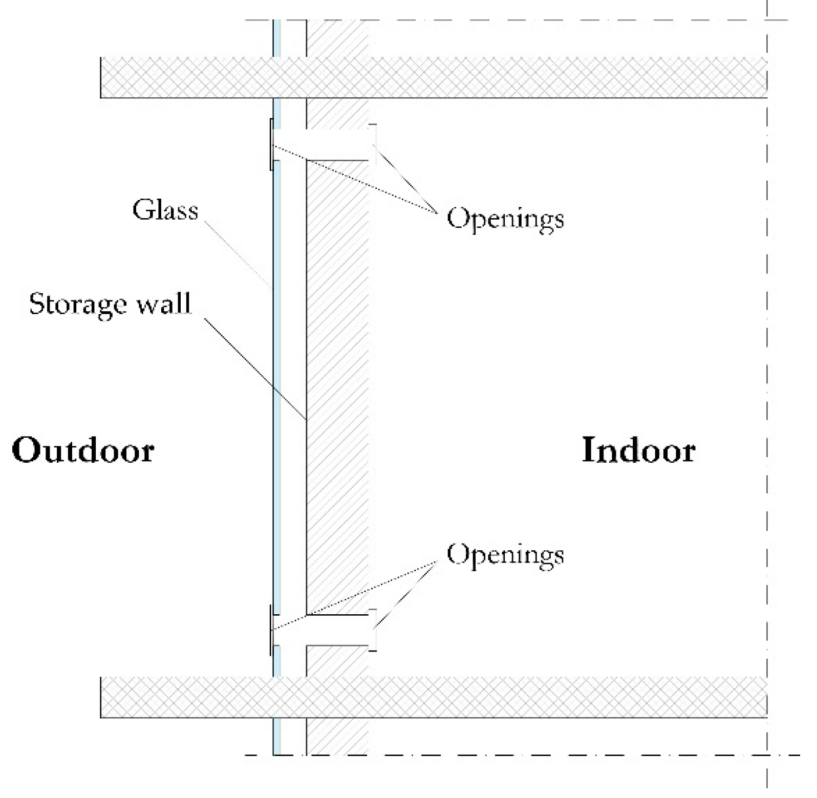
The Trombe wall was proposed for the first time in 1967 and it consists of a massive south-facing wall whose external surface is painted black to facilitate solar radiation absorption. Moreover, the high thermal inertia allows for exploiting the stored thermal energy also at night. One or more transparent covers allow for separating the absorbing surface from the external environment to limit thermal losses [32], forming an air gap in which the thermo-circulation occurs (see Figure 1). The transparent surface is equipped with an overhang opportunely sized to create shading in summer. Moreover, suitable blinds obscure the absorption surface during the summer days, or are activated at night in winter to reduce the thermal losses. Both massive walls and transparent surfaces are equipped with proper openings (vents) that allow for rational exploitation of the airflow rate produced by the natural convection.
On sunny winter days, the wall vents are opened, while the glass vents are closed to promote natural convection in the indoor environment, whereas at night the wall vents are closed to avoid an inverse air circulation. Nevertheless, the indoor environment can still be heated by exploiting the heat stored in the massive wall. On summer days the vents on the transparent surface are opened, leaving closed those on the massive wall, promoting the cooling of the absorbing surface to discharge the thermal energy stored in the wall. At night, instead, the opening of the vents allows transferring internal thermal loads outward by natural ventilation (see Figure 2) [13].
It is worth noting that the Trombe wall modifies the internal mean radiant temperature, and in combination with the velocity of the air exiting the massive wall vents, could produce a worsening of the indoor thermal comfort conditions. Thus, suitable control strategies deciding the opening/closing of the vents have to be evaluated carefully to find the best compromise with the energy savings [33,34]. In this regard, different investigations have been carried out to determine the appropriate management of the Trombe wall as a function of the climatic contexts both in winter and summer [35,36]. Alternatively, structural modifications were proposed to optimize the performances [37,38,39].
2.2. The SLR Method
The SLR method was developed by Balcomb [40] and it is generalizable for every passive system installed in buildings. The Balcomb theory, derived from experimental analysis, uses the SLR concept calculated by a series of empirical correlations to determine the SSF (solar saving fraction), namely the share of the heating demand covered by the solar source, by a correlation employing three constant values that currently are listed in proper tables, but only for traditional Trombe walls. This procedure was validated exclusively for the winter period, and it is targeted to quantify the actual heat gain provided by the passive system to reduce the heating energy demand. In buildings with passive systems, the SLR approach allows for determining at a monthly level the thermal energy that the solar source (Esol) can make available to cover a part of the net building thermal requirement (Enet), namely the energy requirement determined for the building without considering thermal losses through the same passive system. It is defined as a solar saving fraction (SSF) and it can be calculated by the relation:
showing that this share depends on two constants (C and D as a function of the passive system features) and the solar load ratio (SLR), the latter defined as the ratio between the monthly solar energy absorbed from the building and its monthly net thermal heating demand. SLR is determined with the following relation:
in which another constant (H) appears. The SLR depends on the load collector ratio (LCR, ) that represents the global thermal losses, again calculated excluding the Trombe wall, and assuming a unitary temperature difference between indoor and outdoor air, and successively normalized to the passive system surface. SLR depends also on LCRS that, instead, represents the global thermal losses between the air-gap and the external environment, again normalized to the surface of the transparent cover () and depends on the external cover features. LCR can be determined by using the relationship described in Equation (5) diving it by the Trombe wall surface, while in Equation (2) S represents the monthly solar energy absorbed in the massive wall (in kWh/m2 per month) and normalized by the number of heating degree-day (DD). The latter is a climatic index related to the locality and it can be determined with the formula:
where Toa is the daily average outdoor air temperature determined on the jth day of the month (with N days), whereas Tb is the reference indoor set-point temperature corrected by taking into account daily endogenous energies (Qend, in for appliances, people, artificial lighting, and similar). It has to be noticed that in the summation, only the differences that provide a positive value have to be considered. When the winter set-point is set to 20 °C, Tb is determined as:
in which TLC (total loss coefficient) is used to quantify the total thermal losses (transmission and ventilation) through the building envelope per a unitary temperature difference between internal and external air temperature. TLC is related to the average transmission loss coefficient of the building envelope determined on a global dispersing surface Atot (conversely to LCR, this time also the surface of the Trombe wall must be involved). The average coefficient is calculated by a weighted mean of every U-value concerning the surface of the dispersing element. Furthermore, TLC depends on the mean ventilation loss coefficient determined by multiplication of the ventilation flow rate and the air volumetric thermal capacity (about 1200 J/m3K):
Regarding the net monthly thermal energy demand of the building (determined by excluding the thermal losses through the passive system) it can be determined easily as:
in which NLC (net load coefficient, in ) is the daily thermal losses of the building per unity of temperature difference between indoor and outdoor determined without considering the Trombe wall, and it can be employed also for the LCR calculation.
2.3. Investigated Case Study
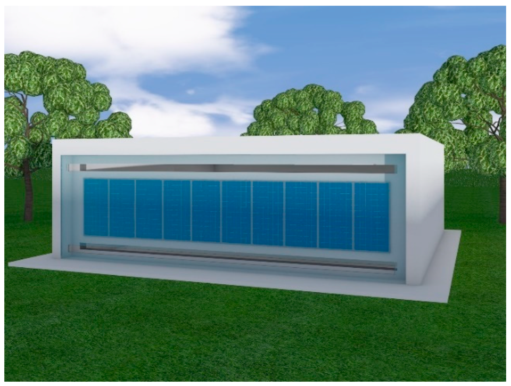
The dynamic simulations carried out by TRNSYS involved the reference single-storey building depicted in Figure 3 with a gross dimension of 10 × 10 × 3 m and a net heated surface of about 60 m2. The south façade is entirely occupied by the Trombe wall with 23.25 m2 of net surface, whereas other windowed surfaces are located at north and west. The vertical opaque walls are all well-insulated with a thermal transmittance of 0.23 W/m2K. An insulated flat roof and a dispersing ground floor with U-values of 0.25 W/m2K complete the thermal zone, whose indoor air was maintained at a constant set-point temperature of 20 °C. For the evaluation of the monthly thermal energy demands, endogenous gains of 330 W and natural ventilation of 0.5 air-change per hour was set in the simulations.
To obtain a sufficient number of data required to perform the multiple regression to determine the new constant values by fitting Equations (1) and (2), the same reference building was located in three different climatic zones. These latter are characterized by the different availability of solar radiation. Nevertheless, these have in common a significant number of heating degree-days (HDD), ranging between 2200 and 2500, which allow determining appreciable heating demands (Table 1). The latter, at a seasonal level, is equal to 1506, 1841, and 1852 kWh, respectively, for the locality A, B, and C, assuming an adiabatic south wall. To obtain a more general correlation, different configurations of the Trombe wall were simulated, varying the thermal properties of the massive wall and the number of external covers, as described in Table 2 [41]. Such configurations, however, do not consider the presence of the PV cells, because their physical properties do not affect the Trombe wall features in an evident manner.
2.4. The Procedure to Determine the SLR Constants for PVTW-M Configurations
The thermal energy balance of a PV-Trombe wall can be expressed by the following equation:
where S is the energy absorbed in the massive wall, EG,I is the thermal energy transferred by the massive wall, EL,S are the thermal losses toward the air-gap, Eel is the electric energy rate, and is the variation of internal energy.
Simulation performed by TRNSYS allowed for determining every term appearing in Equation (7). To determine the absorbed energy in the massive wall (S), a constant solar absorbing coefficient (αs) of 0.95 was set, whereas, to determine the actual share striking the massive wall, the product solar transmittance-absorption of the external cover was varied dynamically as a function of the incident angle (i) of the beam solar radiation, by the relation [42]:
in which the constant b0 and the optical properties for normal incidence are set to 0.10 and 0.80 for external covers with a single pane, 0.17 and 0.70 with a double pane, and 0.22 and 0.65 with a triple pane. The transmittance of diffuse and reflected solar radiation is computed at an equivalent angle of incidence of 60°. The thermal energy (EG,i) transferred by the massive wall was determined by quantifying the convection and the infrared radiation shares toward the indoor environment. The internal convective heat transfer was set constant to 3.05 W/m2K [43], whereas the radiative one was determined internally by TRNSYS as a function of the enclosure features. The thermal losses toward the air-gap were determined with a constant longwave emission coefficient (εl) of 0.9 for the wall and 0.837 for the glass and by considering a coolant airflow rate driven by the temperature difference between the mean temperature in the air-gap and the room temperature. The air-flow rate was calculated internally in the model by setting 6% of the vent surface of the massive wall area with a vertical distance of 2.65 m. Finally, the electric energy rate (Eel) was determined by assuming thin-film PV technology whose peak power is 2.15 kW (21 m2) with the electric characteristics listed in Table 3. In simulations, a coupled direct electric load was considered, and the performances were determined as a function of an empirical equivalent circuit model to predict the current-voltage characteristics and the power output. The procedure employed at a monthly level to determine the new SLR constant values for every PV-Trombe wall listed in Table 2 follows these steps:
- The building net monthly thermal energy demand Enet was determined by TRNSYS with an indoor air set-point temperature of 20 °C. In order to deduct the thermal losses through the analyzed Trombe wall, following the SLR method, an initial building configuration was simulated without a Trombe wall but with an adiabatic surface south facing, as well as LCR was calculated maintaining the same envelope properties;
- SLR was varied by changing location and the Trombe wall configurations that determined different LCRS values. In particular, the latter was obtained as an output of the Trombe wall model by setting a pane thickness of 4 mm and, for multiple covers, an air-cavity of 14 mm with air-filled. In a simplified way, the thermal losses toward outdoor were determined with a constant combined heat transfer coefficient l of 25 W/m2K, following the procedures for the building energy certification [44]. LCR, instead, remained constant being the thermal properties of the simulated building the same across the considered localities;
- The heat gain Esol was quantified by summing convective and radiative contributes from the Trombe wall inner surface and the thermal load provided by the air-flow crossing the vents;
- Monthly SSFs were determined by dividing the prior two energy contributions;
- S is a further output of the TRNSYS model, whereas DD was determined analytically by the daily outdoor air temperature detected in every locality using Equations (3) and (4). Again, Qend is provided by TRNSYS whereas TLC was calculated in parallel simulations in which the hypothesis of adiabatic south wall was removed;
- A linear multiple regression analysis was carried out to calculate the new values of C, D, and H.
3. Results
Since the Balcomb method was developed starting from experimental data, initially the comparison of the SSF values was carried out by the simulations results involving traditional Trombe walls. Indeed, the simulated walls are identical; however, Balcomb obtained its results starting from different localities and with other building configurations. Therefore, unavoidable deviances are expected. The data listed in Table 4, related to the performances provided by the Trombe wall TWA3 and TWD2 in the three considered climatic contexts, showed that an appreciable match was anyway detected. These walls were chosen because they have the same physical properties but a different number of external covers. TRNSYS simulations tended to underestimate the SSF, with differences that increase with the latitude growth and, for the same location, decrease with the Trombe wall performances. It can be noticed that the TWD2 solution allows for attaining higher SSF due to a major limitation of the air-gap thermal losses. Results showed a maximum and acceptable discrepancy of 6% detected for the colder localities and in the coldest period of the year, both for TWA3 and TWD2. It is worth noting that the SSF trends follow the outdoor air temperature and solar radiation availability trend quite well, meaning that the passive system performances are prevalently affected by the augment of the building heating demand and the offered heat gain. Indeed, it has to be noticed that in locality C, the maximum deviances of 6% was observed in December both for TWA3 and TWD2 due to the lowest values of outdoor temperature and incident solar radiation.
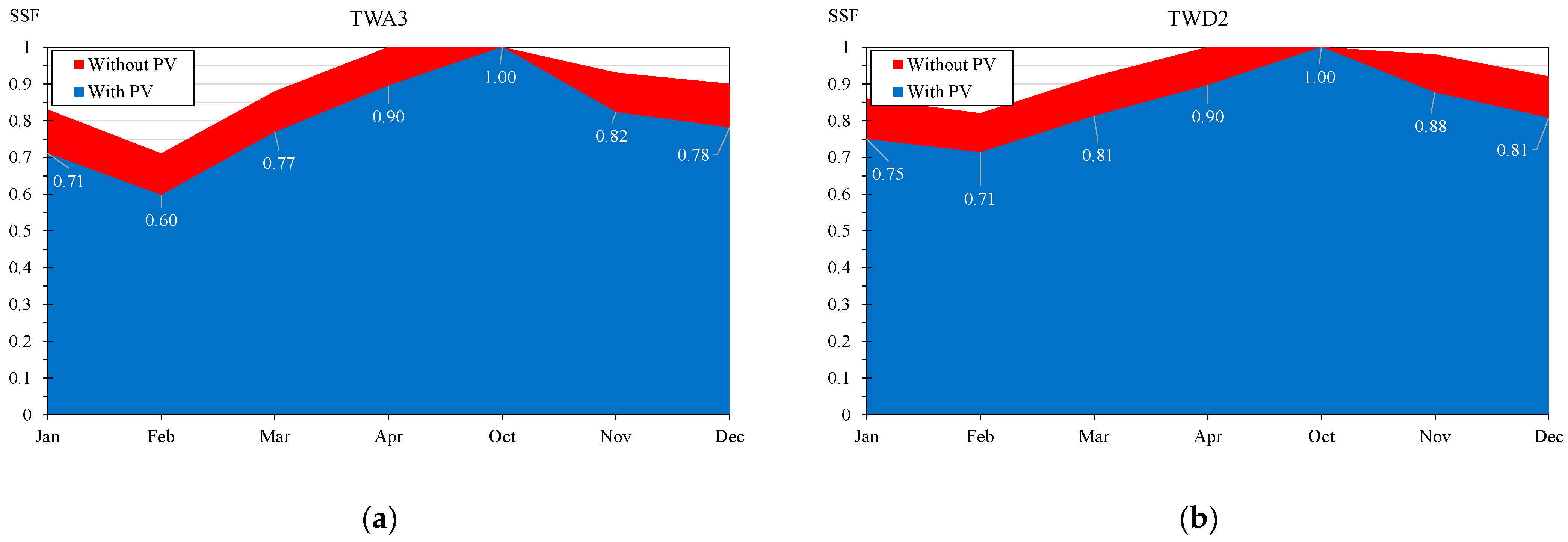
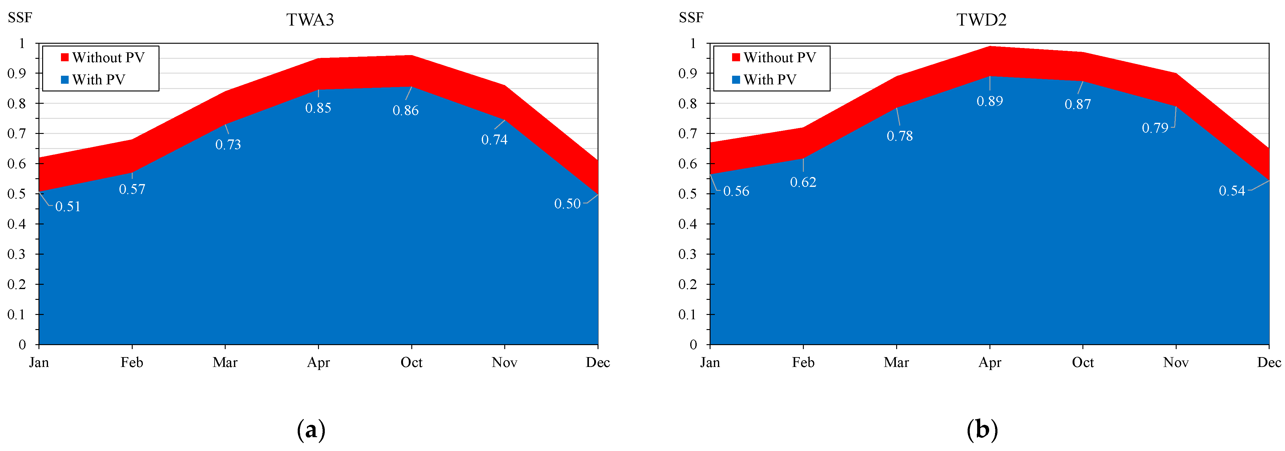
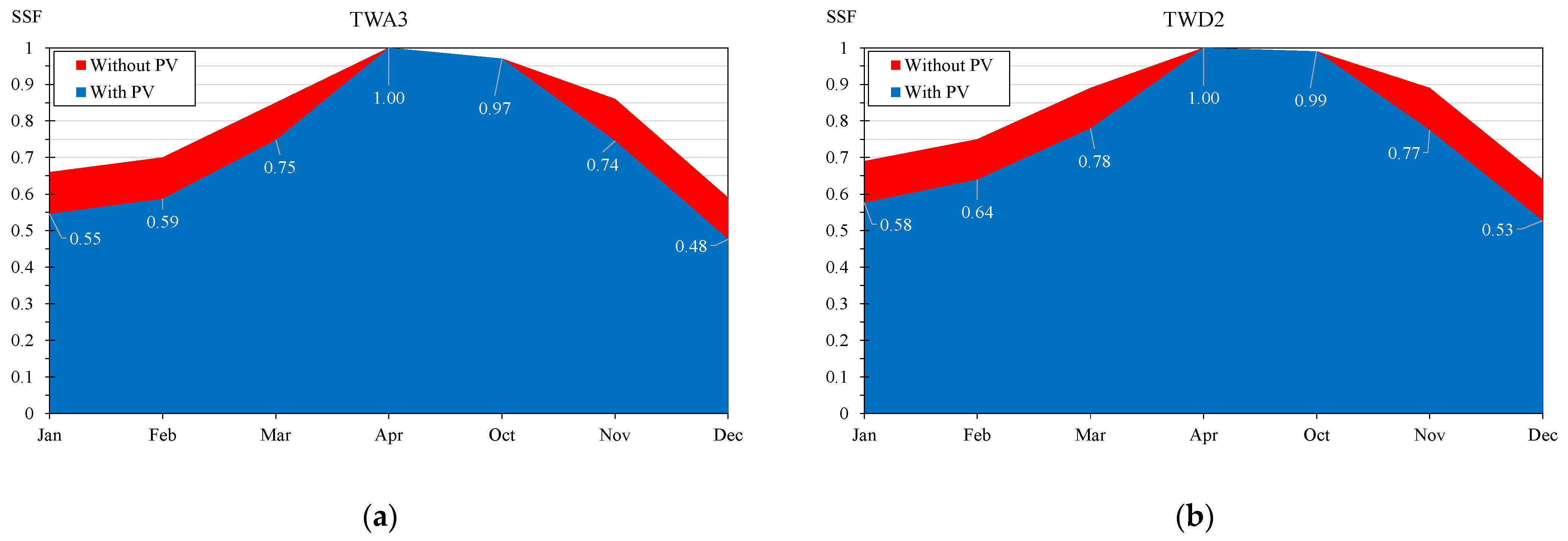
In Figure 4, Figure 5 and Figure 6, for every considered locality, the SSFs determined by TRNSYS for the TWA3 and TWD2 configurations, with and without PV generators, are shown. It is worth noting that the SSFs of the investigated PVTW-M decrease due to the limitation of the heat gains, and the differences tend to change slightly among the monthly belonging to the heating period. Furthermore, it can be appreciated that the deviances between the SSF determined in traditional and PV-Trombe walls is more or less coincident with the monthly electric efficiency of the PV panels. Regarding the first locality (Figure 4), it can be noticed that the SSFs coincide in October due to the reduced magnitude of the heating requirement, therefore the produced heat gain, despite the production of the renewable electricity, is still enough to satisfy the energy demand completely. In the other months, instead, SSFs decrease by about ten percentage points, with maximum deviance of 11.96% in December and a minimum difference of 10.49% in April. The SSF decrements remain almost constant during the heating period, because electric efficiency changes slightly; however, the gap tends to reduce limitedly at the beginning and the end of the heating period. Regarding the second configuration of the Trombe wall, the SSF deviances trend is similar; however, in absolute terms, the differences are minor than the prior case because of the lower production of the PV generator. Indeed, the TWD2 configuration produces about 750 kWh/kWp during the heating period instead of 791 kWh/kWp detected for the TWA3 solution: this is due to the different number of external covers that, in the first case, produces a slight decrement in the incident solar radiation on the PV panels. Nevertheless, the heat gain is not affected negatively, because the limitation of the thermal losses counterbalances the minor availability of solar radiation.
In the second locality (Figure 5), with a more severe winter climate, the differences in SSF remain almost constant during the heating period, with maximum and minimum deviations equal, respectively, to 11.55% (November) and 10.48% (October) for the TWA3 solution. For the other one, again, the difference was reduced in the interval 9.67–11.04%, due to the lower PV production of 582 instead of 620 kWh/kWp.
Similar trends and deviations have been observed in Figure 6 for locality C. Again, it is confirmed that in the months with reduced heating energy demands the limitation of the heat gain is not penalizing for the SSF.
By using the results of TRNSYS simulations to determine the values of SLR and SSF analytically, the values of the constants appearing in Equations (1) and (2) have been determined by fitting the data with the least-squares method, obtaining for the PVTW-M configuration the new values listed in Table 5. Moreover, the same table shows the data to use in traditional Trombe wall, to have a term of comparison.
From a preliminary analysis, it can be noticed that the constant H in PVTW-M configurations is subjected to little variation, and it is mainly affected by the air-gap thermal losses as confirmed by the TWE2 configuration equipped with a low-ε glass. The limited variation of the constant H could be justified by the unchangeable LCR values; this assumption is acceptable considering that the tendency is to design a well-insulated building to comply with the constraints in terms of energy consumptions containment. More appreciable variations have been detected both for the C and the D constant. In particular, targeted investigations have shown the dependency of the latter from the nominal efficiency of the PV panel. Finally, due to the lack of sufficient data with a limited value of SLR provided by simulations, the employment of the data listed in Table 5 is recommended when SLR is greater than 0.15. When the SLR method was implemented in PVTW-M with the constant values listed in Table 5, and by applying optical properties averaged monthly to determine the share of solar radiation incident on the PV surface, the comparison conducted with the TRNSYS results has provided an average error ranging between 0.7% and 1.4%, whereas the worst value determined for the RMSE amounted to 6.3%, confirming that the calibrated method allows for attaining reliable SSFs also for the specific configuration of Trombe wall with PV panel on the massive surface.
Application of the Calibrated SLR Method to the Reference Building: Simplified Procedure
Excluding the Trombe wall, the building depicted in Figure 3 is characterized by average transmission and ventilation heat loss coefficients equal respectively to 68.08 W/m2 °C and 23.74 W/m2K, for a total value of 91.82 W/m2 °C, and a correspondent NLC of 2.204 kWh/°C per day. When the south-facing wall is involved in the calculation, the global loss coefficient increases to 104.47 W/m2K, with a correspondent TLC value of 2.507 kWh/°C per day. In light of this, with the assumed internal gains (7.92 kWh per day), the reference temperature Tb is 16.8 °C; therefore, when the building is placed in the locality A, the heating degree-day listed in Table 6 can be calculated. Because the surface of the passive system is 23.25 m2, LCR is 0.095 kWh/(m2 °C) per day and, with the hypothesis to install the TWA2 configuration, an external cover thermal transmittance of 2.8 W/m2 °C can be associated, with a correspondent LCRS value of 0.0672 kWh/(m2 °C) per day. Regarding the absorbed solar radiation share, it can be calculated by Equation (8) by employing the monthly average daily values of the incidence angles () of the beam component [45], assuming instead a constant value of 0.9 for the absorbing surface. Thus, the SLR, and successively the SSF values, can be determined for a traditional Trombe wall and a PVTW-M configuration, with results shown in Table 6.
The results highlight that, between the two Trombe wall configurations, deviances of about 10% can be observed in the coldest period, whereas in the warm months the percentage differences are less pronounced because the heat gain gap is anyway counterbalanced by a correspondent decrement of the heating requirements. The latter is a methodology to verify the thermal performance provided by a PVTW-M imposing a precise collection surface; however, the same methodology can be extended also to preliminary design evaluations. For instance, it is possible to determine the required Trombe wall surface to supply in the coldest month (February) almost an SSF of 50%. Thus, the SLR can be derived by the inverse solution of Equation (1), obtaining 1.045 and 1.434, respectively, for a traditional and a PVTW-M configuration. Successively, making explicit the surface of the passive system in Equation (2) by LCR, it is possible to determine a value of 15.3 m2 in the first case and an increased value of 20.8 m2 in the second one. This result confirms that, in every case, the reduction of the heat gain due to the PV installation could be counterbalanced by an increase of the collection surface and, in the specific worst case, this augment is about 36%.
4. Conclusions
The employment of PV Trombe walls is even more considered by designers to alleviate two critical issues of such passive system: the first aesthetic, due to external black painted surface, the second one related to the comfort conditions due to the overheating risk in presence of elevated solar irradiation. Nevertheless, the installation of PV panels on the massive surface of a Trombe wall leads to a limitation of the heat gain for the adjacent environment; therefore, the implementation of simplified procedures targeted to determine how the attained Solar Saving Fraction (SSF) is affected by the active solar system, is appreciated. In light of this, in this paper, a calibration of the steady SLR procedure developed by Balcomb to determine the energy performance of traditional Trombe walls was conducted to apply the same approach also for PV Trombe walls. The results provided by dynamic simulations carried out in the TRNSYS environment have allowed for considering the interaction of passive and active solar systems in detail, and these data were used in a multiple non-linear regression to find new values of the constants involved in the SLR procedure. The comparison of the results provided by the SLR method between a traditional Trombe wall and an analogous configuration equipped with a PV generator allowed for determining that, on average, the heat gain is negatively affected of a percentage similar to the nominal PV efficiency, by exclusively in the coldest months. Furthermore, air-gap thermal losses remain almost the same being the attained temperature levels similar, therefore the PV installation does not interfere negatively with the air thermo-circulation heat gain. The limited thickness and the favorable thermal properties of the PV thin-film cells, instead, do not influence the storage properties of the massive wall. During the warmer period, the SLR is less penalized because the reduction of the heat gains benefits of a correspondent limitation of the heating demands. Nevertheless, the limitation of the heat gain due to the PV installation can be easily recovered by a precise collection surface growth. The comparison conducted with the TRNSYS results confirmed the reliability of the calibration procedure in light of an average error ranging between 0.7% and 1.4% and the highest RMSE of 6.3% determined among different Trombe wall configurations. The calibration procedure, due to the lack of pertinent data in the multiple non-linear regression, is limited to SLR values that have to be greater than 0.15. The developed procedure allows for determining in a simplified manner the actual performance of the PV Trombe wall when the collection surface is set, to use these results also for building certification purposes. Alternatively, the same approach can be used for design evaluations to determine the surface of the passive system necessary to achieve a precise SSF value. It has to be noticed that, at a seasonal level, the installation of the PV generator in the three considered localities produced an increase of the thermal energy requirement that is of the same order of magnitude of the electric energy produced by the PV generators. Therefore, the employment of electric heat pump systems supplied by the same renewably electricity allows for producing additional thermal energy. Finally, concerning the traditional approach, of the three constants that appear in the SLR method, one is subjected to slight variation because it is strongly dependent on the envelope features, whereas the other two constants show a sort of dependence on the nominal efficiency of the PV cells. Future investigation in this direction will be performed to identify suitable correlations to correlate these two constants to the PV cell’s electric efficiency.
Author Contributions
Conceptualization, R.B., P.B., D.C. and S.P.; Methodology, R.B., D.C., S.P. and A.R.; Investigation, R.B., P.B., D.C., S.P. and A.R.; Supervision, R.B.; Writing—Original Draft Preparation, R.B.; Formal analysis, P.B.; Software, P.B., P.B., D.C., S.P. and A.R. All authors have read and agreed to the published version of the manuscript.
Funding
This research received no external funding.
Conflicts of Interest
The authors declare no conflict of interest.
References
- Liu, B.; Matsushima, J. Annual changes in energy quality and quality of life: A cross-national study of 29 OECD and 37 non-OECD countries. Energy Rep. 2019, 5, 1354–1364. [Google Scholar] [CrossRef]
- Bogin, D.; Kissinger, M.; Erell, E. Comparison of domestic lifestyle energy consumption clustering approaches. Energy Build. 2021, 253, 111537. [Google Scholar] [CrossRef]
- Adedoyin, F.F.; Bekun, F.V.; Alola, A.A. Growth impact of transition from non-renewable to renewable energy in the EU: The role of research and development expenditure. Renew. Energy 2020, 159, 1139–1145. [Google Scholar] [CrossRef]
- Paoletti, G.; Pascuas, R.P.; Pernetti, R.; Lollini, R. Nearly Zero Energy Buildings: An Overview of the Main Construction Features across Europe. Buildings 2017, 7, 43. [Google Scholar] [CrossRef]
- Schregle, R.; Renken, C.; Wittkopf, S. Spatio-Temporal Visualisation of Reflections from Building Integrated Photovoltaics. Buildings 2018, 8, 101. [Google Scholar] [CrossRef] [Green Version]
- Shushunova, T.; Shushunova, N.; Pervova, E.; Dernov, R.; Nazarova, K. Tendencies of the green construction in Russia. In Proceedings of the IOP Conference Series: Materials Science and Engineering, Prague, Czech Republic, 15–19 June 2020. [Google Scholar]
- European Parliament. Directive 2012/27/EU of the European Parliament and of the Council on Energy Efficiency; Official Journal of the European Union, European Union: Brussels, Belgium, 2012. [Google Scholar]
- European Commission. Directive (EU) 2018/844 of the European Parliament and of the Council of 30 May 2018 Amending Directive 2010/31/EU on the Energy Performance of Buildings and Directive 2012/27/EU on Energy Efficiency; European Commission: Brussels, Belgium, 2018; Volume 156, pp. 1–17. [Google Scholar]
- Shushunova, N.S.; Korol, E.A.; Vatin, N.I. Modular Green Roofs for the Sustainability of the Built Environment: The Installation Process. Sustainability 2021, 13, 13749. [Google Scholar] [CrossRef]
- Korol, E.; Shushunova, N.; Nikitina, M.; Shushunova, T. Modular greening technologies for buildings. E3S Web Conf. 2021, 263, 04031. [Google Scholar] [CrossRef]
- Bruno, R.; Arcuri, N.; Carpino, C. The passive house in Mediterranean area: Parametric analysis and dynamic simulation of the thermal behavior of an innovative prototype. Energy Procedia 2015, 82, 533–539. [Google Scholar] [CrossRef] [Green Version]
- Nemś, M.; Kasperski, J. A Set-up for an Experimental Verification of a New Conception of Solar Powered House. Energy Procedia 2014, 57, 2305–2314. [Google Scholar] [CrossRef] [Green Version]
- Hu, Z.; He, W.; Ji, J.; Zhang, S. A review on the application of Trombe wall system in buildings. Renew. Sustain. Energy Rev. 2016, 70, 976–987. [Google Scholar] [CrossRef]
- Briga-Sá, A.; Paiva, A.; Lanzinha, J.-C.; Boaventura-Cunha, J.; Fernandes, L. Influence of Air Vents Management on Trombe Wall Temperature Fluctuations: An Experimental Analysis under Real Climate Conditions. Energies 2021, 14, 5043. [Google Scholar] [CrossRef]
- Sergei, K.; Shen, C.; Jiang, Y. A review of the current work potential of a trombe wall. Renew. Sustain. Energy Rev. 2020, 130, 109947. [Google Scholar] [CrossRef]
- Mohamad, A.; Taler, J.; Ocłoń, P. Trombe Wall Utilization for Cold and Hot Climate Conditions. Energies 2019, 12, 285. [Google Scholar] [CrossRef] [Green Version]
- Bevilacqua, P.; Perrella, S.; Cirone, D.; Bruno, R.; Arcuri, N. Efficiency Improvement of Photovoltaic Modules via Back Surface Cooling. Energies 2021, 14, 895. [Google Scholar] [CrossRef]
- Islam, N.; Irshad, K.; Zahir, H.; Islam, S. Numerical and experimental study on the performance of a Photovoltaic Trombe wall system with Venetian blinds. Energy 2020, 218, 119542. [Google Scholar] [CrossRef]
- Jiang, B.; Ji, J.; Yi, H. The influence of PV coverage ratio on thermal and electrical performance of photovoltaic-Trombe wall. Renew. Energy 2008, 33, 2491–2498. [Google Scholar] [CrossRef]
- Koyunbaba, B.K.; Yilmaz, Z. The comparison of Trombe wall systems with single glass, double glass and PV panels. Renew. Energy 2012, 45, 111–118. [Google Scholar] [CrossRef]
- Sun, W.; Ji, J.; Luo, C.; He, W. Performance of PV-Trombe wall in winter correlated with south façade design. Appl. Energy 2011, 88, 224–231. [Google Scholar] [CrossRef]
- Jie, J.; Hua, Y.; Gang, P.; Jianping, L. Study of PV-Trombe wall installed in a fenestrated room with heat storage. Appl. Therm. Eng. 2007, 27, 1507–1515. [Google Scholar] [CrossRef]
- Jie, J.; Hua, Y.; Wei, H.; Gang, P.; Jianping, L.; Bin, J. Modeling of a novel Trombe wall with PV cells. Build. Environ. 2007, 42, 1544–1552. [Google Scholar] [CrossRef]
- Jie, J.; Hua, Y.; Gang, P.; Bin, J.; Wei, H. Study of PV-Trombe wall assisted with DC fan. Build. Environ. 2007, 42, 3529–3539. [Google Scholar] [CrossRef]
- Ma, Q.; Fukuda, H.; Kobatake, T.; Lee, M. Study of a Double-Layer Trombe Wall Assisted by a Temperature-Controlled DC Fan for Heating Seasons. Sustainability 2017, 9, 2179. [Google Scholar] [CrossRef] [Green Version]
- Hu, Z.; He, W.; Hu, D.; Lv, S.; Wang, L.; Ji, J.; Chen, H.; Ma, J. Design, construction and performance testing of a PV blind-integrated Trombe wall module. Appl. Energy 2017, 203, 643–656. [Google Scholar] [CrossRef]
- Hu, Z.; He, W.; Ji, J.; Hu, D.; Lv, S.; Chen, H.; Shen, Z. Comparative study on the annual performance of three types of building integrated photovoltaic (BIPV) Trombe wall system. Appl. Energy 2017, 194, 81–93. [Google Scholar] [CrossRef]
- Lin, Y.; Ji, J.; Zhou, F.; Ma, Y.; Luo, K.; Lu, X. Experimental and numerical study on the performance of a built-middle PV Trombe wall system. Energy Build. 2019, 200, 47–57. [Google Scholar] [CrossRef]
- Abed, A.A.; Ahmed, O.K.; Weis, M.M.; Ahmed, A.K.; Ali, Z.H. Influence of glass cover on the characteristics of PV/trombe wall with BI-fluid cooling. Case Stud. Therm. Eng. 2021, 27, 101273. [Google Scholar] [CrossRef]
- VV.AA. User Manual: TRNSYS 18 a TRaN Sient System Simulation Program; TRNSYS Libr. Math. Ref. SEL; Solar Energy Laboratory, University of Wisconsin: Madison, WI, USA, 2016; Volume 4. [Google Scholar]
- TRANSSOLAR & Energietechnik GmbH Multizone Building Modeling with Type 56 and TRNBuild. In TRNSYS Documents, Reference Manual; Transsolar Energietechnik GmbH: Stuttgart, Germany, 2016; Available online: http://web.mit.edu/parmstr/Public/Documentation/06-MultizoneBuilding.pdf (accessed on 10 October 2021).
- Lichołai, L.; Starakiewicz, A.; Krasoń, J.; Miąsik, P. The Influence of Glazing on the Functioning of a Trombe Wall Containing a Phase Change Material. Energies 2021, 14, 5243. [Google Scholar] [CrossRef]
- Özdenefe, M.; Atikol, U.; Rezaei, M. Trombe wall size-determination based on economic and thermal comfort viability. Sol. Energy 2018, 174, 359–372. [Google Scholar] [CrossRef]
- Błotny, J.; Nemś, M. Analysis of the Impact of the Construction of a Trombe Wall on the Thermal Comfort in a Building Located in Wrocław, Poland. Atmosphere 2019, 10, 761. [Google Scholar] [CrossRef] [Green Version]
- Bevilacqua, P.; Benevento, F.; Bruno, R.; Arcuri, N. Are Trombe walls suitable passive systems for the reduction of the yearly building energy requirements? Energy 2019, 185, 554–566. [Google Scholar] [CrossRef]
- Szyszka, J.; Kogut, J.; Skrzypczak, I.; Kokoszka, W. Selective Internal Heat Distribution in Modified Trombe Wall. In Proceedings of the IOP Conference Series: Earth and Environmental Science, Shanghai, China, 19–22 October 2017; IOP Publishing: Bristol, UK, 2017; Volume 95, p. 42018. [Google Scholar] [CrossRef]
- Szyszka, J.; Bevilacqua, P.; Bruno, R. An Innovative Trombe Wall for Winter Use: The Thermo-Diode Trombe Wall. Energies 2020, 13, 2188. [Google Scholar] [CrossRef]
- Szyszka, J. Simulation of modified Trombe wall. E3S Web Conf. 2018, 49, 00114. [Google Scholar] [CrossRef] [Green Version]
- Lohmann, V.; Santos, P. Trombe Wall Thermal Behavior and Energy Efficiency of a Light Steel Frame Compartment: Experimental and Numerical Assessments. Energies 2020, 13, 2744. [Google Scholar] [CrossRef]
- Balcomb, J.D. Passive Solar Heating Analysis—A Design Manual; ASHRAE: Atlanta, GA, USA, 1984; ISBN 978-0910110389. [Google Scholar]
- Balcomb, J.D.; Hedstrom, J.C.; McFarland, R.D. Simulation analysis of passive solar heated buildings—Preliminary results. Sol. Energy 1977, 19, 277–282. [Google Scholar] [CrossRef]
- Bevilacqua, P.; Bruno, R.; Arcuri, N.; Bevilacqua, P.; Bruno, R.; Arcuri, N. Comparing the performances of different cooling strategies to increase photovoltaic electric performance in different meteorological conditions. Energy 2020, 195, 116950. [Google Scholar] [CrossRef]
- Bruno, R.; Bevilacqua, P.; Ferraro, V.; Arcuri, N. Reflective thermal insulation in non-ventilated air-gaps: Experimental and theoretical evaluations on the global heat transfer coefficient. Energy Build. 2021, 236, 110769. [Google Scholar] [CrossRef]
- ISO/TC 163/SC 2 Calculation Methods. In EN ISO 6946:2017—Building Components and Building Elements—Thermal Resistance and Thermal Transmittance—Calculation Methods; International Organization of Standardization: Geneva, Switzerland, 2017.
- Bruno, R.; Oliveti, G.; Arcuri, N. An analytical model for the evaluation of the correction factor FW of solar gains through glazed surfaces defined in EN ISO 13790. Energy Build. 2015, 96, 1–19. [Google Scholar] [CrossRef]
Figure 1.
Sketch of a section of a traditional Trombe wall.

Figure 2.
Typical seasonal strategies on the vents opening/closure to exploit daily and nightly airflow.
Figure 2.
Typical seasonal strategies on the vents opening/closure to exploit daily and nightly airflow.
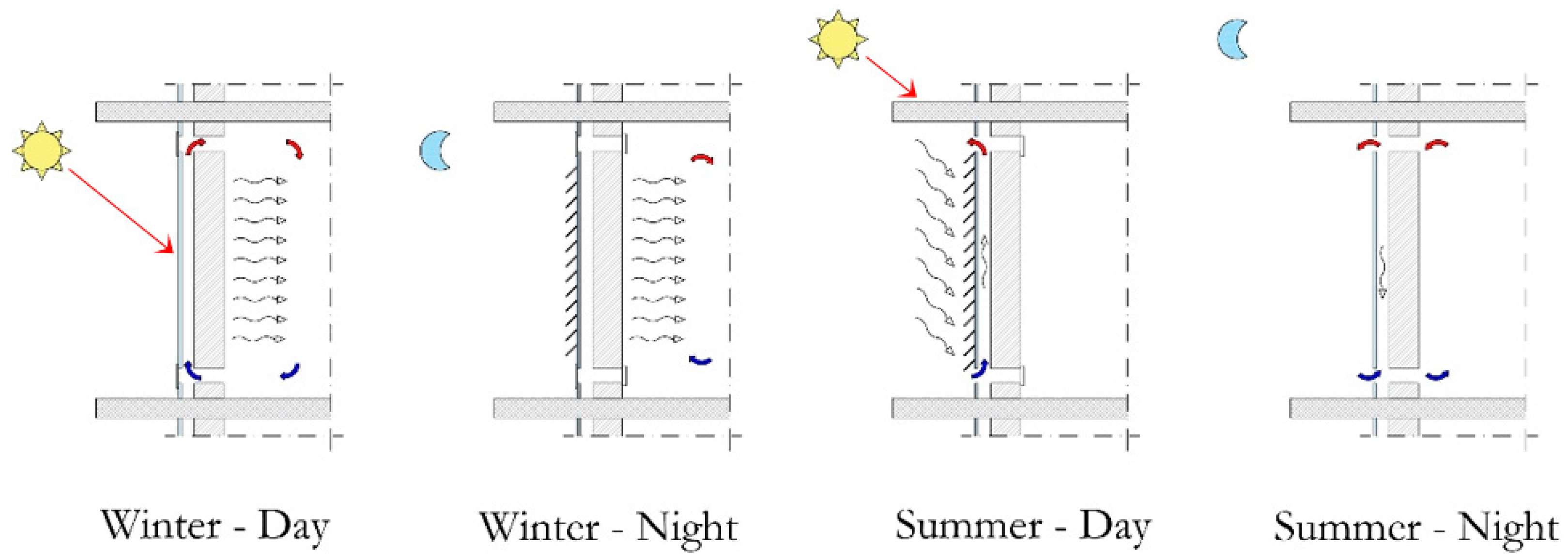
Figure 3.
3D view of the investigated reference building for the thermal performances of the Trombe wall.
Figure 3.
3D view of the investigated reference building for the thermal performances of the Trombe wall.

Figure 4.
Locality A: Solar saving fraction obtained for TWA3 (a) and TWD2 (b) with and without the installation of a PV generator during the heating months.
Figure 4.
Locality A: Solar saving fraction obtained for TWA3 (a) and TWD2 (b) with and without the installation of a PV generator during the heating months.

Figure 5.
Locality B: Solar saving fraction obtained for TWA3 (a) and TWD2 (b) with and without the installation of a PV generator during the heating months.
Figure 5.
Locality B: Solar saving fraction obtained for TWA3 (a) and TWD2 (b) with and without the installation of a PV generator during the heating months.

Figure 6.
Locality C: Solar saving fraction obtained for TWA3 (a) and TWD2 (b) with and without the installation of a PV generator during the heating months.
Figure 6.
Locality C: Solar saving fraction obtained for TWA3 (a) and TWD2 (b) with and without the installation of a PV generator during the heating months.


Table 1.
Main monthly average daily weather data of the simulated localities.
| Locality A—HDD 2248 (37.56° N, 14.28° E) | Locality B—HDD 2514 (42.21° N, 13.40° E) | Locality—HDD 2404 (45.46° N, 9.19° E) | ||||
|---|---|---|---|---|---|---|
| Month | Outdoor Temperature [°C] | South Incident Solar Radiation [kWh/m2 × day] | Outdoor Temperature [°C] | South Incident Solar Radiation [kWh/m2 × day] | Outdoor Temperature [°C] | South Incident Solar Radiation [kWh/m2 × day] |
| October | 17.9 | 3.64 | 12.6 | 2.86 | 14.1 | 2.31 |
| November | 12.4 | 3.42 | 7.8 | 2.22 | 7.5 | 1.49 |
| December | 9.3 | 2.92 | 2.7 | 2.11 | 3.5 | 1.67 |
| January | 8.5 | 3.98 | 3.0 | 2.53 | 4.0 | 2.19 |
| February | 6.7 | 3.85 | 4.3 | 3.23 | 7.1 | 2.56 |
| March | 9.1 | 3.60 | 8.1 | 3.33 | 10.6 | 3.04 |
| April | 12.7 | 2.83 | 11.0 | 2.82 | 13.4 | 3.00 |
Table 2.
Features of the Trombe walls implemented in TRNSYS simulations.
| Code | Thermal Capacity [kJ/m2 °C] | Massive Wall Thickness [m] | Density × Specific Heat × Conductivity [kJ2/s·m4·°C2] | External Cover Number | LCRS [kWh/m2·°C·day] |
|---|---|---|---|---|---|
| TWA2 | 459 | 0.23 | 3.470 | 2 | 0.0736 |
| TWA3 | 612 | 0.30 | 3.470 | 2 | 0.0736 |
| TWA4 | 920 | 0.46 | 3.470 | 2 | 0.0736 |
| TWB1 | 306 | 0.15 | 1.740 | 2 | 0.0736 |
| TWB2 | 459 | 0.23 | 1.740 | 2 | 0.0736 |
| TWB3 | 612 | 0.30 | 1.740 | 2 | 0.0736 |
| TWB4 | 920 | 0.46 | 1.740 | 2 | 0.0736 |
| TWD1 | 612 | 0.30 | 3.470 | 1 | 0.1247 |
| TWD2 | 612 | 0.30 | 3.470 | 3 | 0.0311 |
| TWE2 | 612 | 0.30 | 3.470 | 2 * | 0.0528 |
* low-ε inner glass.
Table 3.
Main electric features of the thin-film PV panels considered in simulations.
| Parameter | Value |
|---|---|
| Short-circuit current at STC | 2.20 A |
| Current at max power point in STC | 1.98 A |
| Open-circuit voltage in STC | 66.6 V |
| Voltage at max power point in STC | 53.5 V |
| Temperature coefficient of short-circuit current | 0.0015 A/K |
| Temperature coefficient of open-circuit voltage | −0.200 V/K |
| Efficiency at STR | 0.112 |
Table 4.
SSF determined by the Balcomb method (Balc.) and by transient simulations (TRN.) for two configurations of Trombe walls installed in the reference building located in the three considered localities.
Table 4.
SSF determined by the Balcomb method (Balc.) and by transient simulations (TRN.) for two configurations of Trombe walls installed in the reference building located in the three considered localities.
| Month | TWA3 | TWD2 | ||||||||||
|---|---|---|---|---|---|---|---|---|---|---|---|---|
| Location A | Location B | Location C | Location A | Location B | Location C | |||||||
| Balc. | TRN. | Balc. | TRN. | Balc. | TRN. | Balc. | TRN. | Balc. | TRN. | Balc. | TRN. | |
| October | 1.00 | 1.00 | 0.98 | 0.96 | 0.99 | 0.97 | 1.00 | 1.00 | 1.00 | 0.97 | 1.00 | 0.99 |
| November | 0.95 | 0.93 | 0.90 | 0.86 | 0.91 | 0.86 | 1.00 | 0.98 | 0.92 | 0.90 | 0.96 | 0.89 |
| December | 0.92 | 0.90 | 0.64 | 0.61 | 0.65 | 0.59 | 0.95 | 0.92 | 0.70 | 0.65 | 0.71 | 0.64 |
| January | 0.87 | 0.83 | 0.66 | 0.62 | 0.69 | 0.66 | 0.90 | 0.86 | 0.73 | 0.67 | 0.74 | 0.69 |
| February | 0.76 | 0.71 | 0.71 | 0.68 | 0.74 | 0.70 | 0.85 | 0.82 | 0.77 | 0.72 | 0.79 | 0.75 |
| March | 0.91 | 0.88 | 0.88 | 0.84 | 0.88 | 0.85 | 0.94 | 0.92 | 0.94 | 0.89 | 0.92 | 0.89 |
| April | 1.00 | 1.00 | 0.97 | 0.95 | 1.00 | 1.00 | 1.00 | 1.00 | 1.00 | 0.99 | 1.00 | 1.00 |
Table 5.
Values of the constants to adopt in the SLR approach with traditional and PV Trombe wall for different configurations of the passive system.
Table 5.
Values of the constants to adopt in the SLR approach with traditional and PV Trombe wall for different configurations of the passive system.
| Code | Traditional Trombe Wall | PVTW_M | ||||
|---|---|---|---|---|---|---|
| C | D | H | C | D | H | |
| TWA2 | 0.9680 | 0.6318 | 0.92 | 0.9687 | 0.4612 | 0.90 |
| TWA3 | 0.9964 | 0.7123 | 0.85 | 1.0121 | 0.5015 | 0.81 |
| TWA4 | 1.0190 | 0.7332 | 0.79 | 0.9898 | 0.4915 | 0.80 |
| TWB1 | 0.9364 | 0.4777 | 1.01 | 0.9714 | 0.3477 | 0.98 |
| TWB2 | 0.9821 | 0.6920 | 0.85 | 0.9569 | 0.4623 | 0.90 |
| TWB3 | 0.9980 | 0.6191 | 0.80 | 0.9679 | 0.4156 | 0.81 |
| TWB4 | 0.9981 | 0.5615 | 0.76 | 0.9901 | 0.3898 | 0.80 |
| TWD1 | 0.9842 | 0.4418 | 0.89 | 0.9723 | 0.3015 | 0.90 |
| TWD2 | 1.0150 | 0.8994 | 0.80 | 0.9841 | 0.5875 | 0.81 |
| TWE2 | 1.0476 | 1.0050 | 0.66 | 1.024 | 0.6568 | 0.68 |
Table 6.
Solar load ratio and solar saving fraction obtained for a TWA2 Trombe wall with and without PV panel installed on the massive surface.
Table 6.
Solar load ratio and solar saving fraction obtained for a TWA2 Trombe wall with and without PV panel installed on the massive surface.
| Traditional TW | Traditional TW | ||||||||
|---|---|---|---|---|---|---|---|---|---|
| Month | N | DD [°C × day/month] | S [kWh/m2 × month] | SLR | SSF | SLR | SSF | ||
| October | 31 | 0 | 57.1 | 0.60 | 60.93 | 0.00 | 0.0% | 0 | 0.0% |
| November | 30 | 132 | 47.0 | 0.64 | 59.51 | 4.10 | 92.7% | 4.11 | 85.4% |
| December | 31 | 233 | 42.5 | 0.66 | 53.58 | 1.78 | 68.5% | 1.79 | 57.6% |
| January | 31 | 257 | 44.7 | 0.65 | 72.34 | 2.31 | 77.5% | 2.32 | 66.8% |
| February | 28 | 283 | 53.3 | 0.62 | 60.14 | 1.59 | 64.5% | 1.60 | 53.7% |
| March | 31 | 239 | 64.6 | 0.54 | 54.40 | 1.75 | 67.9% | 1.76 | 57.0% |
| April | 30 | 123 | 72.3 | 0.43 | 32.67 | 2.15 | 75.0% | 2.16 | 64.2% |
Publisher’s Note: MDPI stays neutral with regard to jurisdictional claims in published maps and institutional affiliations. |
© 2022 by the authors. Licensee MDPI, Basel, Switzerland. This article is an open access article distributed under the terms and conditions of the Creative Commons Attribution (CC BY) license (https://creativecommons.org/licenses/by/4.0/).
Share and Cite
MDPI and ACS Style
Bruno, R.; Bevilacqua, P.; Cirone, D.; Perrella, S.; Rollo, A. A Calibration of the Solar Load Ratio Method to Determine the Heat Gain in PV-Trombe Walls. Energies 2022, 15, 328. https://doi.org/10.3390/en15010328
AMA Style
Bruno R, Bevilacqua P, Cirone D, Perrella S, Rollo A. A Calibration of the Solar Load Ratio Method to Determine the Heat Gain in PV-Trombe Walls. Energies. 2022; 15(1):328. https://doi.org/10.3390/en15010328
Chicago/Turabian StyleBruno, Roberto, Piero Bevilacqua, Daniela Cirone, Stefania Perrella, and Antonino Rollo. 2022. "A Calibration of the Solar Load Ratio Method to Determine the Heat Gain in PV-Trombe Walls" Energies 15, no. 1: 328. https://doi.org/10.3390/en15010328
Note that from the first issue of 2016, this journal uses article numbers instead of page numbers. See further details here.