
Automatic PRPD Image Recognition of Multiple Simultaneous Partial Discharge Sources in On-Line Hydro-Generator Stator Bars


Electrical Engineering Graduate Program, Federal University of Pará, Belém 66075-110, Brazil
*
Author to whom correspondence should be addressed.
Energies 2022, 15(1), 326; https://doi.org/10.3390/en15010326
Submission received: 3 November 2021
/
Revised: 25 November 2021
/
Accepted: 2 December 2021
/
Published: 4 January 2022
(This article belongs to the Special Issue New Trends in Condition Monitoring and Diagnostics of Power System Assets)
Abstract
:In this study, a methodology for automatic recognition of multiple simultaneous types of partial discharges (PDs) in hydro-generator stator windings was proposed. All the seven PD sources typical in rotating machines were considered, and up to three simultaneous sources could be identified. The functionality of identifying samples with no valid PDs was also incorporated using a new technique. The data set was composed of phase-resolved partial discharge (PRPD) patterns obtained from on-line measurements of hydro-generators. From an input PRPD, noise and interference were removed with an improved version of an image-based denoising algorithm previously proposed by the authors. Then, a novel image-based algorithm that separates partially superposed PD clouds was proposed, by decomposing the input pattern into two sub-PRPDs containing discharges of different natures. From the sub-PRPDs, one extracts features quantifying the PD distribution over amplitudes and the contour of PD clouds. Those features are fed as inputs to several artificial neural networks (ANNs), each of which solves a part of the classification problem and acts as a block of a larger system. Once trained, ANNs work collaboratively to identify an unknown sample. Good results were obtained, with overall accuracies ranging from 88% to 94.8% for all the considered PD sources.
1. Introduction
High-voltage electrical apparatuses are subjected to intense electrical, thermal, and mechanical stresses during operation [1], resulting in equipment aging. In aged rotating machines, including hydro-generators, partial discharges (PDs) occur in the stator insulation. PDs are local electrical discharges that do not completely bridge phase bars and the ground [2]. Partial discharges deteriorate the insulation progressively, and, in the absence of proper maintenance, eventually result in disruptive failures.
To avoid the great financial and operational losses of such incidents, power utility companies have resorted to partial discharge monitoring, deemed as the most effective technique for assessing the condition of stator insulation [3,4]. The idea is to track the actual health of machine insulation so that one can anticipate potential problems and plan for maintenance measures accordingly. This is in the context of condition-based monitoring, in which maintenance is performed only when necessary, based on the equipment’s actual condition [5].
Partial discharges have different characteristics depending on the type of insulation defect they occur in [2,3]. The task of determining the type of insulation defect based on the characteristics of PD patterns is called PD recognition. Knowledge of the PD source is very important in partial discharge monitoring systems [6] because the types of discharges impose different relative risks to insulation [7]. Given that partial discharges are a complex phenomenon, PD recognition is often done by experts [2,7]. Great research efforts have been made to automate the task of PD recognition, which would certainly help leverage condition-based maintenance of electrical equipment on a larger scale [8].
In rotating machines, partial discharges usually occur simultaneously at several insulation defects throughout the stator. The characteristics of each PD source will superimpose in the detected signal, resulting in a complex pattern. Another task in partial discharge monitoring is the rejection of patterns containing no valid PD source. Such a task reduces the rate of false alarms, which is important as it avoids the planning of unnecessary maintenance interventions. Patterns having only noise or very incipient discharges are too common to be ignored; they composed the majority of measurements in [4], for example. In [9], a methodology was proposed to recognize single-source PD patterns, including those containing only noise, in gas-insulated switchgear (GIS) using deep convolutional neural networks. Reference [10] proposed to identify noise by grouping discharges in different clusters in time-frequency maps.
The classification of patterns containing multiple simultaneous PD sources is an intricate problem [2,3]. It is usually solved with two main approaches.
In the first approach, one decomposes other types of input patterns (e.g., time-domain signals) using clustering techniques. Most discrimination methods are based on clustering features extracted from complex PD signals. Reference [6] proposed a new method to separate multiple sources. The smoothed density and density-peak-clustering techniques were combined to cluster discharges in the 2D space formed by the charge and energy of discharges. Time-domain signals are required to perform this separation. Work [11] describes a discrimination method of multiple simultaneous PD sources by clustering optimized features of the cumulative energy function of partial discharge signals. The method presented good performance when tested on signals from laboratory measurements and simulations. In [12], a multi-source PD separation algorithm was proposed based on linear prediction analysis and the isolation forest technique. Linear prediction is used to create a feature space by approximating each data point of PD signals as a linear combination of previous points. The isolation forest quantifies the degree of clustering by calculating the height score metric. Multiple PD sources are separated by grouping PD signals with fuzzy C-means clustering technique, in the 3D space formed by two features from the linear prediction plus the height score. The method was tested on measurements from laboratory models, and good results were achieved.
In the second approach, one applies artificial-intelligence algorithms to phase-resolved partial discharge (PRPD) matrices or image patterns but without using clustering. The work of Lalitha and Satish [13] was the first to propose multi-source PD recognition based on PRPD images. Single-source PD measurements were taken in laboratory conditions and were superposed onto one another to create an artificial data set of multiple-source PRPDs. Those PRPDs were decomposed with 2D wavelet transform, and features were extracted and fed to radial basis neural networks for classification. Recognition rates of about 86% were obtained. Reference [14] presents a methodology for the PD recognition of two simultaneous sources in medium-voltage motors. Fractal features were extracted from the typical PRPDs of standards [15], and the resulting fractal map was used as a reference. When presented to an unknown PRPD, the same fractal features were extracted, and they were compared to the reference map using the Center Score algorithm, which estimates the probabilities of belonging to each PD source. In [3], a method for recognition of up to three simultaneous types of PD was proposed. Fractal features were extracted from PRPD patterns using image-processing techniques and then inserted as inputs to a non-linear multi-class support vector machine for classification. The database was composed of measurements taken from artificial laboratory models. Work [16] proposes the use of an improved convolutional neural network (CNN) to classify single and multiple PD sources using only single-source patterns in the training set. The proposed architecture consists of a CNN followed by multiple fully connected networks, each specialized in identifying a different PD source. The input patterns were PRPDs obtained from measurements in artificial models in laboratory. Six types of PDs were considered, and the proposed CNN was able to classify up to three simultaneous PD sources. The two works mentioned represent the main options available for PD recognition: machine learning [3] or deep learning [16]. Machine learning is the traditional method of first extracting from the raw data manually predetermined features, which are then used as inputs to classifiers. In deep learning, the raw data are directly passed to classifiers, which automatically learn a subset of features and use it to identify the sample. Many works in the literature report that deep-learning-based classifiers outperform their machine-learning counterparts only when the database is relatively large [9,17]. This is expected by theory because, since deep classifiers usually have more hyperparameters, they are more prone to overfitting, and, to compensate for that, more training samples are necessary for adequate generalization of the problem. Due to the complexity of partial discharge measurements and limited access to real-world machines, it is hard to build large PD databases [17].
There are some shortcomings in the mentioned works, as well as in the overall literature on PD monitoring. First, most studies trained and tested their recognition methodologies with artificial models in laboratory conditions. Signals collected in these conditions were less infected by noise and interference; hence, the statistics calculated overestimated the accuracies that would be obtained in real-world online conditions [9]. The work [16], for example, reported recognition rates greater than 96%, but this metric was calculated on patterns obtained in laboratory conditions with very little noise. Such high recognition rates might be unrealistic for online measurements in hydro-generators, which is a much harder problem. Another disadvantage is that usually up to six PD sources are differentiated, which does not cover all possible types. Additionally, most recent advancements in PD denoising and separation of multiple sources rely on the time-domain PD signals, which may not be available in storage-constrained applications due to the high sampling rate required to record these signals. Finally, the majority of studies do not seem to have the functionality of identification of patterns with no valid PD source.
This study mitigates many of those limitations. We propose a methodology that is capable of classifying multiple simultaneous PD sources, including the functionality of recognizing samples not having valid PD activity. The data set was formed of PRPDs obtained from measurements in online hydro-generators containing multiple simultaneous PD patterns. Noise and interference were removed with a modified version, tailored for the multiple-source case, of our previous work’s denoising algorithm [18]. For this purpose, partial discharges were clustered in different groups in each PRPD, which is a contribution. Moreover, a new algorithm separates PD clouds, even if they are partially superposed, and its output is the input sample decomposed into two sub-PRPDs containing discharges of different natures. Features are extracted from the sub-PRPDs, including a novel attribute that quantifies the shape of PD clouds. The classification task was decomposed into smaller problems, each solved with an artificial neural network (ANN) trained with one of those features. All the algorithms in the methodology treat PRPDs as images. To the best of our knowledge, this is the first study to develop a method combining all these functionalities. The proposed methodology achieved good performance on the tested samples, with accuracies ranging from 88% to 94.8%.
The motivation of this work was to propose an algorithm combining, for the first time, many functionalities that are necessary for the classification of multiple simultaneous PD types in hydro-generators operating in real-world conditions, which is of great interest to power utilities. For that, the contributions of this study are the following:
- a novel recognition method of multiple simultaneous PD sources;
- the development of a new input feature that quantifies the shape of PD clouds;
- the proposal of a new algorithm to detect invalid samples, which contain no readily identifiable PD source;
- a new method of separation of multiple PD sources partially superposed in the PRPD image.
2. Data Set Obtained from Online PD Measurements in Hydro-Generators
The data set used in this work was built the same way as in our previous study [18] but with some important differences. It is composed of online PD measurements from hydro-generators of the Tucuruí and Coaracy Nunes power plants (Northern Brazil).
Measurements were performed as described in [18]. Capacitive couplers were used as PD sensors. Signals picked up by the sensors were digitized with the NI-USB 5133 oscilloscope and then processed by the Instrumentation for Monitoring and Analysis of Partial Discharges (IMA-DP) [19] acquisition setup. In each measurement, the signal was acquired for 700 AC cycles; all PDs detected during this interval appeared as high-frequency pulses in the signal. IMA-DP scans for all the peaks in the captured signal and registers the number of peaks as a function of their amplitude and the phase angle of the AC cycle at which they occurred in patterns called PRPDs. IMA-DP performs this mapping by discretizing each of the amplitude and phase ranges in 256 equal bins, resulting in 256 × 256 PRPDs. Mathematically, PRPD is a matrix whose element at index is the quantity of PDs detected during acquisition whose peaks lie within the i-th amplitude and j-th phase angle bins. PRPDs are what constitute the database.
The generators of the Tucuruí power plant have different power ratings and construction designs compared to those at Coaracy Nunes. Additionally, the data set was built of measurements taken over many years, at different seasons of the year and at several times of the day. Thus, measurements represent multiple conditions of operation of different types of machines, captured at different stages of their aging process. The result is that the database is statistically representative of the phenomenon of partial discharges in rotating machines. Automatic PD-recognition algorithms that perform well on this data very likely have generalized the task of classification (good accuracy on new samples).
The PRPDs’ true PD sources were manually labeled by a human expert among the types of PD commonly found in rotating machines [15,20]: internal void (InV), internal delamination (InD), delamination between conductors and insulation (DCI), slot, corona, surface tracking (Trk), and gap discharges (Gap). Figure 1 shows clear PRPDs (little contamination with interference and noise) associated with each one of these sources. The manual labeling was performed considering the expert’s knowledge of the generators and the PRPD characteristics correlated with the underlying PD source, which are the symmetry of PDs in positive and negative polarities and the shape of PD clouds [15,20].
Figure 2 shows the PD source distribution in the data set. Unlike the data sets of [18], there were patterns with multiple simultaneous PD sources and also a great number of unidentified (Und) samples. Und patterns do not present valid PD sources; there is only noise, or the PD clouds are so malformed (low height, density, etc) that they were not considered valid by the specialist during labeling. Another remarkable difference from [18] is the absence of merged PD sources, i.e., every one of the considered PD types can be distinctively identified by the recognition system developed here, whereas, in [18], the samples of some PD sources were treated as belonging to the same class (merged). This is because of a new input feature proposed in this study, which is able to differentiate between slot and corona and between internal void and internal delamination based on the shape of PD clouds.
Because PRPDs are from online measurements, they are contaminated with many types of interference and noise [21]. All of the disturbances in the data sets of [18]—intense noise, crosstalk, and an ambiguous shape of PD clouds—were also present here. These disturbances, combined with the presence of multiple simultaneous sources, are exemplified by the PRPDs of the data set shown in Figure 3 and greatly increased the difficulty of automated PD recognition; such obstacles cannot be avoided and are very common in online measurements; therefore, any classification methodology to be of practical use must be robust enough to deal with them. The recognition methodology proposed in this study is able to tackle all these obstacles.
3. Proposed Recognition Methodology of Multiple PD Sources
3.1. Overview
Before presenting the methodology, it is important to review some terminology defined in our previous study [18]. The noise gap is the horizontal band around amplitude zero without PDs. ANGPD discharges (an acronym for “Adjacent to Noise Gap PDs”) are close to the noise gap, and the other discharges are called N-ANGPD (Non-Adjacent to Noise Gap PDs). ANGPD clouds are candidates to belong to PD sources InV, InD, DCI, slot, and corona, whereas N-ANGPD discharges are potential surface tracking and gap sources. PDs termed higher or lower have higher or lower absolute amplitudes than others. Those terms are illustrated in Figure 3.
The common PD sources in rotating machines produce PRPDs typically characterized according to Table 1 [15,20]. Following the categorization of Table 1, it is possible to classify PD sources using a two-step process. First, a preliminary separation can be performed based on the symmetry between positive and negative PDs, and then the PD clouds’ shape is considered to resolve between sources with the same symmetry information. The proposed PD recognition methodology was structured with that same reasoning.
In this study, a PD-recognition methodology that is able to identify a single or multiple typical sources in rotating machines is proposed. It is capable of identifying up to three simultaneous PD types: the dominant ANGPD source plus surface tracking and/or gap discharges. The dominant ANGPD source is the one associated with the pair of positive and negative ANGPD clouds with the highest number and density of PDs. Gap-discharge clouds are detected even if they are partially superposed onto the ANGPD clouds. The absence of ANGPD and/or N-ANGPD sources can also be detected. The technique is an extension of those previously proposed by the authors in [18,22]; it operates entirely on PRPD patterns, which are treated as images.
During this research, we did not find a feature that would single-handedly be capable to accurately differentiate between all the typical PD sources mentioned in IEC 60034-27-2 [15]. Therefore, the recognition task was divided into smaller problems. This approach usually results in shorter training times and better generalization due to the simpler individual classifiers [23].
The proposed methodology is based primarily on fully-connected feedforward artificial neural networks. It consists of training, validation, and testing stages. In the first two phases, different ANNs are trained so that each solves a smaller problem of the classification task in an isolated manner. In the testing stage, the previously trained ANNs are combined hierarchically to perform PD recognition on unknown samples.
The training and validation stages are illustrated by the block diagram of Figure 4. First, the input pattern is subjected to a PRPD image-denoising algorithm for suppressing spurious discharges that are not related to the underlying PD source(s). The algorithm is based on our proposal of [18] but with some modifications to address the multiple-source case (Section 3.2). Next, a novel image-processing technique is applied to separate horizontal N-ANGPD clouds partially superposed onto the ANGPD discharges (Section 3.3). The image denoising yields groups (clusters) of denoised N-ANGPD and ANGPD discharges. From these groups, two sub-PRPDs are generated: one containing only N-ANGPD PDs and the other with only ANGPD clusters.
From the patterns known to have surface tracking and/or gap activity (as labeled by the specialist), the clouds of their N-ANGPD sub-PRPDs were used to optimize the thresholds of a manually predetermined set of rules (Section 3.5). In the testing stage, those rules are used to identify the presence of such PD sources by analyzing the dimensions and positions of a PRPD’s N-ANGPD clouds.
The dominant ANGPD PD source is identified by the cooperation of four types of neural networks: ANNs-0, ANNs-1, ANNs-2, and ANNs-3. Some of their hyperparameters are listed in Table 2; the topology (number of hidden layers and hidden neurons) is determined heuristically in Section 4.2. As detailed in Section 3.8 and Section 3.9, the networks were trained and tested with several combinations of mutually exclusive subsets of training, validation, and test data. The numbers of PRPDs forming those subsets are also listed in Table 2 for each network type.
From the ANGPD sub-PRPD, neural network ANN-0 detects whether the pattern’s ANGPD clouds are noisy by analyzing simple cloud characteristics such as height and density (Section 3.7). Next, the ANGPD sub-PRPDs with a valid ANGPD PD source (as labeled by the specialist) are partitioned into different subsets (Section 3.8) to train other three types of neural networks, each fed with one of the input features: amplitude histograms [18] and the novel contour attribute, described in Section 3.6. The first neural network (ANN-1) uses histograms to perform preliminary recognition, by merging InV with InD patterns (class InV/InD) and slot with corona (Slot/Corona) into two different groups of samples. Those mergers are necessary because the histogram does not accurately capture the differences in cloud shape that differentiate those classes [15,18]. The other neural networks (ANN-2 and ANN-3) solve these ambiguities with contour features, which are more sensitive to the cloud shape.
The testing stage is illustrated in Figure 5. An input pattern is subjected to the algorithm of noise removal and multiple source separation (Section 3.2 and Section 3.3). In the N-ANGPD sub-PRPD, one looks for surface tracking and gap PDs by comparing the dimensions and positioning of its clouds against predetermined thresholds. From the ANGPD sub-PRPDs, several metrics were extracted and used by the ANN-0 network to estimate whether ANGPD clouds are noisy or valid. If both clouds are deemed as noisy, it is considered that there is no ANGPD PD source in the pattern. If at least one cloud is judged valid, the pattern is classified by a cascade of trained networks ANN-1, ANN-2, and ANN-3. ANN-1 identifies the sample based on its amplitude histogram. If ANN-1’s output is DCI, this already is the system classification for the ANGPD PD source, since this class is characterized solely by the symmetry between positive and negative PDs (Table 1) [15,20]. If ANN-1’s output is InV/InD or slot/corona, contour features are calculated and passed to the corresponding auxiliary neural network (ANN-2 or ANN-3) to solve the ambiguity.
Keeping the practice of [18] of describing the algorithms independently from the PRPD dimensions, in this study, the parameter values of the denoising and multiple-source separation algorithms are described as functions of the number of pixels A forming the width/height of a PRPD pattern. In the case of this study, .
3.2. Modifications to the Denoising Method of Our Previous Work
The denoising algorithm used in this study was based on the description of [18] but with some adaptations to better suit PRPDs with multiple simultaneous types of discharges. The denoising algorithm is shown in Figure 6, highlighting which steps were modified or added relative to the description of [18].
The noisy PRPD was subjected to two independent filtering paths, one tailored for low-density N-ANGPD clouds (pixel submatrix filtering) and the other for ANGPD discharges (four steps in this study). The steps of ANGPD phase delimiting and removal of non-dominant ANGPD s rely on rough contours (), which are functions of phase that estimate the amplitude of the boundary between ANGPD and N-ANGPD discharges at each phase angle. The ANGPD phase delimiting stage operates on smooth contours (), which are equal to the filtering of rough contours with exponential moving averages (), followed by a linear transformation to change its values from row coordinates to absolute amplitudes [18].
Rough contours are functions of a free parameter g. Smaller g produces rough contours passing at lower amplitudes. The first modification is that, in this study, rough contours were calculated with in ANGPD phase delimiting and with in the removal of non-dominant ANGPD s, whereas, in [18], was used for both of those stages. The values of g in both steps are smaller so that rough contours do not encompass low-amplitude N-ANGPD clouds, a common situation in this database. Different values of g were used also because of the different goals of the steps: in the ANGPD phase delimiting step, the rough contour needs to follow the high-density discharges of ANGPD clouds to obtain accurate phase bounds, and, in the next step, the noise of low- and medium-amplitudes must be removed to better isolate the ANGPD clouds from spurious PDs.
The second difference is that a new step of separation of multiple N-ANGPD discharges (Section 3.3) was added following the removal of non-dominant ANGPD s. The two filtering paths produced two partially denoised patterns and (Figure 6). The third and last difference is that, in this study, those patterns were combined to form two sub-PRPDs: one containing only N-ANGPDs, and the other formed only by ANGPD discharges (Section 3.4). In [18], a single PRPD containing only one dominant PD source was generated.
3.3. Separation of Superposed N-ANGPDs
In this stage, illustrated by the namesake block in the blue of Figure 6 and detailed in Figure 7, the separation between partially superposed horizontal N-ANGPD (potential gap discharges) and ANGPD clouds in the PRPD image was performed, a common situation in the database. The separation was based on the fact that N-ANGPD clouds usually have PD counts higher than the ANGPD clouds at the intersection region.
After the removal of non-dominant ANGPDs (Figure 6), PDs were grouped by means of nearest-neighbor clustering [24] using a 0.05A × 0.05A pixel submatrix. Figure 8b shows the results of clustering applied to the pattern of Figure 8a, which in turn is the PRPD of Figure 3d after the removal of non-dominant ANGPDs. Each cluster is indicated with its PDs in a different color.
The following algorithm was applied to each ANGPD cluster separately. From the PRPD, a matrix containing only the PDs of the cluster being analyzed was formed. This matrix was divided into a grid of cells. One calculates matrix M, whose elements are equal to the sum of PD counts within each cell of the grid. Matrix D was then obtained by normalizing M by its maximum non-zero element excluding outliers. Figure 8c, for example, shows the matrix D relative to the positive ANGPD cluster of Figure 8b.
In order to remove as much superposition as possible, it is necessary to estimate the actual dimensions of the superposed N-ANGPD clouds (if any). For that, we exploited the fact that PD clouds are usually formed by higher-count discharges in the central region, surrounded by smaller-count discharges. If only the high-count PDs are considered, one obtains smaller versions of the superposed N-ANGPD clouds whose boundaries (formed by the furthermost discharges from the cloud’s center) are farther from one another, facilitating their identification as separate groups. From the identified higher-count portion of the superposed N-ANGPD clouds, it is easier to estimate their actual dimensions. The separation algorithm developed in this study follows such reasoning.
It is convenient to introduce the matrix , given by
where L is a real-valued number from 0 to 1 that sets the threshold of the minimum normalized PD count considered. For a given value of L, the matrix is formed, and its non-zero pixels of are grouped with nearest-neighbor clustering [24] using a 0.0195A × 0.0195A submatrix. One determines the bounding box (BB) of each cluster, which is the smallest imaginary rectangle (height is H and width is W pixels) containing all the cluster’s discharges. In Figure 8d, for example, the BB of the cluster in red is shown. ’s N-ANGPD clusters are scanned, and those meeting and are considered horizontal. This is repeated iteratively varying L in the sequence {0.70, 0.50, 0.40, 0.30, 0.20, 0.15, 0.10, 0.08, 0.05, 0.02, 0.00}, in a process called the loop of thresholds. On the course of this loop, gradually rebuilds matrix D, from the highest-count pixels to those of smallest-count, as seen in Figure 8d–f. In the initial iterations (high L), there are only the innermost high-count PDs of each cloud, and thus those groups tend to be separated (Figure 8d). As L decreases (Figure 8e–f), the groups’ boundaries progressively approach each other, eventually forming a single cluster again. For each horizontal N-ANGPD cloud detected during the loop, let be the corresponding cluster in matrix for the smallest L at which the N-ANGPD and ANGPD clusters are still separated. Based on the clusters, one separates N-ANGPD clouds from the ANGPD cloud with the procedure explained below, illustrated in Figure 9, Figure 10 and Figure 11. If no horizontal cloud is found at any of the L thresholds, it is assumed that there are no superpositions, and no separation is performed for the current ANGPD cloud. The loop of thresholds is then repeated for the other ANGPD clusters of the PRPD, one at a time.
The horizontal clusters detected in the loop of thresholds underestimate the dimensions of superposed N-ANGPD clouds. For a more accurate estimation, the bounding box of each cluster was “expanded” using the following procedure, illustrated in Figure 9 for the pattern of Figure 8. Such expansion occurs iteratively in matrix D, in the vertical and horizontal directions, while the PDs within the expanded BB are distributed similarly to the PDs bounded by ’s original BB. For each column of ’s original BB, one calculates the proportion of the non-zero elements () relative to the total number of pixels in the column and the average of the row coordinates of the non-zero elements weighted by its values in matrix D (), as shown in Figure 9b. The averages of those metrics over all the columns of the original BB are and . In the horizontal direction, the BB’s left bound is shifted to the left, one column at a time, while the relative differences between the and values in the new column and and are less than 75% and 40%, respectively. The same is performed to the BB’s right bound. An analogous procedure was then applied in the vertical direction. The pixels within the expanded BB were estimated to form the actual N-ANGPD cluster (pixels in green in Figure 9a).
The proposed separation algorithm deals with two types of superposition. Case 1, common in the database and illustrated in Figure 10a (original PRPD shown in Figure 3e), consists of a wide horizontal group above the ANGPD cloud, both connected by noisy pixels of low/intermediate density. In case 2 (Figure 8a), there is an actual superposition between the horizontal N-ANGPD and ANGPD clouds.
Each case is treated differently. Thus, it is necessary to identify to which category the superposition between ANGPD and N-ANGPD clouds belongs to. In the region bounded by the superposed cluster’s BB, 0.08A equally spaced columns of elements of matrix D (vertical profiles) were sampled along the phase axis, as shown in Figure 10b. The point-wise average of those 0.08A curves resulted in the average vertical profile, illustrated in Figure 10c. The average vertical profile can be seen as a function describing the average distribution of PD counts across amplitudes. For case 1, this function should have, in the direction from the ANGPD cloud to N-ANGPD discharges, a sequence of a local maximum, minimum, and maximum, respectively, associated to the ANGPD clouds, noise, and horizontal PDs (Figure 10c). In this study, the local minima and maxima were found by iteratively sliding a 0.02A-element-wide window along the average vertical profile. The central point is a local maximum if it is the largest element inside the window, or it is a local minimum if it is the smallest. Moreover, since horizontal PDs span a phase interval comparable to the ANGPD cloud’s width in case 1, little variation between the individual vertical profiles was expected. This variation was quantified inversely by the similarity , calculated as the average of the cross-correlations between all the pairwise combinations of vertical profiles. Based on this information, the superposition was considered to belong to case 1 if all the following criteria were met: (i) N-ANGPD cloud is horizontal; (ii) ; and (iii) the average vertical profile presents exactly three local extrema, one minimum between two maxima, and that the minimum has a value less than 1% of the first maximum’s. Otherwise, superposition was considered to be of case 2.
The following explanations were described based on the x and y axes (Figure 10 and Figure 11). The x-axis is horizontal, oriented left-to-right in the PRPD. The y-axis is vertical, oriented from the bottom to the top of the superposed cluster.
In the case-1 superposition, let and be the y coordinates of the upper and lower bounds of the intermediate noisy region, respectively (Figure 10b). Due to the small number of discharges in this zone, the average vertical profile function assumes lower images in this region (rows ) than in the other two regions, which are associated with the ANGPD and horizontal clouds (Figure 10c). It is considered that matches the lower bound of the horizontal cloud’s expanded BB. Moving in the direction of decreasing y, the first row at which was estimated as the coordinate . The coordinates and are illustrated in Figure 10b,c. Additionally, let and be the x coordinates of the left and right bounds of the ANGPD cloud, and let be the y coordinate of this cluster’s lower bound (Figure 10b).
Next, one calculates the vectors and , containing the x coordinate of the cluster’s leftmost and rightmost non-zero pixel in each row, respectively, (red and green curves in Figure 10b). The left and right contours of the ANGPD cloud were estimated by fitting parabolas to certain points of the curves and using the least squares method. Such parabolas must be convergent—that is, they must intersect at a point whose x coordinate is within —and the intersection point determines the ANGPD cloud’s upper bound. It is estimated that the ANGPD cloud’s peak lies next to the central point of the noisy region, where and . Parabolas were fitted to the points of and corresponding to the set of rows , where was initially equal to . If parabolas are not convergent, new fitting attempts are performed by iteratively decreasing , one row at a time, until the convergence of parabolas is achieved. If there is no such that the parabolas intersect at a point above the expanded horizontal cloud’s lower bound, the fitting was not adequate, because it violates the hypothesis of no superposition between the clouds. In this case, new parabolas are fitted to the points of and corresponding to the set of rows , and also to the point . The addition of this point tends to induce the expected convergence of parabolas. In the example of Figure 10d, the parabolas were obtained in the first fitting attempt to the points of and of the rows . Separation was performed by assigning to the ANGPD cloud the PDs below the fitted parabolas, and the horizontal cloud was composed of the PDs within its expanded bounding box (Figure 10e).
For case-2 superpositions, the and curves of the cluster were also calculated in matrix D (Figure 11a). In the absence of disturbances, and tend to vary monotonically along the x-axis. When there are superposed horizontal clouds, however, those curves experience sharp variations along x in the opposite direction to what is expected (“divergences”), as shown in Figure 11b. Disregarding the points of and associated with the divergences caused by superposed horizontal clouds (diverging points), it is possible to estimate the ANGPD cloud’s left and right contours without superpositions.
Figure 11 illustrates the separation of case-2 superpositions for the positive ANGPD cluster of the pattern of Figure 8a. One obtains the local maxima (tops) and minima (bottoms) of and curves (Figure 11b). In the and curves, one finds the local maxima (tops) and minima (bottoms) within the 2-point distance. For more robustness against noise, one considers only the pairs of consecutive local minimum and local maximum whose x values differ by at least nine pixels. Each sequence of three local extrema (top-bottom-top for , or bottom-top-bottom for ) was assumed to be related to the superposition with a horizontal cloud. The superposed horizontal clouds may have counts different or similar to the ANGPD cloud’s in the region of intersection. In Figure 11a, for example, the superposed horizontal PDs to the right (purple arrow) and to the left (yellow arrow) were of the first and the second type, respectively. The diverging points of and were determined for each triplet of local extrema.
For each horizontal cloud of distinctive count (expanded cluster ), detected during the loop of thresholds, one verifies to which sides it causes divergence in the ANGPD cloud. Let and be the y coordinates of the upper and lower bounds of ’s BB (Figure 11a). In and , it was verified if there is a triplet whose first and third local extrema have y coordinates less than and greater than , respectively. In Figure 11c, for example, this applies to the triplet in . If such a triplet exists in , and if the element of immediately below the horizontal cloud has x value () between the left and right bounds of , the points of corresponding to the rows are divergent (Figure 11c). Analogous logic applies to .
The other triplets of local extrema may be related to superpositions of horizontal clouds not detected during the loop of thresholds. The following procedure was performed for each of those triplets. Let F be the curve or to which the triplet in question belongs, and let be the coordinates of the first local extremum in F (Figure 11c). Starting from this extremum and moving in the direction of increasing y, one looks for the first point of F such that if , or if . The point is shown in Figure 11c. The determination of this point follows the assumption that, in the direction of increasing y, once one gets past the divergence, ’s x values are again greater than (or less than if ) , an indication that the ANGPD cloud resumed its natural trend of narrowing in the phase axis. In order to reduce the influence of noise, the points of F in the rows were considered divergent only if all the following criteria were met: (i) there are at least two points of F between the first and third local extrema of the triplet; and (ii) the magnitude of the difference between and the median of the x values of F in the interval is greater than or equal to 12. In Figure 11c, the triplet of local extrema of meets these conditions.
Using least squares, parabolas were fitted to the and curves disregarding the divergent points, as shown in Figure 11c. For each group of divergent points of the curve F ( or ), the PDs of y coordinates equal to the divergent points and not contained by the parabola fitted to F (to the left of the parabola if , or to the right if ) were removed from the ANGPD cluster and assigned to a new N-ANGPD cluster. The hatched areas in Figure 11c indicate the regions in which PDs were separated from the ANGPD cloud. Figure 11d shows the separation of superposed horizontal and ANGPD clouds.
At this moment, the N-ANGPD clouds superposed onto a single ANGPD cluster were separated. The entire separation process (the calculation of matrix D, the loop of thresholds, and so on) was repeated for the PRPD’s other ANGPD clusters, one at a time. Finally, the pixel coordinates of all the separated clusters were mapped back to the PRPD’s original dimensions . The values of thresholds described in this subsection were defined empirically, in order to separate most of the superposed patterns in the database.
Superposed tracking PDs could be separated in a way analogous to the case-2 superposition. Instead of and , the procedure would be based on curves containing the y coordinates of the cluster’s uppermost and lowermost non-zero pixel at each column. However, due to the low occurrence of this type of superposition in the database, the separation of tracking clouds was not implemented in this study.
3.4. PRPD Decomposition
The separation of multiple sources was the last of a sequence of four steps focused on removing as much noise as possible from ANGPD clouds, producing a partially denoised pattern (Figure 6). There was a second filtering path tailored for preserving low-density N-ANGPD discharges (pattern ). In the current step of PRPD decomposition, illustrated by the namesake block in blue of Figure 6, and were combined to form two sub-PRPDs.
Nearest-neighbor clustering [24] was applied separately to and , using a submatrix of × pixels, the same dimensions adopted in [18]. Figure 12a,b illustrates the results of clustering on the partially denoised versions and of the PRPD of Figure 3d. Discharges of each cluster are shown in a different color.
PDs of and were combined to produce two sub-PRPDs: one containing only ANGPD and the other only N-ANGPD discharges (Figure 12c,d). The ANGPD sub-PRPD was composed of ’s ANGPD clusters. The N-ANGPD sub-PRPD was formed of the union of PDs belonging to ’s and ’s N-ANGPD clusters.
3.5. Classification of N-ANGPD PD Sources
Given the characteristic format of gap and surface tracking sources [15], in this study, those types of PD were identified by directly comparing the dimensions and relative positions of the sub-PRPD’s N-ANGPD clouds against predetermined thresholds, without using artificial intelligence (AI).
The BB of each cluster of N-ANGPD sub-PRPD was determined; its width and height were W and H pixels, respectively (Figure 12c). One considers the presence of tracking activity in a pattern if there is any cluster whose BB meets , , and the proportion of non-zero pixels within the BB (a measure of density) is greater than 12.6%. The gap discharge source is detected if there is a pair of horizontal clouds, one in each polarity, of approximately the same magnitude amplitude (maximum 16% relative difference between the clouds’ centers amplitudes) and approximately 180 apart from each other in the phase axis (phase distance between clouds’ centers within ). A cluster is deemed horizontal if its BB meets and . The informed values of thresholds were optimized to maximize the system’s classification rates of surface tracking and gap PD sources, as discussed in Section 4.
3.6. Extraction of Contour Features
As already mentioned, the PD-recognition task was divided into smaller problems using two input features: amplitude histograms [18] and the novel contour attribute, which quantify the PD symmetry and cloud contours, respectively. Those characteristics, besides being mentioned in the literature to describe typical PRPDs of different sources [15,20], are also considered robust to variations in measurement conditions [25].
The contour attribute is a novel contribution of this work. This feature quantifies the shape of PD clouds, which is the main difference between InV and InD classes and between slot and corona [15,20]. It is considered the contour of only the positive ANGPD cloud. The negative cloud is ignored because it is redundant for InV, InD, slot, and corona sources.
Figure 14 shows ideal triangular and rounded ANGPD clouds, alongside the first derivative of the mathematical function describing the cloud’s contour. The distinctive variations of the first derivatives demonstrate that these curves may be used to efficiently quantify the shape of PD clouds. PRPDs obtained from online measurements have clouds with irregular and noisy contours, whose derivatives differ to a certain degree from those shown in Figure 14. In this study, neural networks learn from real data the differences between the first derivatives of both types of curves.
In order to obtain the contour feature, one first calculates the preliminary contour () of the positive ANGPD cloud. For each phase angle between this cloud’s phase bounds, is equal to the average of the row coordinates of the six highest non-zero PDs in that column. was subjected to a low-pass Butterworth filter [26] of order 5 and normalized cutoff frequency 0.1. The first derivative of the filtered was calculated, which was then smoothed by a second Butterworth filter of order 2 and normalized cutoff frequency 0.04. After sampling 32 equally spaced points from the smoothed derivative and applying min-max scaling to the range, one obtains the feature vector. The chosen length of the feature vector provides a balanced compromise between contour resolution and neural network complexity.
Figure 15 shows the contour feature calculated for one InV and one InD sample of the database. Despite the irregular ANGPD clouds, representative contours (in purple) were extracted. It is important to note that features also resemble the derivatives of the corresponding ideal contours (Figure 14). The informed values of parameters used to calculate , its derivative, and smoothing filters were determined by parametric tuning.
3.7. Identification of Noisy ANGPD Clouds
This step aimed to identify patterns whose two dominant ANGPD clouds were noisy, a common situation in the database (Figure 2). Such a stage adds to the system the important capability of identifying patterns not having a valid PD source, increasing its applicability in practical situations due to the reduction in false positives. Without this functionality, patterns with noisy ANGPD clouds would always be assigned to one of the ANGPD PD sources by neural networks.
Figure 16 shows typical cases of patterns with no valid ANGPD clouds. The most common situations are clouds of low density and/or low height. The other cases are clouds whose height and/or density are very similar to those of PDs in other phases (it is expected that such characteristics of valid ANGPD clouds are higher than in other phases, which are presumably occupied by noise only).
These situations are identified by capturing the following attributes of a pattern’s ANGPD clouds: height (H), density (), the height–width ratio (), contour variance (), signal–noise ratios of height (), and density ().
The characteristics were extracted from rough contour (Section 3.2) [18], which was calculated with specific values of g and on different versions of the pattern. was calculated with for H, , and , and with for the other attributes. Using the corresponding g, the rough contour was calculated on PRPD after grid filtering for and . For the other attributes, was calculated on the ANGPD sub-PRPD.
Before explaining how attributes are calculated, it is convenient to present some definitions. Let and be the columns of ANGPD cloud’s left and right phase bounds (e.g., vertical dashed lines in Figure 15), respectively. The height of PDs over a given phase interval is the 80th percentile of the values of smooth contour (Section 3.2) within this interval. The PD density is the proportion of non-zero PDs within a given phase interval and below the EMA-filtered rough contour (–Section 3.2).
H and are the height and density of PDs within the phase interval , respectively. is the cloud’s height divided by its width, which is equal to the smallest phase distance between and . is the subtraction between the cloud height and the height of PDs in the other phases (). is the cloud density divided by the density of PDs in the other phases. is the variance of values within phases and min-max normalized to the range .
From the ANGPD sub-PRPD, a pair of values was calculated for each attribute: one from the positive cloud and one from the negative cloud. The feature vector, which is presented to ANNs-0, is formed by the maximum of each of those pairs.
3.8. Data Partitioning
ANGPD sub-PRPDs of patterns with labeled ANGPD source (Figure 4) were randomly divided into mutually exclusive subsets with five-fold cross-validation (CV) [27]. CV generates several data partitions, each of which is a selection of three folds for training: one for validation and the others for testing. All the 20 possible partitions were considered.
CV partitions used by ANNs-1 were obtained by merging the subsets of InV with InD of each fold into a single class. The same was done for slot and corona patterns. Partitions for ANNs-2 consisted only of the InV and InD subsets of the corresponding ANNs-1’s partitions, whereas ANNs-3 used only the slot and corona subsets. Figure 17 presents the data-partitioning schemes for the three types of neural networks.
3.9. Training and Validation of Neural Networks
The four types of neural networks (ANN-0, ANN-1, ANN-2, and ANN-3) were trained separately, using the procedure described in [22], which are briefly reviewed here. Different subsets of ANGPD sub-PRPDs were extracted from the database to train the neural networks. For ANNs-0, all the ANGPD sub-PRPDs were categorized in two groups (labeled ANGPD source or not) and divided with five-fold cross-validation [27]. For ANNs-1 to ANNs-3, the ANGPD sub-PRPDs of patterns with labeled ANGPD source were divided according to Section 3.8. For each type of ANN, several networks were trained on the training fold samples, while using the validation fold as an early stopping criterion to reduce overfitting [27]. The training algorithm Scaled Conjugate Gradient [28] was used. Once trained, networks’ generalization was evaluated by the performance on the test fold.
Several ANNs were trained by varying the hyperparameters’ initial random weights and topology (numbers of hidden layers and hidden neurons). The best combinations of hyperparameters were those with the highest recognition rates on the test fold.
The computational complexity of the proposed methodology is of interest. The stages of PRPD image denoising and multiple-source separation, classification of N-ANGPD sources, and extraction of one type of input feature (histogram or contour) combined took 98 milliseconds (ms), on average, for a typical PRPD. A single ANN of any of the four types takes, on average, 140 ms to be trained and 10 ms to classify 100 PRPDs from their feature vectors. Those metrics were measured on a low-end laptop (Intel® Core™ i5-4200U), and they are reasonable for most PD-recognition applications.
4. Results and Discussion
The trained neural networks were evaluated with the metric , proposed by the authors in [22]. A neural network classifies a given set of patterns, and the resulting confusion matrix [27] was built. From the confusion matrix, one calculates the recalls, which are equal to the proportion of samples of each class that were correctly classified. We calculated the average and standard deviation of recalls, which were then used to calculate by
is a pattern-recognition metric that ranks best (the higher the better) those classifiers with recalls that are high (large ) and with low variation (small ). The definition based on recalls makes unbiased against the database’s class distribution.
In this section, the performance statistics of the proposed multiple-source PD recognition system are shown and discussed. In the proposed system, four types of neural networks were used to decompose the classification task into smaller problems, acting like blocks of a larger identification system.
4.1. Optimization of Thresholds for the Recognition of N-ANGPD Sources
The first system block is the recognition of surface tracking and gap PD sources. A simple classification was performed by comparing certain properties of N-ANGPD clouds against fixed thresholds. The values of those thresholds were fine-tuned with the Particle Swarm Optimization (PSO) technique [29].
The detection thresholds of surface tracking and gap clouds were optimized together, in a single PSO simulation. The optimization ran on denoised N-ANGPD sub-PRPDs. The objective function was calculated the following way for each PSO particle in every iteration. All clusters of each sub-PRPD were subjected to the comparison rules for vertical clouds of Section 3.5 but using the threshold values coded by the particle in question. The sub-PRPDs with at least one vertical cluster were deemed to have surface tracking, while the others were not. The confusion matrix was calculated (Figure 18a). A second scan was performed over sub-PRPDs using an analogous procedure searching for pairs of horizontal clouds as described in Section 3.5, resulting in the gap discharge confusion matrix (Figure 18b). The objective function was calculated as the geometric mean of the four recalls obtained from the two confusion matrices.
A PSO simulation with 30 particles and 300 iterations was performed. It took approximately 3 hours on a low-end laptop (Intel® Core™ i5-4200U and 8 GB RAM). The final optimized detection thresholds, the same ones reported in Section 3.5, produced the optimal surface tracking and gap-recognition confusion matrices of Figure 18.
4.2. Performance of Each Recognition Block in an Isolated Manner
In this section, we show statistics of the other system blocks, based on neural networks (ANN-0 to -3). ANN topology is the dash-separated sequence of the numbers of neurons of each hidden layer. NHL is the topology with no hidden layers, i.e., inputs are directly connected to output neurons. Moreover, since initial weights are random parameters not related to the classification problem [18,22], their influences are minimized by also showing the results for the 25% best ANNs from each CV partition.
The results are the performances obtained when neural networks classify the samples of the test fold of the CV partition they were trained on. Since test fold patterns belong exclusively to the sources considered by the corresponding type of ANN, the results shown here are isolated performance statistics, relative to that system block only. Having in perspective that this block works in cooperation with others in the testing stage, results estimate the performance that would be achieved by the block if all the previous blocks in cascade—whose outputs determine which samples are passed to the block in question—worked flawlessly.
Figure 19 shows the average and standard deviation of topology-wise performances for each isolated block of the recognition system. Results consider all trained ANNs (red curves) as well as the collection of 25% best networks from each CV partition (black). The subset of the best ANNs was composed of the 13 highest- networks from each CV partition (approximately 25% of the 50 ANNs trained per partition). In all blocks, one observes larger and less-variable for the 25% best ANNs from each CV partition. This was due to inadequate initial weights, which result in poor convergence during ANNs training [18,22].
The different topologies (free parameter of neural networks) were compared with one another regarding their generalization capabilities. Applying reasoning similar to that used in the definition of , the best topologies are those whose ANNs present high average and low standard deviation of metrics. Following Occam’s razor principle, it is selected the simplest topology (least number of neurons) among those with good generalization.
Figure 19a shows statistics for the block of identification of the noisy ANGPD cloud, performed by ANNs-0. It can be observed that s started relatively low for NHL topology, increasing progressively until topology 100, and it was stagnant for the configurations with two hidden layers. Therefore, it was inferred that, for a single hidden layer, networks with more hidden neurons are capable of extracting more useful information about the underlying relation between inputs and outputs; also, the addition of a second hidden layer does not increase explanatory power for this application. Topology 35 (1 hidden layer with 35 neurons) was considered the best on average.
The next block is the preliminary separation of patterns between classes InV/InD, DCI, and slot/corona, performed by ANNs-1. s of this block follow in Figure 19b. In the curve of the 25% best ANNs, performance increased from topology NHL to 5 and saturated after that. This indicates that, for this specific block, more complex networks are not capable of extracting more useful information that could improve performance. Topology 5 was considered the best for this block.
A similar trend was observed in s of ANNs-2 and ANNs-3, shown in Figure 19c,d, respectively. The best topology for ANNs-2 was 20, and 5-5 was the best for ANNs-3. For the ANN-3 block, we considered that the higher performance of topology 5-5 justified the approximately 15% increase in the number of weights compared to topology 5 (Figure 19d).
In order to have a more general picture of neural networks’ performance, the next results are shown as confusion matrices. For each isolated block, the element-wise average of the collection of confusion matrices (obtained on the test fold) of the 25% best ANNs from each CV partition was calculated. Each element of the resulting matrix was calculated as a percentage relative to the number of patterns that truly belong to the corresponding PD source (as labeled by the specialist). The results are shown in Figure 20.
The average confusion matrix relative to the identification of noisy ANGPD clouds is shown in Figure 20a. In this matrix, class “Noisy” denotes patterns whose two ANGPD clouds were considered noisy by the specialist, whereas “Valid” patterns had at least one valid cloud. Good results were obtained, with recalls greater than 94.8%. The higher recall for class “Valid” was likely due to lower variability of its patterns in feature space, which facilitates classification.
The next block is the preliminary separation performed by ANNs-1 using the histogram feature. The average confusion matrix (Figure 20b) showed excellent results, with recognition rates greater than 96% for all classes.
The last blocks are differentiation between InV and InD patterns by ANNs-2 and separation between slot and corona by ANNs-3. The contour feature was used by both types of networks. In the testing stage, these blocks resolve the ambiguity between patterns classified as InV/InD or slot/corona by ANNs-1 (Figure 5). Average confusion matrices follow in Figure 20c,d, respectively.
4.3. Overall Recognition Statistics
The results presented so far are isolated performance figures of system blocks, considering that all patterns presented to the block were correctly classified by the other preceding blocks in the cascade.
To calculate the system’s overall recognition rates for each PD source, one multiplies the isolated hit rates of the blocks that a given sample must pass through to be classified as that source. For example, for a pattern to be recognized by the system as InV, the following sequence of events must occur: (i) ANGPD clouds must be considered valid by ANNs-0; (ii) ANN-1 must identify the pattern as InV/InD; and (iii) ANN-2 must classify the sample as InV. Thus, the system’s global recognition rate for the source internal void is equal to the product of hit rates of blocks ANNs-0, ANNs-1, and ANNs-2. After performing analogous calculations for the other PD sources, the resulting global recognition rates are shown in Figure 21. This figure also shows the isolated performances of each system block. Global recognition rates greater than 88% were obtained for all considered PD sources.
The collection of the best network of the best topology from each ANN type was assembled to form an instance of the overall classification system. The system classified the hard-to-identify PRPDs of Figure 3 according to the testing stage of Figure 5. The results are shown in Table 3. All samples were correctly classified, which further validates the proposed methodology.
5. Final Remarks
In this study, a novel multiple-source PD-recognition methodology in hydro-generator stator bars was pesented. The functionality of identifying patterns not having valid PD source (e.g., only noise) was also included, that is, the identification of patterns with no valid PD sources. The technique is based on AI and statistics, and the data used to train the algorithms were PRPD patterns obtained from online PD measurements in hydro-generators operating in real-world conditions.
PRPD samples were treated as images in the methodology. First, they were subjected to a modified and extended version of the image denoising algorithm proposed by the authors in a previous study. The main adaptations were the addition of a novel image-based algorithm that separates partially superposed PD clouds in the PRPD image and that two denoised sub-PRPDs were generated as outputs, each formed by discharges of a different nature. The result is a denoising algorithm that, as stated in the authors’ previous study, eliminates pattern variations introduced by disturbances found in online measurements; in this work, it was extended and fine-tuned to better cope with samples presenting multiple simultaneous PD sources.
The recognition task was divided into multiple smaller problems, each solved by specific AI classifiers and input features. From the denoised sub-PRPDs, three types of input features were extracted, two of which are novel: variables for identifying the presence of valid PD source(s) and features that quantify the shape of PD clouds. The extracted features were provided as inputs to four types of ANNs. Each type of ANN was trained to solve a part of the problem, acting like blocks of a larger recognition system. Once trained, ANNs were used cooperatively in a hierarchical fashion to classify new patterns.
The performance of each classifier was assessed individually. The system blocks presented isolated accuracies higher than 95%. From those statistics, the system’s overall performances were calculated, and the global accuracy rates ranged from 88% to 94.8% for all the investigated PD sources.
Despite the good performance, the methodology has some limitations, the main of which are the separation of superposed PDs in restricted circumstances and not identifying multiple simultaneous ANGPD PD sources. The authors intend to work on those limitations in future studies, by means of adding time-domain information to the methodology and using more-advanced clustering techniques.
Author Contributions
Conceptualization, R.M.S.d.O. and F.J.B.B.; methodology, R.M.S.d.O., R.C.F.A. and F.J.B.B.; software, R.C.F.A.; validation, R.C.F.A., R.M.S.d.O. and F.J.B.B.; formal analysis, R.M.S.d.O., R.C.F.A. and F.J.B.B.; investigation, R.C.F.A.; resources, R.C.F.A.; data curation, R.C.F.A.; writing—original draft preparation, R.C.F.A.; writing—review and editing, R.C.F.A., R.M.S.d.O. and F.J.B.B.; visualization, R.C.F.A.; supervision, R.M.S.d.O. and F.J.B.B.; project administration, R.M.S.d.O. and F.J.B.B.; funding acquisition, R.M.S.d.O. and F.J.B.B. All authors have read and agreed to the published version of the manuscript.
Funding
This study’s publication fee was funded by PROPESP/UFPA, under Edital PAPQ. During the research that gave rise to this study, R.C.F.A. received a doctoral scholarship from CNPq/BRASIL.
Institutional Review Board Statement
Not applicable.
Informed Consent Statement
Not applicable.
Data Availability Statement
The authors reserve the right to not disclose Eletronorte’s private data set of on-line PD measurements used in this study.
Acknowledgments
Federal University of Pará and the Brazilian National Research Agency CNPq are acknowledged for financial support. We are grateful to Eletrobras Eletronorte and to Fernando Brasil for providing the data set used in this work.
Conflicts of Interest
The authors declare no conflict of interest.
References
- Stone, G.C. Condition Monitoring and Diagnostics of Motor and Stator Windings—A Review. IEEE Trans. Dielectr. Electr. Insul. 2013, 20, 2073–2080. [Google Scholar] [CrossRef]
- Florkowski, M. Classification of Partial Discharge Images Using Deep Convolutional Neural Networks. Energies 2020, 13, 5496. [Google Scholar] [CrossRef]
- Basharan, V.; Siluvairaj, W.I.M.; Velayutham, M.R. Recognition of multiple partial discharge patterns by multi-class support vector machine using fractal image processing technique. IET Sci. Meas. Technol. 2018, 12, 1031–1038. [Google Scholar] [CrossRef]
- Mor, A.R.; Muñoz, F.; Wu, J.; Heredia, L.C. Automatic partial discharge recognition using the cross wavelet transform in high voltage cable joint measuring systems using two opposite polarity sensors. Int. J. Electr. Power Energy Syst. 2020, 117, 105695. [Google Scholar]
- Kuppuswamy, R.; Rainey, S. Facilitating Proactive Stator Winding Maintenance Using Partial Discharge Patterns. In Proceedings of the 2018 IEEE Electrical Insulation Conference (EIC), San Antonio, TX, USA, 17–20 June 2018; pp. 566–571. [Google Scholar]
- Castro Heredia, L.C.; Rodrigo Mor, A. Density-based clustering methods for unsupervised separation of partial discharge sources. Int. J. Electr. Power Energy Syst. 2019, 107, 224–230. [Google Scholar] [CrossRef]
- Zemouri, R.; Lévesque, M.; Amyot, N.; Hudon, C.; Kokoko, O.; Tahan, S.A. Deep Convolutional Variational Autoencoder as a 2D-Visualization Tool for Partial Discharge Source Classification in Hydrogenerators. IEEE Access 2020, 8, 5438–5454. [Google Scholar] [CrossRef]
- Pardauil, A.C.N.; Nascimento, T.P.; Siqueira, M.R.S.; Bezerra, U.H.; Oliveira, W.D. Combined Approach Using Clustering-Random Forest to Evaluate Partial Discharge Patterns in Hydro Generators. Energies 2020, 13, 5992. [Google Scholar] [CrossRef]
- Song, H.; Dai, J.; Sheng, G.; Jiang, X. GIS Partial Discharge Pattern Recognition via Deep Convolutional Neural Network under Complex Data Sources. IEEE Trans. Dielectr. Electr. Insul. 2018, 25, 678–685. [Google Scholar] [CrossRef]
- Montanari, G.C.; Seri, P.; Ghosh, R.; Cirioni, L. Noise rejection and partial discharge source identification in insulation system under DC voltage supply. IEEE Trans. Dielectr. Electr. Insul. 2019, 26, 1894–1902. [Google Scholar] [CrossRef]
- Zhu, M.X.; Wang, Y.B.; Chang, D.G.; Zhang, G.J.; Shao, X.J.; Zhan, J.Y.; Chen, J.M. Discrimination of three or more partial discharge sources by multi-step clustering of cumulative energy features. IET Sci. Meas. Technol. 2019, 13, 149–159. [Google Scholar] [CrossRef]
- Wang, Y.B.; Chang, D.G.; Qin, S.R.; Fan, Y.H.; Mu, H.B.; Zhang, G.J. Separating Multi-Source Partial Discharge Signals Using Linear Prediction Analysis and Isolation Forest Algorithm. IEEE Trans. Instrum. Meas. 2020, 69, 2734–2742. [Google Scholar] [CrossRef]
- Lalitha, E.; Satish, L. Wavelet analysis for classification of multi-source PD patterns. IEEE Trans. Dielectr. Electr. Insul. 2000, 7, 40–47. [Google Scholar] [CrossRef] [Green Version]
- Ma, Z.; Yang, Y.; Kearns, M.; Cowan, K.; Yi, H.; Hepburn, D.M.; Zhou, C. Fractal-based autonomous partial discharge pattern recognition method for MV motors. High Volt. 2018, 3, 103–114. [Google Scholar] [CrossRef]
- IEC 60034-27-2. Rotating Electrical Machines-Part 27-2: On-Line Partial Discharge Measurements on the Stator Winding Insulation of Rotating Electrical Machines; International Electrotechnical Commission: Geneva, Switzerland, 2012. [Google Scholar]
- Mantach, S.; Ashraf, A.; Janani, H.; Kordi, B. A Convolutional Neural Network-Based Model for Multi-Source and Single-Source Partial Discharge Pattern Classification Using Only Single-Source Training Set. Energies 2021, 14, 1355. [Google Scholar] [CrossRef]
- Wang, Y.; Yan, J.; Yang, Z.; Zhao, Y.; Liu, T. GIS partial discharge pattern recognition via lightweight convolutional neural network in the ubiquitous power internet of things context. IET Sci. Meas. Technol. 2020, 14, 864–871. [Google Scholar] [CrossRef]
- Araújo, R.C.F.; Oliveira, R.M.S.; Brasil, F.S.; Barros, F.J.B. Novel Features and PRPD Image Denoising Method for Improved Single-Source Partial Discharges Classification in On-Line Hydro-Generators. Energies 2021, 14, 3267. [Google Scholar] [CrossRef]
- Amorim, H.; de Carvalho, A.; de Oliveira, O.; Levy, A.; Sans, J. Instrumentation for Monitoring and Analysis of Partial Discharges Based on Modular Architecture. In Proceedings of the International Conference on High Voltage Engineering and Application (ICHVE 2008), Chongqing, China, 9–12 November 2008; pp. 596–599. [Google Scholar]
- Hudon, C.; Bélec, M. Partial Discharge Signal Interpretation for Generator Diagnostics. IEEE Trans. Dielectr. Electr. Insul. 2005, 12, 297–319. [Google Scholar] [CrossRef]
- Stone, G.C. Partial Discharge Diagnostics and Electrical Equipment Insulation Condition Assessment. IEEE Trans. Dielectr. Electr. Insul. 2005, 12, 891–904. [Google Scholar] [CrossRef]
- Oliveira, R.M.S.; Araújo, R.C.F.; Barros, F.J.; Segundo, A.P.; Zampolo, R.; Fonseca, W.; Dmitriev, V.; Brasil, F. A System Based on Artificial Neural Networks for Automatic Classification of Hydro-generator Stator Windings Partial Discharges. J. Microwaves Optoelectron. Electromagn. Appl. 2017, 16, 628–645. [Google Scholar] [CrossRef] [Green Version]
- Guan, S.; Bao, C.; Neo, T. Reduced Pattern Training Based on Task Decomposition Using Pattern Distributor. IEEE Trans. Neural Netw. 2007, 18, 1738–1749. [Google Scholar] [CrossRef] [Green Version]
- Everitt, B.; Landau, S.; Leese, M.; Stahl, D. Cluster Analysis, 5th ed.; Wiley: Chichester, UK, 2011. [Google Scholar]
- Contin, A. On the Identification of Insulation Defects Supporting Partial Discharges. In Proceedings of the 2014 AEIT Annual Conference-From Research to Industry: The Need for a More Effective Technology Transfer (AEIT), Trieste, Italy, 18–19 September 2014; pp. 1–6. [Google Scholar]
- Rojo-Álvarez, J.L.; Martínez-Ramón, M.; Muñoz-Marí, J.; Camps-Valls, G. Digital Signal Processing with Kernel Methods; Wiley: Hoboken, NJ, USA, 2018. [Google Scholar]
- Witten, I.; Frank, E.; Hall, M.; Pal, C. Data Mining: Practical Machine Learning Tools and Techniques, 4th ed.; Morgan Kaufmann: Cambridge, MA, USA, 2016. [Google Scholar]
- Møller, M.F. A Scaled Conjugate Gradient Algorithm for Fast Supervised Learning. Neural Netw. 1993, 6, 525–533. [Google Scholar] [CrossRef]
- Kennedy, J. Particle Swarm Optimization. In Encyclopedia of Machine Learning; Springer: New York, NY, USA, 2010; pp. 760–766. [Google Scholar]
Figure 1.
Examples of clearly defined PRPDs from the data set, each associated to the PD source: (a) internal void, (b) internal delamination, (c) DCI, (d) slot, (e) corona, (f) surface tracking, and (g) gap discharges. Figure adapted from [18] for convenience.
Figure 1.
Examples of clearly defined PRPDs from the data set, each associated to the PD source: (a) internal void, (b) internal delamination, (c) DCI, (d) slot, (e) corona, (f) surface tracking, and (g) gap discharges. Figure adapted from [18] for convenience.

Figure 2.
Distribution of hydro-generator PD sources in the data set used in this work.

Figure 3.
Examples of hard-to-identify PRPDs from the database: (a) intense noise, (b) additional PD clouds (pointed by blue arrows) caused by crosstalk, (c) PD cloud of ambiguous shape, (d,e) multiple simultaneous PD sources, and (f) unidentified pattern. Green arrows and labels indicate the dominant PD clouds and the PD source(s) identified by the expert.


Figure 4.
Flowchart of the multiple-source PD recognition methodology—training and validation stages. ANNs-0 are neural networks that detect whether the pattern’s ANGPD clouds are noisy; ANNs-1 perform preliminary separation with histograms; and ANNs-2 and ANNs-3 resolve between InV and InD and between slot and corona based on the contour feature, respectively.

Figure 5.
Flowchart of the multiple-source PD recognition methodology—testing stage.

Figure 6.
Flowchart of the PRPD image denoising and multiple-source separation algorithms.

Figure 7.
Detailed flowchart of the methodology stage “separation of superposed N-ANGPDs”.

Figure 8.
(a) PRPD after removal of non-dominant ANGPDs and (b) pixel clustering on its pixels. (c) Matrix D relative to the positive ANGPD cluster; superposed horizontal clouds are indicated by arrows. Pixel clustering on matrices reconstructing D (loop of thresholds L) for (d) , (e) and (f) .
Figure 8.
(a) PRPD after removal of non-dominant ANGPDs and (b) pixel clustering on its pixels. (c) Matrix D relative to the positive ANGPD cluster; superposed horizontal clouds are indicated by arrows. Pixel clustering on matrices reconstructing D (loop of thresholds L) for (d) , (e) and (f) .

Figure 9.
(a) PDs of horizontal cloud superposed onto ANGPD cloud before (red) and after (green) expansion. (b) Column-wise expansion of a generic N-ANGPD cloud along the horizontal direction.
Figure 9.
(a) PDs of horizontal cloud superposed onto ANGPD cloud before (red) and after (green) expansion. (b) Column-wise expansion of a generic N-ANGPD cloud along the horizontal direction.

Figure 10.
Separation of case-1 superposition between ANGPD and horizontal clouds. (a) PRPD after the removal of non-dominant ANGPDs. (b) Region of matrix D relative to the positive cluster. (c) Average vertical profile. (d) Fitting of parabolas on the cluster’s left and right contours ( and curves). (e) Separated ANGPD (green pixels) and horizontal (purple) clouds.

Figure 11.
Separation of case-2 superposition between N-ANGPD and ANGPD clouds. (a) Region of matrix D relative to the positive cluster. (b) Identification of local maxima (T) and local minima (B) in the and curves. (c) Identification of divergent points. (d) Separated ANGPD (green pixels) and N-ANGPD clouds (purple).

Figure 12.
Pixel clustering on a PRPD treated with (a) grid filtering and removal of non-dominant ANGPDs (pattern ) and (b) pixel submatrix filtering (). From and , the pattern was decomposed into the (c) ANGPD and (d) N-ANGPD sub-PRPDs.
Figure 12.
Pixel clustering on a PRPD treated with (a) grid filtering and removal of non-dominant ANGPDs (pattern ) and (b) pixel submatrix filtering (). From and , the pattern was decomposed into the (c) ANGPD and (d) N-ANGPD sub-PRPDs.

Figure 13.
Filtering results of the proposed image denoising algorithm applied to PRPDs of the classes (a) corona, (b) slot, and (c) unidentified.
Figure 13.
Filtering results of the proposed image denoising algorithm applied to PRPDs of the classes (a) corona, (b) slot, and (c) unidentified.

Figure 14.
First derivative of contour of ideal (a) triangular and (b) rounded positive ANGPD clouds. The functions and describing contour shape are shown as triangular and parabolic functions for illustrative purposes.
Figure 14.
First derivative of contour of ideal (a) triangular and (b) rounded positive ANGPD clouds. The functions and describing contour shape are shown as triangular and parabolic functions for illustrative purposes.

Figure 15.
Extraction of contours from (a) InV and (b) InD PRPDs and their (c) feature vectors.

Figure 16.
Examples of patterns with invalid ANGPD clouds. Such clouds present (a) low height, (b) low density, (c) low density compared to PDs in other phase angles, (d) low height compared to PDs in other phase angles. Arrows point to relevant ANGPD clouds.
Figure 16.
Examples of patterns with invalid ANGPD clouds. Such clouds present (a) low height, (b) low density, (c) low density compared to PDs in other phase angles, (d) low height compared to PDs in other phase angles. Arrows point to relevant ANGPD clouds.

Figure 17.
Data-partitioning schemes for (a) ANN-1, (b) ANN-2, and (c) ANN-3 neural networks. Labels within blocks indicate the PD sources of patterns allotted to each fold.
Figure 17.
Data-partitioning schemes for (a) ANN-1, (b) ANN-2, and (c) ANN-3 neural networks. Labels within blocks indicate the PD sources of patterns allotted to each fold.

Figure 18.
Confusion matrices of isolated blocks of (a) surface tracking and (b) gap discharge recognition. The detection thresholds were optimized via PSO.
Figure 18.
Confusion matrices of isolated blocks of (a) surface tracking and (b) gap discharge recognition. The detection thresholds were optimized via PSO.

Figure 19.
Topology-wise average (line) and standard deviation (vertical bars) of performances for each isolated system block. Statistics shown for all networks and for the set of 25% best ANNs from each CV partition. Blocks (a) identification of noisy ANGPD clouds; (b) preliminary separation via histograms; (c) distinction between InV and InD; (d) distinction between slot and corona. The best topology of each ANN type is indicated by arrows.

Figure 20.
Element-wise average confusion matrices of the set of best topology’s 25% best ANNs from each CV partition, for each isolated system block. Matrices obtained from the test sets. Blocks (a) identification of noisy ANGPD clouds; (b) preliminary separation between InV/InD, DCI, and Slot/Corona; (c) distinction between InV and InD; (d) distinction between slot and corona.

Figure 21.
Isolated and calculated global classification rates of the proposed multiple PD-source recognition system.
Figure 21.
Isolated and calculated global classification rates of the proposed multiple PD-source recognition system.


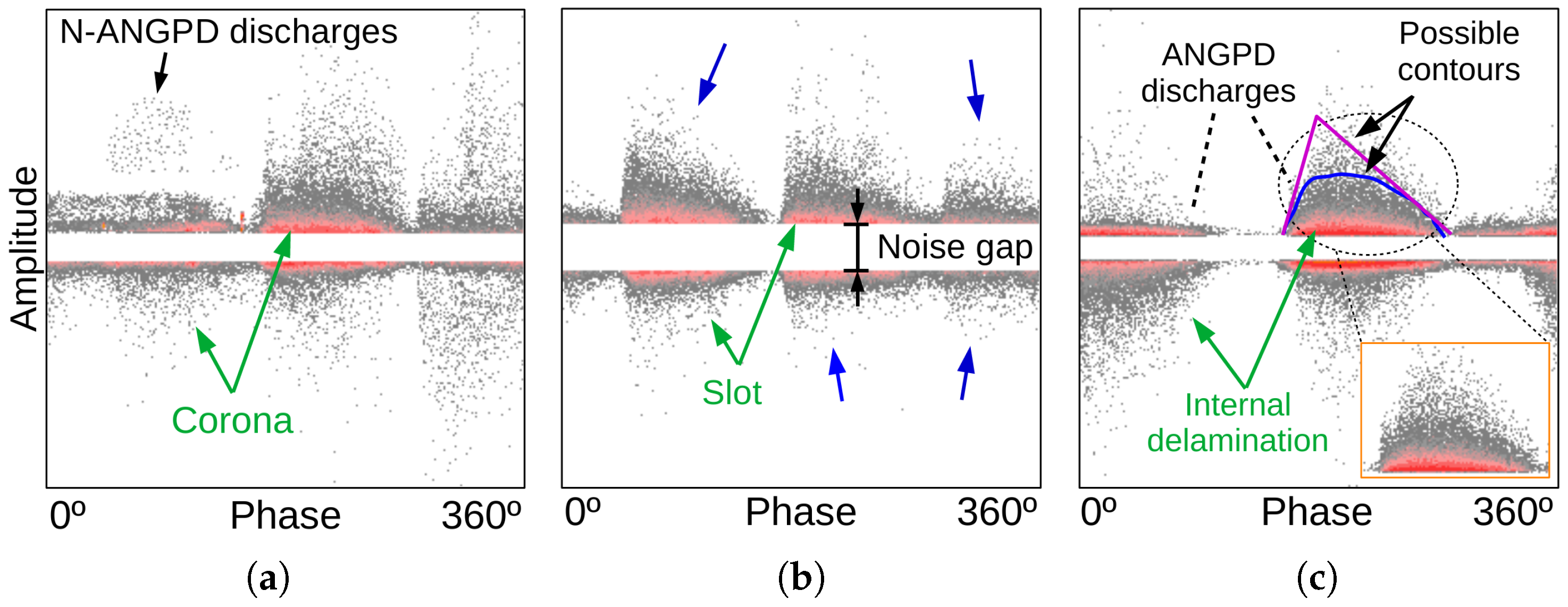
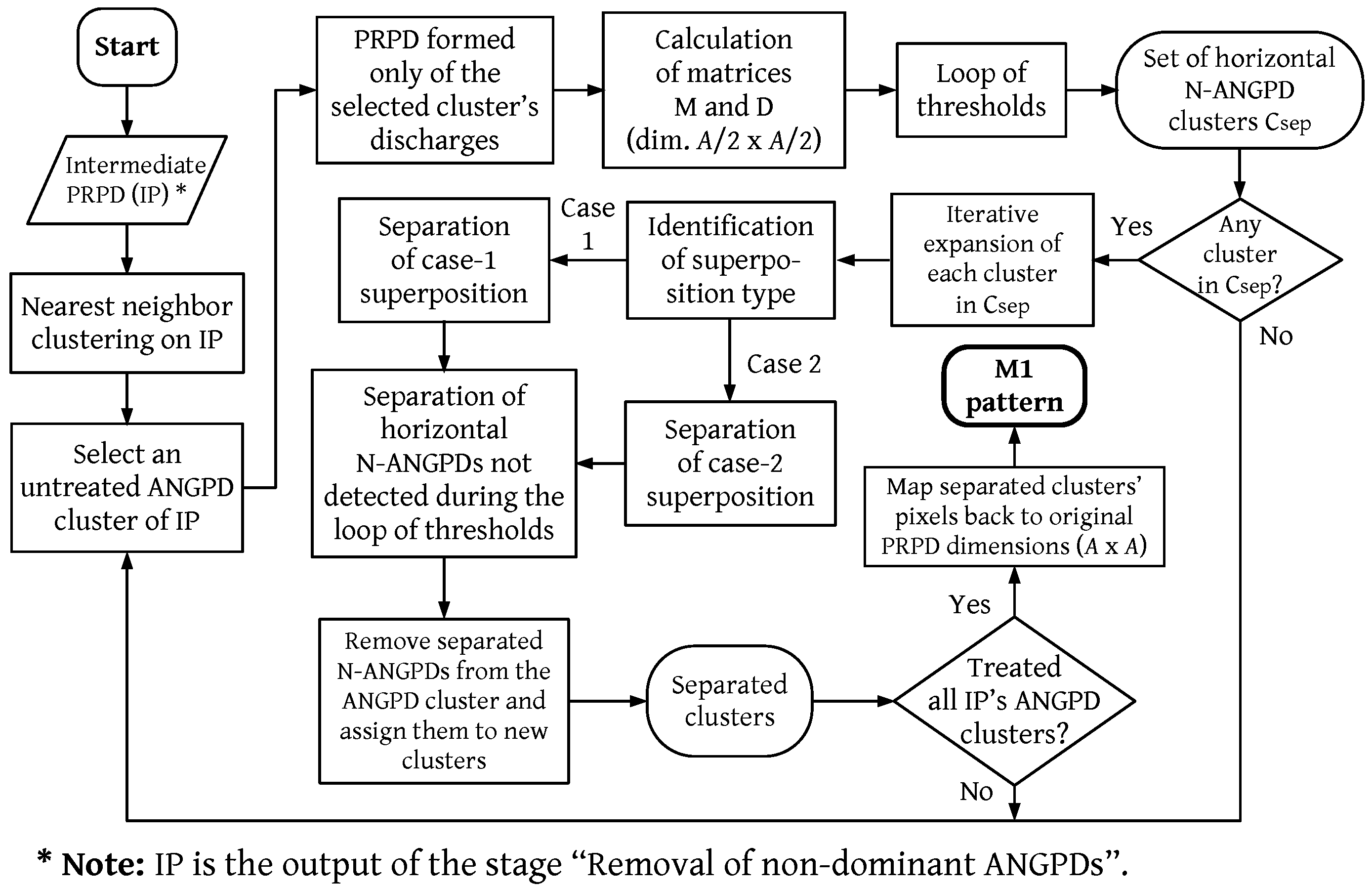
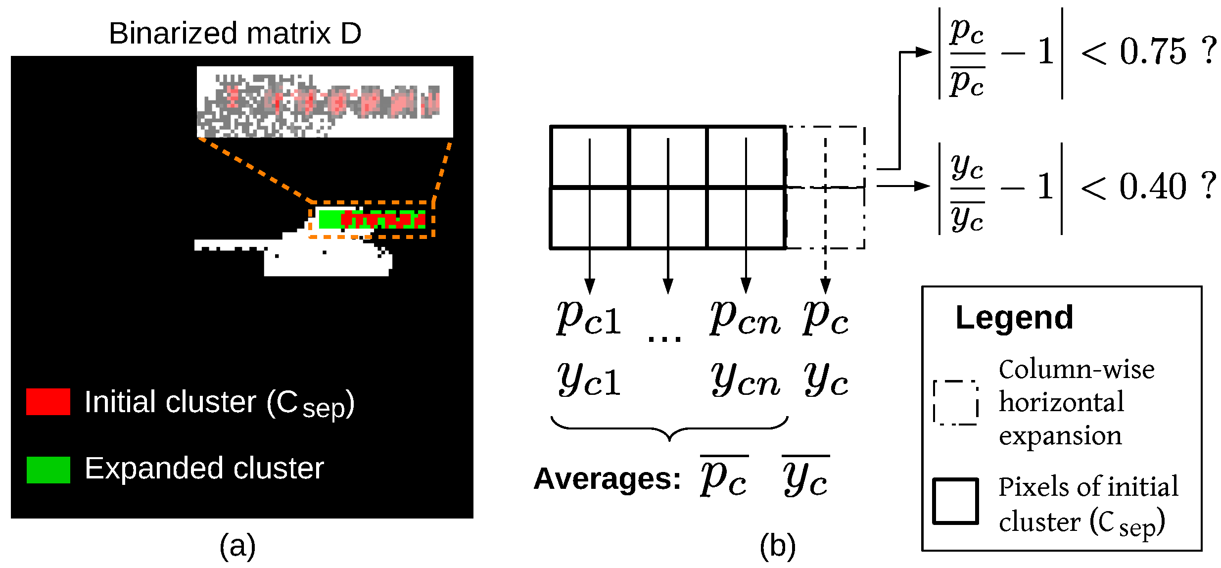
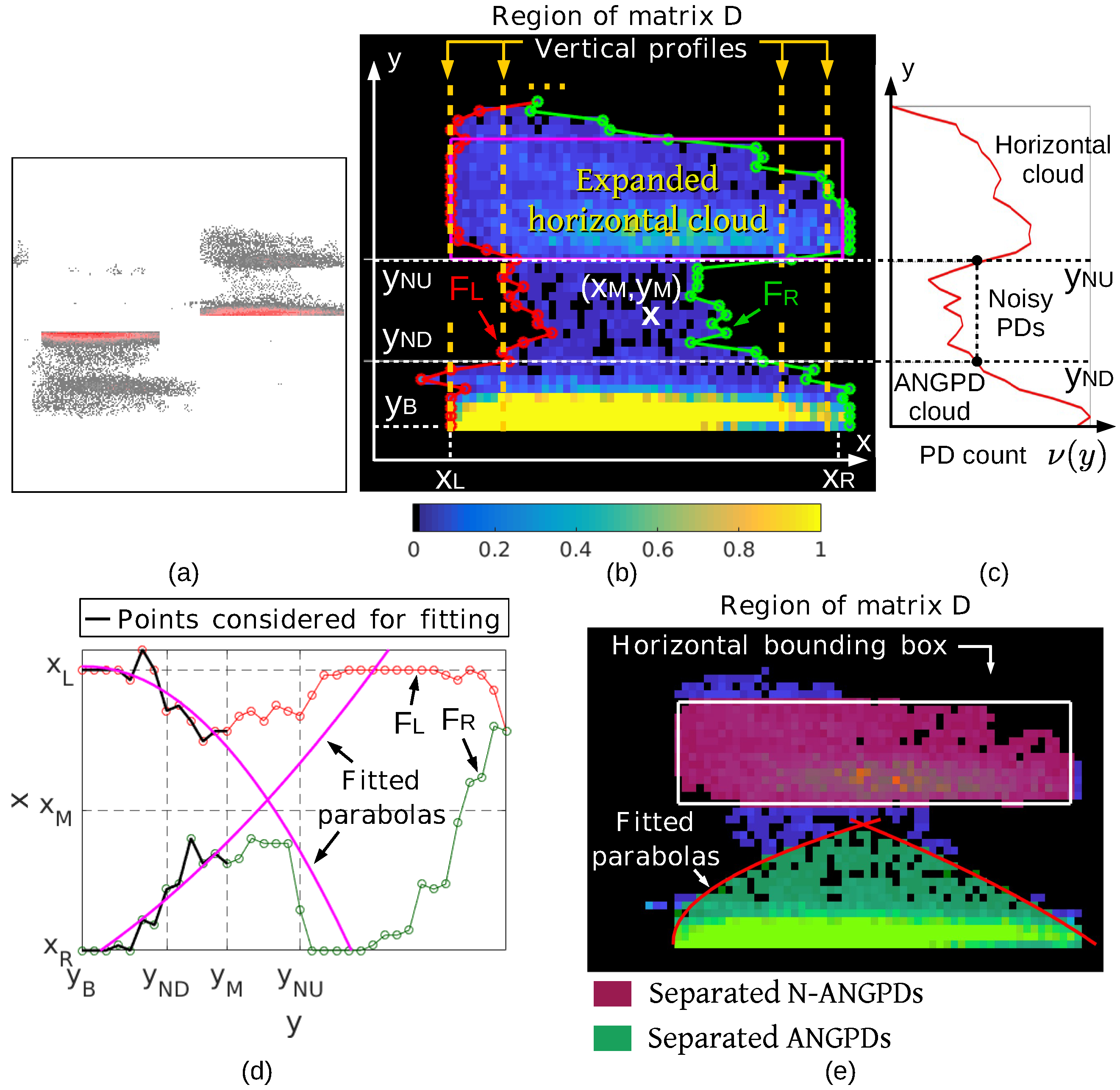
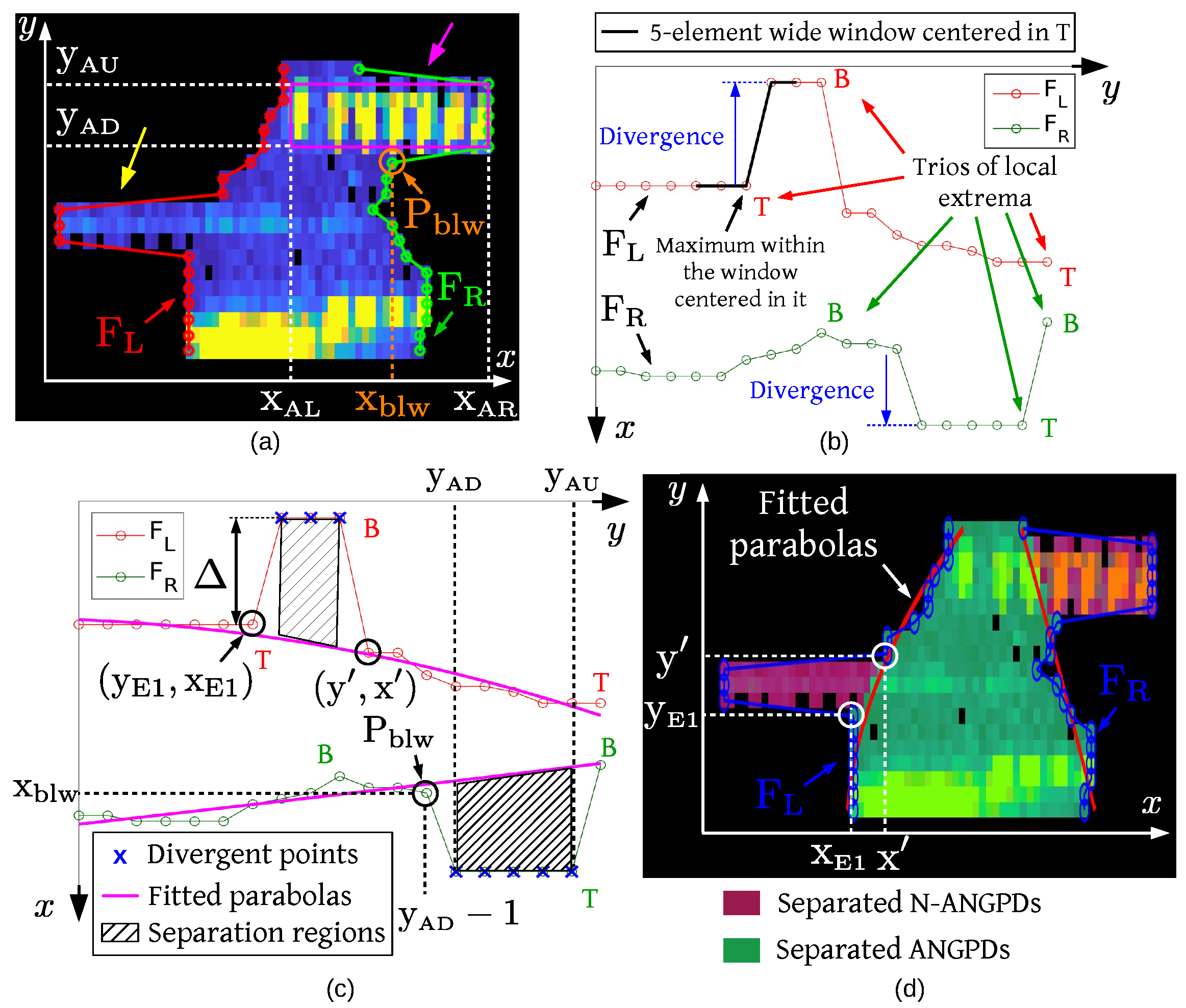
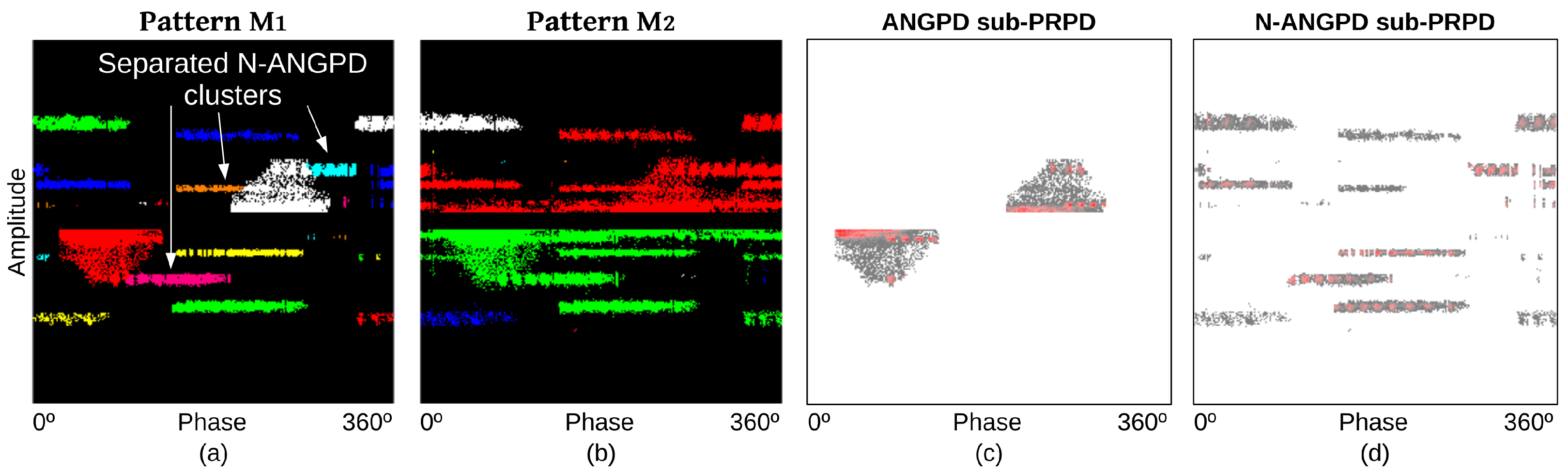
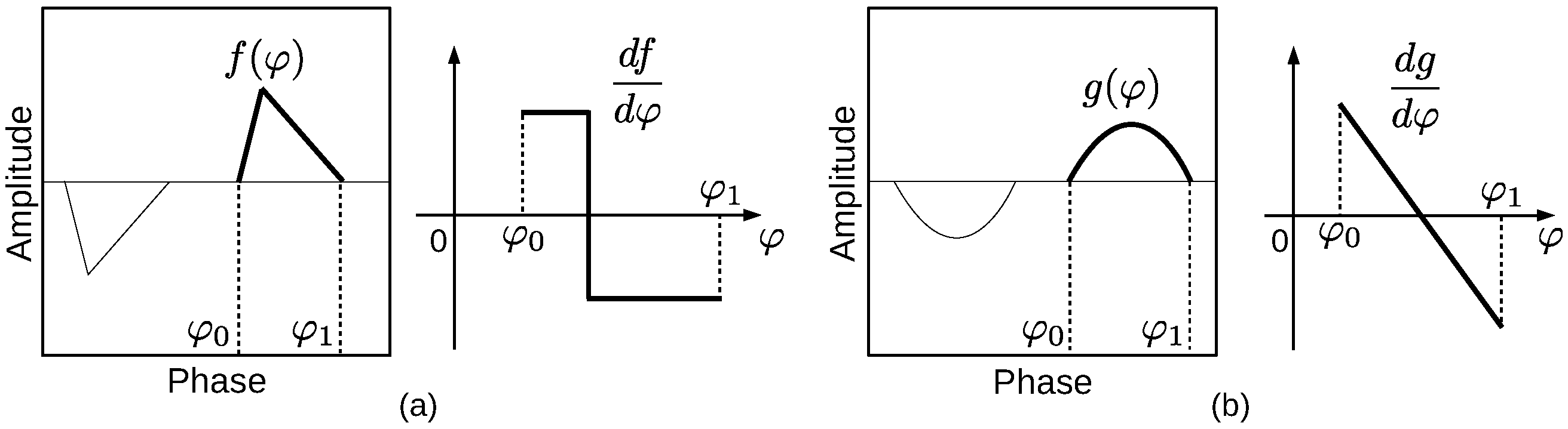
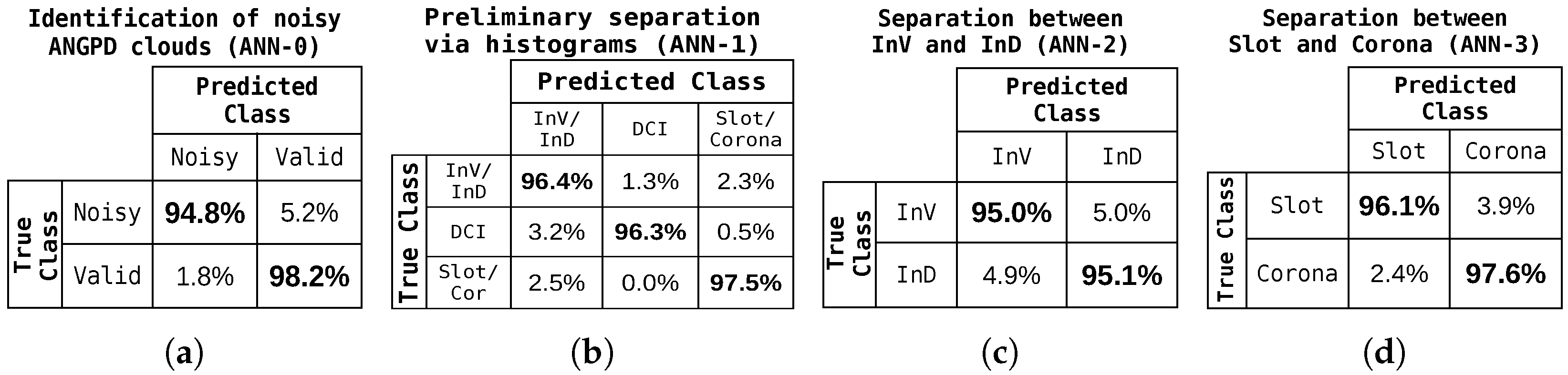
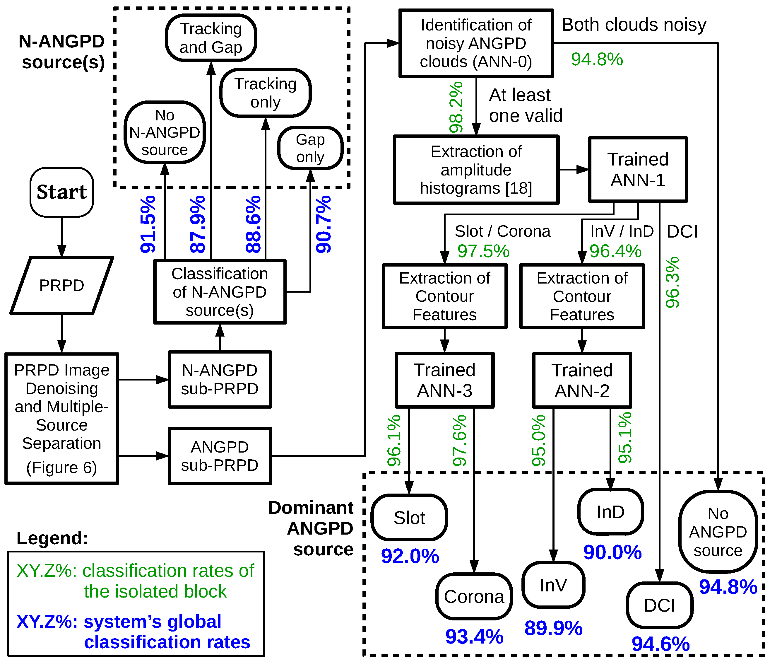
| PD Source | Symmetry between Positive and Negative PDs | Shape of PD Clouds |
|---|---|---|
| InV | Symmetric | Rounded |
| InD | Triangular | |
| DCI | Higher-amplitude negative PDs | Not applicable |
| Slot | Higher-amplitude | Triangular |
| Corona | positive PDs | Rounded |
| Tracking | Not applicable | Vertical N-ANGPD clouds |
| Gap | Pair of horizontal N-ANGPD clouds |
Table 2.
Information about the types of neural networks used.
| Property | Type of Neural Network | |||
|---|---|---|---|---|
| ANNs-0 | ANNs-1 | ANNs-2 | ANNs-3 | |
| Number of input neurons | 6 | 32 | 32 | 32 |
| Number of output neurons | 2 | 3 | 2 | 2 |
| Activation functions | Hyperbolic tangent in the hidden layers; softmax in the output layer | |||
| Size of training/valida- tion/test sets | 2430/810/ 809 | 195/66/ 66 | 51/18/ 17 | 102/35/ 34 |
Table 3.
System classification results on the patterns of Figure 3.
Table 3.
System classification results on the patterns of Figure 3.
| Pattern | True PD Source(s) | System’s Predicted Class(es) | Numerical Outputs of Internal Networks | |||
|---|---|---|---|---|---|---|
| ANN-0 * | ANN-1 | 2ANN-2 | 2ANN-3 | |||
| Figure 3a | Corona | Corona | 0.01|0.99 | 0.01|0|0.99 | — | 0.14|0.86 |
| Figure 3b | Slot | Slot | 0.01|0.99 | 0|0|1 | — | 0.99|0.01 |
| Figure 3c | InD | InD | 0|1 | 0.91|0.04|0.05 | 0.01|0.99 | — |
| Figure 3d | InV + Gap | InV + Gap | 0.01|0.99 | 0.9|0.05|0.05 | 1|0 | — |
| Figure 3e | DCI + Gap | DCI + Gap | 0.05|0.95 | 0.01|0.99|0 | — | — |
| Figure 3f | Und | Und | 0.99|0.01 | — | — | — |
* Values of output neurons associated to Noisy|Valid classes. Values of output neurons associated to (InV/InD)|DCI|(Slot/Corona) classes. Values of output neurons associated to InV|InD classes. Values of output neurons associated to Slot|Corona classes.
Publisher’s Note: MDPI stays neutral with regard to jurisdictional claims in published maps and institutional affiliations. |
© 2022 by the authors. Licensee MDPI, Basel, Switzerland. This article is an open access article distributed under the terms and conditions of the Creative Commons Attribution (CC BY) license (https://creativecommons.org/licenses/by/4.0/).
Share and Cite
MDPI and ACS Style
Araújo, R.C.F.; de Oliveira, R.M.S.; Barros, F.J.B. Automatic PRPD Image Recognition of Multiple Simultaneous Partial Discharge Sources in On-Line Hydro-Generator Stator Bars. Energies 2022, 15, 326. https://doi.org/10.3390/en15010326
AMA Style
Araújo RCF, de Oliveira RMS, Barros FJB. Automatic PRPD Image Recognition of Multiple Simultaneous Partial Discharge Sources in On-Line Hydro-Generator Stator Bars. Energies. 2022; 15(1):326. https://doi.org/10.3390/en15010326
Chicago/Turabian StyleAraújo, Ramon C. F., Rodrigo M. S. de Oliveira, and Fabrício J. B. Barros. 2022. "Automatic PRPD Image Recognition of Multiple Simultaneous Partial Discharge Sources in On-Line Hydro-Generator Stator Bars" Energies 15, no. 1: 326. https://doi.org/10.3390/en15010326
Note that from the first issue of 2016, this journal uses article numbers instead of page numbers. See further details here.