
Discrete Wavelet Transform for the Real-Time Smoothing of Wind Turbine Power Using Li-Ion Batteries
by
 , and
, and
Andrea Mannelli
1, 
Francesco Papi
1 ,
,
George Pechlivanoglou
2,
Giovanni Ferrara
1 and
Alessandro Bianchini
1,*
1
Department of Industrial Engineering, Università Degli Studi di Firenze, Via di Santa Marta 3, 50139 Firenze, Italy
2
Eunice Energy Group, 29, Vas. Sofias Ave, 10674 Athens, Greece
*
Author to whom correspondence should be addressed.
Energies 2021, 14(8), 2184; https://doi.org/10.3390/en14082184
Submission received: 29 January 2021
/
Revised: 7 April 2021
/
Accepted: 12 April 2021
/
Published: 14 April 2021
(This article belongs to the Special Issue Power Quality of Renewable Energy Source Systems)
Abstract
:Energy Storage Systems (EES) are key to further increase the penetration in energy grids of intermittent renewable energy sources, such as wind, by smoothing out power fluctuations. In order this to be economically feasible; however, the ESS need to be sized correctly and managed efficiently. In the study, the use of discrete wavelet transform (Daubechies Db4) to decompose the power output of utility-scale wind turbines into high and low-frequency components, with the objective of smoothing wind turbine power output, is discussed and applied to four-year Supervisory Control And Data Acquisition (SCADA) real data from multi-MW, on-shore wind turbines provided by the industrial partner. Two main research requests were tackled: first, the effectiveness of the discrete wavelet transform for the correct sizing and management of the battery (Li-Ion type) storage was assessed in comparison to more traditional approaches such as a simple moving average and a direct use of the battery in response to excessive power fluctuations. The performance of different storage designs was compared, in terms of abatement of ramp rate violations, depending on the power smoothing technique applied. Results show that the wavelet transform leads to a more efficient battery use, characterized by lower variation of the averaged state-of-charge, and in turn to the need for a lower battery capacity, which can be translated into a cost reduction (up to −28%). The second research objective was to prove that the wavelet-based power smoothing technique has superior performance for the real-time control of a wind park. To this end, a simple procedure is proposed to generate a suitable moving window centered on the actual sample in which the wavelet transform can be applied. The power-smoothing performance of the method was tested on the same time series data, showing again that the discrete wavelet transform represents a superior solution in comparison to conventional approaches.

1. Introduction
Wind energy is one of the most environmental-friendly and promising renewable energy sources. The intermittent nature of the wind, however, sets limits on a large-scale penetration into the electricity grid [1,2]. In fact, the variability of the wind resource can create grid instability issues, in terms of frequency and voltage. In addition, random fluctuations of wind power, if not properly regulated, may lead to the risk of undesired curtailment [3]. Therefore, in order to prevent possible damages, the requirements of the electrical system are very restrictive, constraining the power gradients that the network can absorb, as discussed in more detail in the following. This has led to the development of power smoothing approaches, i.e., methods capable of mitigating fluctuations, smoothing the power profile fed into the network [4]. Approaches without Energy Storage Systems (ESS) are becoming popular due to their low upfront investment cost, but are not mature for widespread application [5]. Studies are mainly focused on inertia control approach and pitch angle approach: the first needs a Maximum Power Point Tracking (MPPT) controller so that the rotor of the turbine can store the designated amount of energy, whilst the second is characterized by a sluggish and oscillatory response of the system [6]. However, most of smoothing techniques make use of storage systems [7,8]. Energy storages can supply more flexibility and balancing to the grid, providing grid stability and a back-up to intermittent renewable energy, but their economic impact is often not negligible. Intense research is carried out especially in developing efficient control strategies to manage the power exchange between wind turbines and storage system [9,10]. Various ESS such as superconducting magnetic energy systems (SMES), flywheel energy storage systems (FESS) [11,12], energy capacitor systems (ECS), battery storage (BESS) [13,14], and fuel cell and electrolyzer hybrid systems (FC/ELZ) [15] have been utilized to smooth the output power fluctuations and to enhance the power quality, as well as hybrid energy storage systems (HESS), combining the technologies mentioned above [16]. Lithium-ion (Li-Ion) batteries, in particular, are a mature, efficient, and reliable technology and the specific power and energy characteristics make them suitable for this type of application. Although not investigated in this study, these benefits are even more interesting if a possible reuse of batteries from electric vehicles with acceptable degradation is considered [17,18].
Several power smoothing approaches using BESS have been proposed as discussed in the review by Kasem et al. [15]. In particular, the idea of analyzing the wind power output like a signal and smoothing out the highest frequency components is becoming one of the most investigated trends. In this perspective, the application of the discrete wavelet transform (DWT) is particularly appreciated (e.g., [19]). This approach acts similar to the ubiquitous Fast Fourier Transform for time signals, even though the transformation is made in the wavelet domain, i.e., according to a prescribed shape for the signal. Beyond the specific mathematics beyond the method, that will be presented in the following Section 3.1, the key point of this method is that it can process non-stationary signals using a multi-resolution analysis [20]. More specifically, for the purpose of power smoothing, it allows to distinguish effectively within the signal those lower-frequency fluctuations that can be delivered to the grid from the higher-frequency ones that need to be compensated with a storage, as shown recently by [21,22,23].
1.1. Objectives and Novel Contributions
This study is aimed at tackling two main research requests. First, to demonstrate that the discrete wavelet transform guarantees a more effective sizing and use of the battery storage in comparison to more traditional approaches such as a simple moving average or a direct use of the battery in response to excessive power fluctuations. Benefits are quantified in economic terms, i.e., minimizing the cost of the Li-Ion battery pack for a given smoothing target. Second, the study aims at extensively testing the capabilities of the discrete wavelet transform when embedded into a real-time control algorithm that can be used for controlling the system. A simple mathematical method to generate a symmetric window centered on the current time-step is proposed, so that the wavelet transform can be performed instantaneously. A sensitivity analysis on the needed settings in terms of needed datapoints is also provided. The benefits provided by the use of the online wavelet are once again compared with conventional techniques.
The two objectives were achieved also thanks to the possibility of training and testing the developed methods on the real power output of two modern wind turbines in operation for more than four years. In comparison to other work, where the available data sets are often limited to shorter periods or even to synthetized time series, this allowed to specifically tune the discrete wavelet transform for hybrid systems including wind turbines and batteries, e.g., defining the most suitable decomposition level as a function of the required Abatement Ratio. If on the one hand real data do ensure a high level of significance of the results, on the other hand one should note that the proposed method is of more general validity and it can be easily replicated in the preliminary design phase of an industrial storage system by replacing real power time series with virtual data coming from a combination of synthetic wind time series with the turbine power curve, as many state-of-the-art siting pieces of software do.
1.2. Organization of the Study
General requirements regarding the smoothness of the power output required for wind farms are first given in Section 2. The study case is also presented in this section, coupled with a discussion on the wind data monitoring systems and a thorough analysis of the data used for the present study with respect to common grid-code constraints. In Section 3, the wavelet approach is discussed, and a battery model that considers cyclic degradation is implemented. The wavelet-based power smoothing algorithm is then described, and used for both sizing the storage system and controlling the EES in real time. The results of both approaches are finally reported and discussed in Section 4.
2. Case Study
This section presents the framework this study has been conducted into, in terms of both power smoothing requirements (Section 2.1) and selected test case (Section 2.2).
2.1. Grid Code Requirements
Even though no general requirements can be highlighted worldwide, since the electrical grids still differ significantly from country to country, a paradigm for prescribing such constraints is emerging. In particular, reference is commonly made to the “ramp rate” (RR), defined in Equation (1), to impose a limitation to the maximum speed by which the active power can vary in the case of fluctuating resources, like wind. Going into the details of the RR formulation, one can notice that a ramp event occurs when the power fluctuation ∆P(t) occurring during a given time ∆t, exceeds a threshold [24]:
The ramp rate is usually defined over periods of one minute or 10 min. Often the difference ΔP is normalized with respect to the wind plant’s nominal power Pnom. of the power plant [25]:
The typical ramp requirement is 10% of rated power per minute, but each national grid typically has its own regulation. Table 1 reports the maximum ramp rate specifications of some countries [4,15,19,26,27,28]. Upon examination of the table, ramp-rate limits vary greatly from country to country and are typically more stringent for weaker grids. Constraints on single wind turbine power fluctuations are often not this restrictive for modern electrical systems. This is due to the fact that there is spatial smoothing of aggregate wind energy generation because multiple plants in a certain region likely experience different wind speed time-series, which in practice reduces the aggregated variability [29].
Based on the comparative nature of the present study, a ramp-rate of 10% per minute is used in this study, regardless of wind farm capacity, as this is a recurrent constraint on many grids, even in case of those with high installed wind capacity, as the USA.
2.2. Case Study
One of the main points of strength of the present study is the possibility of basing the analysis on real wind turbine data collected in the field. In fact, thanks to the courtesy of EUNICE ENERGY GROUP (EEG), the authors had access to 48-months real data from two multi-MW onshore wind turbines (WTs) installed in a wind park of EEG located at a complex terrain region on the Greek mainland (Figure 1), which is in operation since 2011. The use of data from turbines operating in a complex terrain is thought of particular relevance for the study, since storage systems could be largely effective in this type of application, where gustiness and non-uniform wind field are more likely.
As a first step, the Supervisory Control And Data Acquisition (SCADA) data was analyzed in detail and properly purged of those values that do not correspond to normal operation of the turbine (e.g., maintenance periods, acquisition system errors, lightening, icing, etc.). This led to the definition of a reliable and coherent data set in the form of turbine power as a function of time and wind speed for both the turbines under investigation (see Figure 2). Please note that power data in Figure 2 and in the rest of the study are presented in a non-dimensional form (i.e., divided by the nominal power) to preserve the non-disclosure agreement with the industrial partner.
As a second step, a refinement of temporal series was needed. In fact, one should remember that in the common industrial practice SCADA data are commonly acquired with a timestep of 10 min; the typical ramp rate required by network protocols, however, is defined as 10% of rated power capacity per minute. Since standard deviations of power data inside each 10-min bin were not available, 1-min resolution data were generated a posteriori by means of a properly tuned random function. The function extracts, for each 10-min bin, 9 values in the range between the maximum and the minimum power as reported by the SCADA (so that no wind speed could be introduced that was not present in reality), while the 10th value is the mean power on that period. The high-resolution power time series maintains the same Annual Energy Production that would be calculated using the original SCADA data; in other words, the random values were selected so that the energy produced in the 10 min bin is equal to the sum of the energy produced each 1-min bin in the same period. An example of the outcomes of the procedure is shown in Figure 3a,b. Ideally, it would have been preferable to use real 1-min data over this energy-conservative extrapolated data. However, this approach is arguably conservative with respect to battery sizing requirements as it is highly unlikely that the wind speed, and thus the output power, will follow a completely random pattern in the sub 10-min window [4].
Analyzing the data in further detail, Probability Density Functions (PDF, in Figure 4) and Cumulative Density Functions (CDF, in Figure 5) were used to highlight the distribution of ramp rates occurrence. Upon examination of the CDF, it is apparent that, as expected, most of the ramp rates are under the regulation threshold; in particular, over 20% of the cases are over the 10% limit in the 1-min data series, which is a considerable amount. Smoothing all the ramp rates might require a very large battery capacity, which could make a project economically not convenient. As it is often the case in the field of engineering, the solution to the problem might be a tradeoff between multiple objectives, i.e., smoothing effectiveness and battery size in the present application. This is the reason why the effectiveness and the costs of the power smoothing system will be evaluated in terms of abatement ratio (AR), defined as [4]:
AR is equal to 1 if all the ramp-rate violations are smoothed, while it gets lower and lower as the ESS falls behind and is unable to absorb the power surplus from the power plant. Rather than simply describing the percentage of fluctuations that violate the ramp-rate limits, this parameter quantifies the percentage of fluctuations, which violated the constraints in the un-smoothed signal, which have been removed in the smoothed one. By defining this parameter, a storage system that maximizes AR while keeping costs reasonable can be selected.
3. Methodology
The following section will describe the methods and related algorithms used in the study. A theoretical overview of the Wavelet transform is discussed, followed by a detailed overview of the implemented smoothing method, with special focus on the proposed method for using DWT online. The conventional methods against which the proposed smoothing algorithm is benchmarked are also discussed. In addition, the methods for battery sizing, operation, and aging are presented.
3.1. Discrete-Wavelet Based Signal Approximation
The Discrete Wavelet transform (DWT) was selected as the most promising power smoothing technique to be investigated for the scopes of the present study. Generally speaking, the Wavelet transform can be seen as an analysis tool for extracting local-frequency information from a non-stationary signal [31]. A complete overview on the mathematical formulation of the method is beyond the scope of the present study and does not represent an original contribution. However, to convey the basic elements needed to understand the developed algorithm, a brief dissertation on the wavelet theory is here reported. For more information, the reader could refer to refs. [32,33,34,35,36,37,38] which were used for this discussion.
In signal processing, the most popular technique is the ubiquitous Fourier Transform (FT), i.e., the definition of the amplitude of all the frequency components that, summed together as correspondent sinusoidal waves, are able to reproduce the original signal. The problem of the FT is, however, represented by the fact that no indication about the exact time in which each frequency gave its contribution is provided. In case of a stationary problems, this is not a particular issue, as the properties of the signal are maintained over time in a recurring way. On the other hand, when the signal is not stationary, like a wind power time series, the most straightforward option is to modify the approach by representing the signal in two dimensions, i.e., with time and frequency coordinates. To do so, one small signal section (defined by a window function) is analyzed time by time; assuming the stationarity of the signal inside this window, the Fourier transform is applied section by section, sliding the window along the signal. This method is usually called Short-Time Fourier Transform (STFT) and it can provide more specific information about the location of the different frequency components. On the other hand, its accuracy is intrinsically affected by the selection of the signal-cutting window, which can be well explained by Heisenberg’s uncertainty principle applied to signal processing, stating that one cannot identify correctly at the same time the frequency and the time of occurrence of this frequency. Mathematically, this can be expressed in terms of standard deviations of the time and frequency as follows:
Based on Equation (4), one can readily notice that, defining a certain level of accuracy in time or frequency with the choice of window size, the other follows accordingly.
Moving from this background, particular attention is currently given to the use of Wavelet analysis, since it implies a windowing technique with modulated windows able to mitigate or suppress the signal-cutting problem. In further detail, wavelet functions are defined conventionally as wave-like oscillations of finite amplitude that have null average [35]. Wavelet have the advantage that they can be manipulated either by sliding them along the signal or by varying their extension. In other words, the wavelet approach can be seen as a windowing technique with variable-size regions. it allows using long time intervals where more precise low-frequency information is required, while short time intervals are used where more precise high-frequency information is required. By doing so, the wavelet transform allows the variation of and at different frequencies, without violating the uncertainty principle and thus allowing for both a correct definition of the frequency content in the signal and their location in the time domain: this kind of approach is defined multiresolution analysis (MRA).
Many different shapes of the wavelet function are available, usually referred to as mother wavelet [38]. The extension of the wavelet is governed by the scale factor a, while the movement along the time axis is described by the translation factor b (Equation (5)). By translating and scaling the mother wavelet shape, it is possible to obtain an infinite number of wavelets , identified by parameters and and defined as follows:
where the term is used to normalize the wavelet.
The theoretical aspects, described in the previous introductive part, bring to define the continuous wavelet transform (CWT) for a signal by adopting a mother wavelet function which is properly written as:
where the superscript ∗ denotes the complex conjugate.
The inverse wavelet transform can be defined in the following form:
where the term is the admissibility constant and its value depends on the chosen wavelet. For more information, please refer to [34]. It is worth pointing out here, however, that in terms of applicability CWT has three main issues:
- Redundancy, since CWT is defined as a continuous integral, affecting considerably the calculation time;
- CWT is defined on an infinite number of wavelets identified by the scale and translation factors, which can assume infinite values;
- For most of the functions the wavelet transforms have no analytical solutions, and they can be calculated only numerically.
In order to make CWT more practical and easily applicable to engineering problems, the Discrete Wavelet Transform (DWT) is introduced. To remove the redundancy, DWT considers only discrete values of the scale and translation factors. The wavelet is discretized by a logarithmic discretization of the scale parameter . The size of the steps taken between locations is correlated to the scale parameter by proportionality. The discretized wavelet therefore takes the following form (Equation (8)):
being m and n integers that control the wavelet dilation and translation, respectively. More precisely, different m values correspond to wavelet of different widths. The value of the translation parameter depends on the width of the wavelet: narrower wavelets will be translated with a smaller step to cover the entire signal extension; wider wavelets, on the other hand, will have a larger step. Commonly, for practical reasons and are chosen equal to 2 and 1 respectively, so that the samplings of both the frequency axis and the time axis correspond to dyadic samplings. A dyadic grid is the most efficient discretization for practical purpose and allows the construction of an orthonormal wavelet basis.
With the removal of redundancy, the second goal is to reduce the number of wavelets needed in the wavelet transform, which is still infinite. In the Fourier analysis, the spectrum of the signal is dilated and moved to higher frequencies, as consequence of a time compression. Similarly, a wavelet compression of a factor 2 will bring to a spectrum expansion by the same factor and a frequency shifting upwards. Otherwise, the wavelet spectrum is halved as a result of a doubling of its width in the time domain [37]. Since a wavelet can be seen in first approximation as a band-pass filter, this last aspect leads to a halving of the bandwidth. By exploiting this property, it is, therefore, possible to cover the signal spectrum with the wavelet spectra of different extensions. A good coverage can be obtained if the spectra associated with the wavelets of different scales are connected, without leaving any gap. This process, however, would require an infinite number of wavelets of different scales to cover the entire signal spectrum down to zero frequencies. It is therefore necessary to introduce a new element of the wavelet analysis, which is the scaling function. The scaling function is associated with the smoothing of the signal and its spectrum has the nature of a low-pass filter. Mathematically, the scaling function has the same form of the wavelet: that is,
and it satisfies the following property:
where is called father scaling function or father wavelet. By introducing the scaling function, the problem of the infinite number of wavelets has been resolved setting a lower bound for the wavelets. In this way, one wavelet is analogous to a band-pass filter and a scaling function is a low-pass filter and, consequently, a series of dilated wavelets together with a scaling function is a filter bank.
Finally, for resolving the third issue of CWT, fast algorithms to calculate the wavelet transform must be developed. The most efficient way in terms of calculation time is to divide the signal spectrum in two (equal) parts, i.e., a low-pass and a high-pass frequency band. The high-pass band includes the smallest details, while the low-pass part still contains some information and therefore it is possible to split it again, creating an iterated filter bank. The number of bands is limited by for example the amount of data or computation power available. The advantage of this scheme is that we must design only two filters, while the disadvantage is that the signal spectrum coverage is fixed. A more detailed dissertation on the frequency range characterization related to the wavelet transform is present in [39].
Ultimately, as in many practical applications signals are discrete, described wavelet transforms must also be discretized. In fact, discrete wavelets are not time-discrete but only the translation and the scale step are discrete. To achieve the time-discretization, the wavelet filter bank can be implemented as a digital filter bank. This brings to define wavelet families through two filter banks: the scaling filter and the wavelet filter. This last procedure can be seen in analogy with the Fast Fourier Transform as reported in [40].
In order to clarify this process, Figure 6 shows the application of DWT on a small sample of the original wind power signal of the present case of study. As discussed, the scope is to decompose the wind power into high-frequency and low-frequency components. Discrete wavelet transform returns two sets of coefficients: approximation coefficients (in red in Figure 6) and detail coefficients (in green in Figure 6), which represent the output of the low pass filter (averaging filter) and high pass filter (difference filter), respectively. Then, DWT is applied iteratively on the low pass set, so that the original signal is also sampled down by a factor of 2. The process is shown in Figure 6a. In this way, it is possible to analyze in the signal at different frequency levels reaching the required degree of decomposition. Once the wavelet coefficients are calculated, the inverse discrete wavelet transform is applied to each level separately to reconstruct a power signal filtered from the high-frequency components (Equation (11), where n is the level of decomposition selected). The wavelet decomposition diagram of wind power is shown in Figure 7, where A and D represent the low frequency and the high frequency components of the signal, respectively.
As a final remark, it is worth noting that, to ensure an accurate signal reconstruction, an appropriate choice of the most suitable mother wavelet must be made. In fact, the best wavelet to perform the analysis depends on the type of signal and the phenomenon of interest [21]. In this study, the Daubechies Db4 has been selected as mother wavelet because of its specific properties, i.e., orthogonality, energy preservation and support of higher polynomials grade for the same number of vanishing moments in comparison with other families, in accordance with literature results [41]. In particular, the Daubechies wavelet Db4 offers an appropriate trade-off between wavelength and smoothness, resulting in an optimal behavior for wind power smoothing and short-term wind power forecasting.
3.2. Wavelet-Based Smoothing Algorithm and ESS Model
The DWT is at the core of the proposed smoothing method. The signal is first decomposed into a low frequency component that will be outputted to the grid and a high frequency one that will be absorbed by the ESS. This concept remains the same in both the battery sizing algorithm, presented in Section 3.2.1 and the battery management algorithm, shown in Section 3.2.2. The constraints on the ESS’s operation are at times a significant bottleneck and cause the power output to the grid to change significantly. For this reason, the ESS and the smoothing algorithm have to be treated as a single system as will be explained in the following subsections.
3.2.1. DWT-Based Battery Operation Design Algorithm
The wavelet-based analysis is applied to the smoothing of a wind turbine’s power output by firstly decomposing the signal into low and high frequency components. This section in focused on the description of the algorithm used for batter sizing. Therefore, the DWT is performed on the entire dataset at once. The flowchart in Figure 8 describes the logic of the algorithm. The inputs of the model are shown in Table 2. All the algorithms developed in the study were realized in the Python programming language. As shown in Figure 8, once the input data is acquired, the DWT is performed, and the recursive part of the algorithm begins and the procedure cycles through all the timesteps of the input data.
After the DWT of the power signal is calculated, the target smoothed power output is reconstructed considering the frequency threshold given by the selected level of decomposition. A higher level of wavelet decomposition will smooth out a larger portion of the signal, while a lower level will filter out fewer high frequency components. Possible negative values of the low-frequency component have also to be checked as they are physically wrong: these values are set equal to zero. Subsequently, a first use of the battery is made: a positive smoothing involves a discharge of the battery while a negative smoothing entails a charge of the battery as illustrated in Figure 9.
The smoothed power resulted by the DWT is then checked for ramp rate violations. If no violation occurs, the power output is equal to the power smoothed by the DWT, and battery parameters are updated before the next timestep. If a ramp rate violation takes place, an additional smoothing step is required. It is readily noticeable that the algorithm needs to work in tight connection with the battery model as the battery is required to absorb the excess power, which can be easily computed as:
To model real-world operation some constraints regarding the battery have to be introduced and will be detailed in the following section.
3.2.2. DWT-Based Real-Time Battery Control
The Discrete Wavelet Transform is typically used in many engineering applications for the analysis of acquired signals; this kind of approach perfectly fits the application where it is used to properly size a storage system based on either historic data, like those available in this study, or synthesized ones.
On the other hand, the present study aims at showing this method can be exploited for performing power smoothing in real time. To this end, however, the conventional method needs to be re-arranged. More specifically, it is commonly acknowledged that DWT exhibits problems of border distortion [42], i.e., inaccurate signal reconstruction is expected at the tails of the data fed to the DWT. This is of course an issue in a real-time application, where the value that needs to be handled at each timestep is exactly the last one in the series, without any future knowledge of the signal, placing the point of interest on the edge of the signal to be smoothed.
A simple and efficient approach to reduce signal discontinuities is the use of a symmetric extension method has been recently proposed in [43] and further expanded in the present study. In detail, if the goal is to calculate the real-time DWT of the signal in at certain time i, good results can be achieved by applying the DWT to a mowing window W_i symmetrically extended as follows:
In other words, the signal upon which the DWT will be performed is made of lw values before time i and ls mirrored values with respect to time i. Since the DWT is applied on a moving window of length lw+ls at each timestep, the choice of the lengths ls and lw becomes fundamental to reach high accuracy and acceptable computation time, especially important for an online tool. Considering the DWT implementation and operation as explained in [44,45], the required length of the symmetric window increases with the rise of the decomposition level, and also depends on the mother wavelet function itself. In addition, as it will be shown clearly in Section 4.5, increasing lw over a certain point does not add any information for the definition of the real-time value at the present timestep because of the multi-resolution properties (in time and frequency) of the wavelet transform. Indeed, unlike the Fourier transform, the wavelet analysis acts only close to the chosen timestep, with a range defined by the wavelet family features and decomposition level [31]. From another perspective, when increasing the level of decomposition, lower frequencies need to be approximated using the DWT, and therefore a longer window is needed. This proposed real-time method will often be referred to in the following parts of this study as “online” DWT, while when the DWT is performed on the entire dataset at once we will refer to it as “offline”.
3.2.3. ESS Model
Lithium-Ion batteries were selected as the technology to be used in the HESS because of the high efficiency and resiliency to cyclic operations in comparison to other battery technologies [46]. The dynamic behavior of the batteries is neglected as Li-ion batteries have a very fast response time (within milliseconds), much shorter than the timestep assumed in the analysis (one minute). In order to obtain more realistic results, both operating constraints and battery degradation were accounted for, since it is well known that batteries tend to reduce their available capacity due to cyclic operation. Calendar or shelf aging was not considered in this study as the battery is continuously in operation and this aging mechanism only affects battery lifetime when the component is stored at a constant state of charge for prolonged periods of time.
State of Charge (SOC) is an expression of the residual battery capacity as a percentage of maximum capacity. To prevent quick battery degradation, SOC is always somehow limited by the control system, as very deep charge-discharge cycles are particularly damaging. In this study, the allowed variation range for SOC was between 0.15 and 0.95. Other characteristics to need to be monitored are the charge and discharge currents, which have to be limited to prevent battery damage. Within the framework of the present modeling approach, where the SOC range is restricted, voltage can be considered constant, and currents can be evaluated in terms of charge and discharge power (kW). As the current magnitude depends on the battery size, the “C-rate parameter” is defined as C-rate = Power (kW)/Capacity (kWh). High C-rates generate an increase of the battery working temperature, reducing efficiency and lifetime. Therefore, precautionary constant C-rates of 1 for the charge phase and 2 for the discharge phase are used to prevent any issues related to temperature operation and losses of performance [47]. Moreover, charging and discharging operations entail significant losses, which are quantified in terms of their respective efficiencies [48]. They are relative to different parameters, such as SOC and temperature. Assuming that the latter is constant given the constraints on C-rates, a non-linear behavior of the charge/discharge efficiencies in function of the SOC is taken into consideration to model in a more accurate way the battery operation. As shown in Figure 10, because of limitations due to the electrochemical processes, discharging (spontaneous reaction) is more efficient than charging (non-spontaneous reaction) [49].
State of Health (SOH) provides an indication of the aging of a battery compared to ideal conditions. SOH values are expressed as a percentage, where 100% corresponds to a new battery and 70% corresponds to a battery that needs to be replaced in this study. This latter value is in agreement with the common prescriptions that can be found in literature (e.g., [50]). It is important to note that SOC and SOH jointly influence battery operation. The residual charge in the battery at any given time and the C-rate can be expressed as:
Therefore, as the battery ages, it might not be able to fulfill the operational requirements as both capacity and sustainable C-rates decline. The SOH of the battery is updated every 24 h accounting for battery ageing. In order to model the reduction of the maximum battery capacity caused by cyclic degradation, concepts from the field of fatigue are adapted to the present case. Battery lifetime is often estimated as the number of full charge–discharge cycles that the battery can sustain. In real-world applications however the charge–discharge profile is irregular and full cycles are rare. According to many engineering applications, the Rainflow cycle counting method is adopted to accurately identify cycles in an irregular battery SOC profile [51] and to obtain an equivalent set of constant-amplitude cycles that the battery has performed in the analyzed interval. The process is clearly explained in [52]. For each set of constant amplitude cycles the damage D caused on the battery can be calculated:
where EOL_(Cycle_m) are the maximum cycles that the battery can tolerate at the given SOC, and N_m are the cycles the battery went through at the SOC. For each SOC, the cycles the battery can tolerate can be approximated with a battery specific Wöhler curve:
The parameters A and B were estimated based on available data and literature. In particular, B = −1.5 which is a typical empirical value for this type of batteries also used by other authors in similar studies [4]. The constant A = 5200 is instead referred to the Samsung battery model with the main technical specifications reported in Table 3, being equal to the End of Life (EOL) cycle lifetime of 70%. In other words, after 5200 full cycles, the battery must be replaced because the relative capacity reaches 70% of the nominal capacity.
Considering the hypothesis of linear accumulation of damage (also known as the Palmgreen–Miner rule):
The cumulative damage gives an indication of the amount of equivalent full cycles so that it is possible to evaluate the SOH of the battery, and consequently the reduction of available capacity due to the degradation, using the function given by the interpolation of battery datasheet:
In particular, this equation derived by a second order interpolation among three points (n° cycles; SOH): (0; 100%), (3200, 80%), (5200, 70%).
It is important to notice that with the imposed limitations on C-rates and assuming controlled operating temperature, other charge or discharge power degradation mechanisms were here reasonably neglected.
3.2.4. Effects of Battery Constraints on the Wavelet Smoothing Algorithm
The effects of the introduced constraints on battery operation can now be explained. Indeed, to account for these battery-related limits, a SOC feedback strategy is a basic and important strategy to keep the SOC of BESS within its proper range while the BESS is smoothing out the fluctuations of the power signal [53]. Unlike other approaches that act directly on the SOC profiles [54], the control method developed in this study is applied directly to the wind power signal using the DWT. By doing so, the results of Section 4.2 will show that an alleviation of the battery operation stress around the SOC limits can be achieved and, by consequence, a more effective battery management. In particular, the algorithm behavior is different in charging mode (E_batt > 0) and discharging mode (E_batt < 0). Battery SOC is updated at every timestep as summarized in Table 4. The effects on power output are shown in Figure 11. Analyzing Figure 11, when the battery performance is limited by the C-rate or the SOC, the power output profile is forced to follow the red line. Therefore, depending on the battery capacity, it is possible that not all the ramp violations can be smoothed. For this reason, it is important to quantify the smoothing performance in connection with the battery capacity.
3.3. Conventional Power-Smoothing Methods for Benchmarking
In order to assess the potentiality of the proposed wavelet approach, it is here compared to two other conventional power smoothing methods. The methods are implemented similarly to the wavelet algorithm and can be conceptually illustrated as in Figure 8.
The first method is the “ramp rate shaving” approach, which directly smooths out the power when there is a ramp rate violation, i.e., the ramp rate is higher than the grid code limit. This approach does not operate a continuous smoothing, but the BESS is activated only during violation occurrences [4]. This is a simple way of providing the required smoothing, but it comes with non-negligible downsides, which will be shown in the following sections.
The other approach is the “simple moving average” (SMA) approach [55], which calculates the smooth power output at the current timestep as the average of the previous n timesteps [56]. If Pwind(i) is the wind power at the timestep i, the approach can be expressed as:
With this method, short-term averages (low n) respond quickly to changes in the power output, while long-term averages (high n) are slow to react. The battery operates continuously, storing or releasing the energy in accordance with the difference between the real wind power value and the smoothed one, predicted by the SMA. In case of ramp rate violation of the smoothed power profile, a second smoothing to respect the grid code requirement is necessary. This second smoothing is performed with the ramp rate shave method.
3.4. Cost Analysis
To the best of authors’ knowledge, no clear regulations about economic benefits and penalties associated to wind-farm violation of the ramp rate limits are in place at the time of writing, at least in European countries. As a result, no indication on fees regarding grid code violations are indicated by the literature. Therefore, the requirements reported in Table 1 are currently only recommended. According to industry insiders, however, such mechanism will arise in the near future. In order to provide a quantification of the possible benefits introduced using the wavelet method for power smoothing, the authors decided to compare the overall cost of the storage system (i.e., capital cost for batteries and maintenance cost, in the form of battery replacement [57]) with that resulting from a storage management based on the conventional methods presented in Section 4.3. While not ideal, since this study is comparative, such an analysis can still provide meaningful information.
The cost analysis is done on a 20-year time window, which is a common wind-park lifespan. According to published data, a typical battery and inverter system costs 300–350 €/kWh for large systems (>10 MWh) and 400–500 €/kWh for smaller systems [58]. In this case, considering the turbines’ rated power, a unit price of 500 €/kWh is assumed. Additionally, the cost over the period must also consider the maintenance cost and, above all, the replacement times, i.e., the substitution due to the degradation during operation. For instance, a small battery, which has to satisfy higher charge–discharge cycles, tends to age faster than a bigger one. Subsequently, the management of the battery is fundamental in order to preserve it and reduce the degradation rate. Moreover, a maximum life expectancy of 10 years is considered for precautionary reasons as most suppliers suggest [59]. The cost of the battery directly depends on the capacity. Therefore, since the battery needs to be replaced during the wind turbine’s lifetime, future capital costs need to be actualized using a discount and inflation rates. All the economic parameters are resumed in Table 5.
The cost analysis is made in a differential way. This involves assuming that revenues and maintenance costs are equal for all of the power smoothing approaches. Therefore, only differential costs have to be accounted for, these are the capital costs related to initial battery purchase and replacement. Because SCADA data is available for a 4-year period only, this data is repeated until the 20-year limit is reached. The annual cost at year n is calculated as:
The total cost over the WT lifetime is:
4. Results
4.1. Sensitivity Analysis on the Wavelet Level Decomposition and Abatement Ratio
The wavelet smoothing power profile depends on the choice of the level of decomposition. To this end, a preliminary analysis was made to assess the best level to use for the present application. The main results are reported in Figure 12, where #1 represents Level 1 (i.e., one application of the DWT on the signal). Turbine WT1 was used as a reference in the rest of study.
As expected, based on the nature of the wavelet transform, conceived to filter the high frequency components from the lower ones, it is apparent that the higher the order of the wavelet, the smoother the signal. For the limit investigated cases (levels from 1 to 7), a smoothing level equal to one does not smooth the signal (the processed signal nearly follows the raw wind power trend), whilst a level equal to seven creates a flat signal that cuts out all the fluctuations. The objective of the ESS however is not to completely level-out the turbine’s power output but rather to smooth-out the high-frequency fluctuations. To select the appropriate level of decomposition, however, battery behavior and size have to be accounted for. In fact, selecting a higher level of smoothing means that more energy must be stored or released from the battery and, therefore, a bigger battery capacity is needed to satisfy the requirements. Consequently, the selection of the wavelet level decomposition is a trade-off between the abatement ratio, i.e., the effectiveness of ramp rate reduction, and the battery capacity, i.e., the ability to follow a specific power output profile at a reasonable cost.
Figure 13 illustrates the abatement ratio as a function of the battery capacity for the seven wavelet decomposition levels discussed above. As expected, the curves present an asymptotic trend in dependency on the battery capacity, with higher-order Wavelet methods reaching smaller AR in case of small batteries, which are not able to store/release the amounts of energy needed to smooth out the original power production of the wind turbine. For the selected case study, if one sets a threshold for AR lower than 98%, the best performance (i.e., the lowest battery capacity able to guarantee such level of abatement) is given by level #2. On the other hand, if AR = 100% is requested, the Wavelet level #3 has to be preferred. Beyond the analysis of the pure frequency components that each decomposition level is able to deal with, it is also worth remembering that very high levels of decomposition not only implicate the requirement of a bigger capacity to reach a high abatement ratio, but also cause the absorbed or released theoretical power to be significant. In such cases the C-rate limits are a significant constraint and play a key role in limiting the smoothing effectiveness.
The multivariate analysis of Figure 13 showed that the choice of the decomposition level and the resulting system cost are strongly related to the selected Abatement Ratio that one wants to achieve for the system. The meaning of the AR threshold is apparent upon examination of Figure 14, which reports the PDF and CDF of the ramp rates managed by the system in case of abatement ratios of 0% and 90%, respectively.
The PDF with 90% AR is narrower than the original one because most of the ramp rates are concentrated in the range of ±10%. In particular, the CDF indicates that an abatement ratio of 90% reduces the overall ramp violations from 22% to 2%. This means that with a battery with reasonable capacity and cost, it is possible to eliminate over 90% of the ramp rate violations. In addition, no ramp-rate violations exceeding 63% rated power are recorded and even the ramp rate violations that exceed 20% are greatly reduced to a mere 1.6%.
Upon examination of the results in Figure 13, a Wavelet decomposition level of two was selected as the best compromise for the present application. As shown in figure, the optimal level of decomposition depends on the level of smoothing required, but also on the power output of the specific wind turbine or wind farm under consideration. In general, the optimal decomposition level can be determined using the proposed technique on historical data, if available. As discussed, if these latter are not available as in the case of new wind farms, synthetic power data can be derived combining anemometric measurements acquired during the wind farm planning with turbine performance curve. In addition to that, it could be possible also to find optimal level for different seasons using for example genetic algorithms as proposed in [19], but this additional study is out of scope of this paper. Furthermore, accounting for seasonal variation is not a trivial task as significant year-to-year variations can occur, and then very long time histories are needed to make the results significant.
4.2. Wavelet-Based Power Smoothing Performance against Conventional Methods
The smoothing capability of the Wavelet method (decomposition level #2) is compared to the conventional methods presented in Section 3.2. The ramp rate shave method is also targeted in the following as “Direct” approach since the smoothing is applied directly on the ramp rate violation. In addition, the optimal n for the Simple Moving Average has been selected as 20 by a sensitivity analysis. Figure 15 compares the Wavelet, the direct method, and the moving average in terms of AR vs. battery capacity. Upon examination of the figure, it is apparent that the wavelet shows by far the best performance, reaching for each battery capacity the highest abatement ratio. From another perspective, this means that, for a selected AR (e.g., 90%) the use of the Wavelet approach allows one to select the smallest battery capacity.
This result is due to the benefits associated with the analysis of the power output as a signal. Indeed, high ramp rates are directly related to high frequency components, which can be effectively located and filtered by the wavelet transform. The direct smoothing method, instead, only activates the ESS when a ramp violation occurs: this lower use of the battery potentially reduces cyclic wear but, at the same time, the intermittent operation might force the battery to provide large power and energy transients, impacting the smoothing effectiveness. The moving average approach predicts every point based on the average of a given number of previously recorded data points. This approach, even if providing a smoother power profile, is not able to properly follow the power fluctuations. In fact, the high wind variability implicates unexpected power variations, and a moving average approach cannot manage these occurrences, strongly cutting these peaks. This results in a more intense use of the battery and, in turn, higher degradation and less effective smoothing. In fact, a bigger battery is needed to have the same abatement ratio of the wavelet approach. These aspects can be further clarified analyzing the comparison of theoretical power smoothing profiles and delivered power to the grid presented in Figure 16a,b, respectively.
The theoretical smoothing profiles (i.e., the ones coming from the purely mathematical application of the algorithms) for the three methods reported in Figure 16a show different fluctuations independently from the BESS constraints. The plots in Figure 16b instead show the smoothing effect on the real power profile delivered to the grid also accounting for the battery operating constraints. The wavelet timeseries remains quite regular and coherent with the trend of Figure 16a. On the other hand, the moving average requires a massive use of the battery and it is not able to follow the theoretical smoothing profile. This is due to the time-lag between the predicted smooth signal and the raw power output. This causes the available battery capacity to quickly dry up. Similar phenomena can be observed for the direct method, although battery operation in this case is sporadic, the battery can be called to provide only ramp-up (as observed around timestep 561,300) or ramp-down power compensation, therefore exhausting the available battery capacity. Once the battery is completely full or completely empty, no more smoothing can be provided and the power outputted to the grid closely resembles the raw power timeseries.
Consequently, the energy that flows in and out from the battery is very different for the three methods, as shown in Figure 17.
Moreover, it is apparent that the battery management provided by the wavelet approach is able to cope with fast and deep fluctuations as around timestep 561,300: in this case, it is the only one which allows for the high energy release requested by the power smoothing requirements. To further highlight the differences in battery operation imposed by the different methods, Figure 18 shows the SOC series for the three methods considering a battery with the same capacity (330 kWh) and the entire data history available from experiments. The discussed tendencies are even more apparent here, with the direct method implying variations of the SOC with high amplitudes, but lower frequency than the moving average approach, which seems to be the worst between the two methods, involving very high amplitudes and frequencies. In particular, one can notice that the SOC profile for the moving average approach provides a battery operation around minimum SOC, which is an extremely non-recommended condition. The wavelet method also has a quite high frequency of battery usage, but with much smaller variations of the SOC. To evaluate the difference more quantitatively, one can consider the mean percentage SOC variation between two consecutive timesteps as in Equation (23).
For wavelet SOC profile, the mean SOC variation results 64% lower than that of the Direct approach. This implies a better operation of the battery, particularly in terms of ramp rate management. High SOC variability means a worse regulation of power, and a lower capability of the system to manage unpredictable power variation.
Moreover, the degradation per cycle is higher according to the Wöhler curve. The wavelet approach, conversely, uses the battery continuously with charge/discharge micro-cycles, providing better operation. In particular, the use of the battery controlled by wavelet is almost continuous for almost the whole time, differently from the direct approach, which provides sporadic battery activation and consequently a worse control of battery operation with respect of ramp rate requirements. Table 6 shows the calculated mean value of the SOC and its standard deviation in the entire time frame covered by experiments: the main result is that wavelet approach is able to manage the battery at higher SOC so that efficiencies in charging and discharging mode are both optimized.
Similar conclusions can be drawn (Table 7) when comparing the SOC trends considering a battery capacity that allows one to reach the same abatement ratio (AR = 90%). In this case, the three methods need different battery capacities (larger for the conventional approaches, 330 kWh vs. 465 kWh from Figure 14); notwithstanding this, their battery operation is still featured by higher SOC variations (Figure 19, for the same time frames discussed before) in comparison to the wavelet approach, corroborating the higher efficiency of the latter in the management of the storage. It is also worth pointing out that the behavior of the BESS, in terms of SOC, is almost independent on the capacity and on the abatement ratio, while it is strictly conditioned by the power control approach.
As a conclusive analysis for this section, the methods compared in case of a single demonstrative turbine were also tested in case both available turbines are considered as served by a single battery, i.e., similarly to a small wind park. In this case, in fact, since the turbines barely work with the same exact wind, the ramp rates violations could be either make more intense or, more often, partially shaved out. It is then worth assessing the type of benefit achievable with the proposed DWT approach also in this case.
As shown in Figure 20a, the wavelet-based power smoothing leads again to notable benefits in comparison with conventional approaches, favorably also managing the aforementioned mistuning of the wind fluctuations on the two turbines. Figure 20b and Table 8 instead report a comparison of the system performance in case a single accumulation system is used for both turbines or each turbine is served by a dedicated battery pack; the results refer to a 90% AR and wavelet-based battery management. In case of a combined management, the BESS system can be 35% smaller in comparison to that needed for a single turbine. Further analyses will be devoted at extending the analysis to a real wind turbine park, so to prove the industrial impact of these techniques.
4.3. Wavelet-Based Power Smoothing Economics against Conventional Methods
From an economic perspective, the main parameters that affect system cost are the battery capacity and the replacement times of the components. The main results are shown in Figure 21 and in Table 9.
For high abatement ratios (typical for this kind of application), the wavelet represents the best trade-off between performance and cost. This result is entirely related to the smaller capacity that the wavelet method requires for a given AR. The effect of the battery replacement time on total discounted system cost can be seen by analyzing the SOH of the system, which is shown in Figure 21 for the various smoothing methods. From Figure 22a, where the methods are compared with the same battery capacity, it is apparent how the SOH slope for the direct approach is lower than the other methods, due to the intermittent use of the battery. In terms of replacements, the moving average method is clearly the worst as only one battery replacement is needed for the first two methods, whilst two are required for the moving average approach. Very similar considerations can be made in case of Figure 22b where the methods are compared at the same AR. Again, the direct method guarantees lower battery degradation. As previously noted however, this effect is totally offset from an economic perspective by the smaller capacity that can be used with the wavelet approach.
To complete the analysis, the upper chart in Figure 23 compares the trends of AR already discussed in Figure 20a with the specific cost needed to get one percentage point of this AR. As attended, the ability of the DWT of providing the higher AR for each battery capacity generally results in a lower specific cost. It is interesting to note, that an exception occurs for the lowest tested battery capacity, where the direct method provides a lower specific cost. The reason for this can be related to the number of battery replacements, shown in the lower chart of Figure 23: for the lowest capacity considered, also the wavelet approach would lead to two battery replacements. At this capacity the wavelet-based power smoothing still ensures an AR more than three times higher than the other two methods. As shown in the upper graph in Figure 23, this compensates partly for the extra replacement with respect to the direct method, as specific cost is only marginally higher than the direct method and much lower respect to the simple moving average. For low capacities, only the battery managed with a moving average approach needs to be replaced for more than two times. After 330 kWh, all methods lead to only one replacement. The results of Figure 23 agree with the discussed trends in terms of SOC and SOH profiles.
4.4. Effectiveness in Case of A Reduction of the Ramp Rate Requirements
In a future scenario, a higher penetration of wind energy in the grid is favorably seen and presently assumed as feasible [60]. To this end, especially in weak networks, a reduction of the maximum allowable ramp rate will be required. To explore the potential benefits of the use of the wavelet approach also in this scenario, simulations were repeated imposing a limit of on ramp rates violation per minute of 5%. The results are reported in Figure 24a.
Upon examination of the trends, the same considerations seen for the 10% case are still valid, with the wavelet still being able to ensure the best performance thanks to the lower needed battery capacity and to the more efficient management of the power in the same.
Comparing now the 5% and 10% cases (Figure 24b), one can notice how the stricter limit on the ramp rates brings to an increase in battery size to reach the same abatement ratio. This is due to the higher energy flows that need to be managed by the system. On the other hand, the percentage increment of the capacity is fortunately not directly scalable with the limit. For instance, for an abatement ratio 90%, a reduction of the limit of 50% implies a battery capacity increase of only 10% (360 kWh vs. 330 kWh). This is in fact a key result, suggesting that even if a stricter threshold will be likely implemented in the future, the corresponding increments in battery size and cost will be moderate.
4.5. Wavelet-Based Power Smoothing Performance in Real-Time Operation
As discussed, the application of DWT directly for real-time control of a hybrid system is not straightforward. The effectiveness of the algorithm proposed in Section 3.2.2 is here discussed. To this end, a correct selection of the symmetric extension length ls and the moving window length lw for the real-time algorithm is key. Therefore, a sensitivity analysis has been carried out first. Considering results of the “offline” analysis, the same wavelet family “Db4”, a level decomposition 2 and a 330-kWh battery capacity have been set. An obvious constraint is that lw cannot be lower than ls. The results are shown in Table 10. They show how no noticeable improvement is achieved by increasing lw and ls over 24. As attended, the AR tends to saturate for very small values of lw and ls, indicating that for this level of decomposition and wavelet family (“Db4” family at decomposition level 2), a very small amount of data beyond the eight-sample bin used for the transform is sufficient to efficiently operate the ESS.
Based on the results of Table 10, a window length and a symmetric extension length of 24 samples were considered in the real-time algorithm. Real-time wavelet-based power smoothing performance has been then compared with the offline wavelet presented in previous sections and with conventional approaches (ramp rate shaving and moving average), which have an intrinsic online operation. In addition, a further version of the moving average, called “centered moving average” was also investigated. This makes use of the same proposal made for using the DTW, i.e., a mirroring of the last 24 samples.
The results are reported in Figure 25a in the usual form of abatement ratio vs. storage capacity. Upon examination of the figure, it is apparent that the wavelet-based method provides much better results than conventional approaches also when applied online for real-time control. The reasons behind this are again apparent from a perusal of Figure 25b, which confirms the discussed benefits in terms of battery management. With the proposed method, the SOC profile remains stabler than that with other methods, thus improving the smoothing efficiency and the decreasing battery aging. In particular, it is worth remarking that, even though quite simplified, the proposed methodology using the symmetric data extension proved to be efficient, obtaining comparable results than those of the offline wavelet; this is even more interesting since it is able to guarantee these results even without forecasting data. The results of this comparison are reported in Figure 26 in case of a battery capacity of 330 kWh. As shown in Figure 26a, the abatement ratio in comparison with the offline wavelet method is only 1.8% lower; the power fed into the grid has almost the same profile for a significant time interval for both the online and offline algorithms. In Figure 26b, the SOC of the BESS is also shown. The battery operation in real-time control mode is similar to offline mode; both profiles have the same trend and only the slightly higher mean SOC variation of the online wavelet as a consequence of a lower Abatement Ratio performance.
As a final remark, the wavelet-based online method was evaluated in terms of computational efficiency. Analyses were made with a CPU with an Intel i7-1065G7 processor and 8 GB of RAM. A mean computational time of 2.3 × 10⁻⁴ s for each iteration was measured. The order of magnitude is then very low in comparison with the control timescale of a minute. This result suggests the capability of the control algorithm to be applied for timescale of seconds and lower and thus proves that it is of industrial relevance.
5. Conclusions
In the study, the discrete wavelet transform (DWT) method was implemented in a Python script and applied to the power smoothing of multi-MW wind turbines installed onshore in a wind park on the Greek mainland, for which detailed experimental data on field were available. In addition, a model of the hybrid system was developed, including a Li-Ion battery model able to account for the main constraint posed by real-world operation of such systems, like limits on maximum and minimum SOC, variation in SOH due to cyclic aging, maximum charging/discharging rates, etc.
The developed model was then used to assess the capabilities of the DWT in comparison to more conventional methods like the direct ramp rate shaving and the simple moving average. More specifically, the scope of the comparison was twofold.
First, the historic power time series were used as a benchmark to study the performance of different battery sizes in dependence on the different power smoothing technique and the target smoothing capabilities. By doing so, it was shown that, when using the wavelet approach, the same smoothing performance, in terms of abatement ratio, can be achieved with a smaller battery capacity with respect to the other algorithms. This is due to unique capability of the wavelet transform to act as a filter bank that decomposes the signal and cuts a certain range of high frequency components. Since high ramp gradients are directly linked to high frequencies, this approach is able to smooth the power signal effectively. Moreover, the better management achievable with the wavelet approach leads to fewer battery replacements. As a result, at AR 90%, the benefit of the wavelet method is a reduction of the overall cost of the power smoothing system of about 28% in comparison with other approaches. Finally, it was shown that a reduction of the maximum ramp rate requirements (foreseeable in the future to enable a higher penetration of wind power in the grid energy mix) seems not bring to an excessive increase in costs (only +10% reducing the ramp rate limit from 10% to 5%). This is a very interesting prospect for weak grids, which will probably need such stricter limits. As a general remark, one should notice that the proposed approach can be of use in the design phase of any new hybrid system, once real data are replaced with synthetic ones coming from historic wind data combined with the performance characteristics of the turbines.
As a second step, a methodology to adapt the discrete wavelet transform for use as a real-time control algorithm of the hybrid system has been implemented. This has been achieved by a symmetric signal extension of a limited number of samples in order to avoid border issues; even if simple, this method proved to be effective and computationally efficient. The method was then compared to other techniques, now using the experimental database in a time-marching way. Again, the wavelet approach showed superior performance than other methods, ensuring higher abatement ratios for each battery size considered. The limited number of samples used allows for the algorithm to be very inexpensive computationally and thus suitable for real-world implementation. The potential impact of the application of DWT-based methods such as the one studied herein are significant. As shown in this work, wind turbine power output can be smoothed to the same effectiveness of other methods using smaller batteries, thus lowering upfront investment costs. Moreover, although not specifically assessed in this preliminary study, if and when grid code requirements such as the ones shown in Section 2.1 become mandatory for renewable energy power plants, efficient ESS management will be crucial to lowering overall LCOE. Future studies could further improve the method, e.g., by applying machine learning algorithms for the optimization of DWT decomposition level according to a predictive SOC allocation strategy.
Author Contributions
Conceptualization, A.B. and G.P.; methodology, A.M., F.P. and A.B.; software, A.M.; validation, A.M. and G.P.; formal analysis, A.M., F.P. and A.B.; investigation, A.M., F.P. and A.B.; resources, A.B. and G.P.; data curation A.M., F.P. and A.B.; writing—original draft preparation, A.M.; writing—review and editing, F.P. and A.B.; visualization, A.M.; supervision, A.B., G.F. and G.P.; project administration, A.B.; funding acquisition, A.B. and G.P. All authors have read and agreed to the published version of the manuscript.
Funding
This research received no external funding.
Institutional Review Board Statement
Not applicable.
Informed Consent Statement
Not applicable.
Data Availability Statement
Data available on request due to restrictions.
Acknowledgments
The authors would like to acknowledge EUNICE ENERGY GROUP for providing the unique possibility of using real field data from an operating park for the setup and verification of the method. Thanks are due in particular to SCADA programmers and monitoring engineers of EEG V. Kalavrouziotis, A. Moustakis, and A. Ktenas.
Conflicts of Interest
The authors declare no conflict of interest.
Nomenclature
| SCADA | Supervisory Control And Data Acquisition |
| POC | Point of Connection |
| MPPT | Maximum Power Point Tracking |
| RR | Ramp Rate |
| SMA | Simple Moving Average |
| ESS | Energy Storage System |
| BESS | Battery Energy Storage System |
| FESS | Flywheel Energy Storage System |
| HESS | Hybrid Energy Storage System |
| SMES | Superconducting Magnetic Energy System |
| ECS | Energy Capacitor System |
| FC/ELZ | Fuel Cell and Electrolyzer Hybrid System |
| FT | Fourier Transform |
| STFT | Short-Time Fourier Transform |
| DFT | Discrete Fourier Transform |
| MRA | Multiresolution Analysis |
| CWT | Continuous Wavelet Transform |
| DWT | Discrete Wavelet Transform |
| SOC | State of Charge |
| SOH | State of Health |
| WT | Wind Turbine |
| AR | Abatement Ratio |
| KPI | Key Performance Indicator |
| P | Power |
| Pnom | Nominal Power |
| ls | Symmetric extension length |
| lw | Moving window length |
| i | Inflation rate |
| d | Discount rate |
References
- Yan, J.; Ouyang, T. Advanced wind power prediction based on data-driven error correction. Energy Convers. Manag. 2019, 180, 302–311. [Google Scholar] [CrossRef]
- Chen, B.; Xiong, R.; Li, H.; Sun, Q.; Yang, J. Pathways for sustainable energy transition. J. Clean. Prod. 2019, 228, 1564–1571. [Google Scholar] [CrossRef]
- Babazadehrokni, H. Power Fluctuations Smoothing and Regulations in Wind Turbine Generator Systems. Ph.D. Thesis, University of Denver, Denver, CO, USA, 2013; p. 104.
- Frate, G.F.; Cherubini, P.; Tacconelli, C.; Micangeli, A.; Ferrari, L.; Desideri, U. Ramp rate abatement for wind power plants: A techno-economic analysis. Appl. Energy 2019, 254, 113600. [Google Scholar] [CrossRef]
- Jabir, M.; Illias, H.A.; Raza, S.; Mokhlis, H. Intermittent Smoothing Approaches for Wind Power Output: A Review. Energies 2017, 10, 1572. [Google Scholar] [CrossRef] [Green Version]
- Ochoa, D.; Martinez, S. Frequency dependent strategy for mitigating wind power fluctuations of a doubly-fed induction generator wind turbine based on virtual inertia control and blade pitch angle regulation. Renew. Energy 2018, 128, 108–124. [Google Scholar] [CrossRef]
- Mejia, C.; Kajikawa, Y. Emerging topics in energy storage based on a large-scale analysis of academic articles and patents. Appl. Energy 2020, 263, 114625. [Google Scholar] [CrossRef]
- Zhao, H.; Wu, Q.; Hu, S.; Xu, H.; Rasmussen, C.N. Review of energy storage system for wind power integration support. Appl. Energy 2015, 137, 545–553. [Google Scholar] [CrossRef]
- Wang, X.; Li, L.; Palazoglu, A.; El-Farra, N.H.; Shah, N. Optimization and control of offshore wind systems with energy storage. Energy Convers. Manag. 2018, 173, 426–437. [Google Scholar] [CrossRef]
- Liu, G.; Zhou, J.; Jia, B.; He, F.; Yang, Y.; Sun, N. Advance short-term wind energy quality assessment based on instantaneous standard deviation and variogram of wind speed by a hybrid method. Appl. Energy 2019, 238, 643–667. [Google Scholar] [CrossRef]
- Jauch, C. A flywheel in a wind turbine rotor for inertia control. Wind Energy 2015, 18, 1645–1656. [Google Scholar] [CrossRef]
- Díaz-González, F.; Sumper, A.; Gomis-Bellmunt, O.; Bianchi, F.D. Energy management of flywheel-based energy storage device for wind power smoothing. Appl. Energy 2013, 110, 207–219. [Google Scholar] [CrossRef]
- Dufo-López, R.; Bernal-Agustín, J.L. Techno-economic analysis of grid-connected battery storage. Energy Convers. Manag. 2015, 91, 394–404. [Google Scholar] [CrossRef]
- Jannati, M. Analysis of power allocation strategies in the smoothing of wind farm power fluctuations considering lifetime extension of BESS units. J. Clean. Prod. 2020, 266, 122045. [Google Scholar] [CrossRef]
- Kasem, A.H.; El-Saadany, E.F.; El-Tamaly, H.H.; Wahab, M.A.A. Ramp rate control and voltage regulation for grid directly connected wind turbines. In 2008 IEEE Power and Energy Society General Meeting—Conversion and Delivery of Electrical Energy in the 21st Century; IEEE: Piscataway, NJ, USA, 2008; pp. 1–6. [Google Scholar] [CrossRef]
- Shi, J.; Wang, L.; Lee, W.-J.; Cheng, X.; Zong, X. Hybrid Energy Storage System (HESS) optimization enabling very short-term wind power generation scheduling based on output feature extraction. Appl. Energy 2019, 256, 113915. [Google Scholar] [CrossRef]
- Sun, B.; Su, X.; Wang, D.; Zhang, L.; Liu, Y.; Yang, Y.; Liang, H.; Gong, M.; Zhang, W.; Jiang, J. Economic analysis of lithium-ion batteries recycled from electric vehicles for secondary use in power load peak shaving in China. J. Clean. Prod. 2020, 276, 123327. [Google Scholar] [CrossRef]
- Rallo, H.; Casals, L.C.; de la Torre, D.; Reinhardt, R.; Marchante, C.; Amante, B. Lithium-ion battery 2nd life used as a stationary energy storage system: Ageing and economic analysis in two real cases. J. Clean. Prod. 2020, 272, 122584. [Google Scholar] [CrossRef]
- Guo, T.; Liu, Y.; Zhao, J.; Zhu, Y.; Liu, J. A dynamic wavelet-based robust wind power smoothing approach using hybrid energy storage system. Int. J. Electr. Power Energy Syst. 2020, 116, 105579. [Google Scholar] [CrossRef]
- Liu, H.; Tian, H.; Li, Y. Four wind speed multi-step forecasting models using extreme learning machines and signal decomposing algorithms. Energy Convers. Manag. 2015, 100, 16–22. [Google Scholar] [CrossRef]
- Jiang, Q.; Hong, H. Wavelet-Based Capacity Configuration and Coordinated Control of Hybrid Energy Storage System for Smoothing Out Wind Power Fluctuations. IEEE Trans. Power Syst. 2013, 28, 1363–1372. [Google Scholar] [CrossRef]
- Trung, T.T.; Ahn, S.-J.; Choi, J.-H.; Go, S.-I.; Nam, S.-R. Real-Time Wavelet-Based Coordinated Control of Hybrid Energy Storage Systems for Denoising and Flattening Wind Power Output. Energies 2014, 7, 6620–6644. [Google Scholar] [CrossRef] [Green Version]
- Li, X.; Li, Y.; Han, X.; Hui, D. Application of Fuzzy Wavelet Transform to Smooth Wind/PV Hybrid Power System Output with Battery Energy Storage System. Energy Procedia 2011, 12, 994–1001. [Google Scholar] [CrossRef] [Green Version]
- Lee, D.; Kim, J.; Baldick, R. Ramp Rates Control of Wind Power Output Using a Storage System and Gaussian Processes; University of Texas at Austin: Austin, TX, USA, 2012; p. 22. [Google Scholar]
- Marcos, J.; Storkël, O.; Marroyo, L.; Garcia, M.; Lorenzo, E. Storage requirements for PV power ramp-rate control. Sol. Energy 2014, 99, 28–35. [Google Scholar] [CrossRef] [Green Version]
- Nordel. Nordic Grid Code. 2007. Technical Report. Available online: https://eepublicdownloads.entsoe.eu/clean-documents/pre2015/publications/nordic/planning/070115_entsoe_nordic_NordicGridCode.pdf (accessed on 13 April 2021).
- Energinet. Technical Regulation 3.2.5 for Wind Power Plants above 11 kW. 2016. Available online: https://en.energinet.dk/Electricity/Rules-and-Regulations/Regulations-for-grid-connection (accessed on 13 April 2021).
- Collation of European Grid Codes, D2.6 Marinet Project; Technical Peport; p. 39. Available online: https://www.researchgate.net/profile/Mohan_Muniappan/post/How_much_variation_in_active_power_in_wind_turbine_generators_during_start_ups_and_shutdowns/attachment/5c62b6983843b0544e658041/AS%3A725454101159937%401549973144460/download/2013+-+Collation+of+European+Grid+Codes.pdf (accessed on 13 April 2021).
- Kiviluoma, J.; Holttinen, H.; Weir, D.; Scharff, R.; Söder, L.; Menemenlis, N.; Cutululis, N.A.; Danti Lopez, I.; Lannoye, E.; Estanqueiro, A.; et al. Variability in large-scale wind power generation. Wind Energy 2016, 19, 1649–1665. [Google Scholar] [CrossRef] [Green Version]
- Enercon. Enercon Product Overview; Enercon: Aurich, Germany, 2015. [Google Scholar]
- Popov, D.; Gapochkin, A.; Nekrasov, A. An Algorithm of Daubechies Wavelet Transform in the Final Field When Processing Speech Signals. Electronics 2018, 7, 120. [Google Scholar] [CrossRef] [Green Version]
- Rioul, O.; Duhamel, P. Fast algorithms for discrete and continuous wavelet transforms. IEEE Trans. Inf. Theory 1992, 38, 569–586. [Google Scholar] [CrossRef] [Green Version]
- Valens, C. A Really Friendly Guide to Wavelets; Springer: New York, NY, USA, 1999. [Google Scholar]
- Burrus, C.S.; Gopinath, R.A.; Guo, H. Introduction to Wavelets and Wavelet Transforms: A Primer, 1st ed.; Pearson College Div: Upper Saddle River, NJ, USA, 1997. [Google Scholar]
- Wavelet Toolbox User’s Guide; MathWorks: Natick, MA, USA, 1997; p. 700.
- Osgood, B.G. Lectures on the Fourier Transform and Its Applications; Amer Mathematical Society: Providence, RI, USA, 2019. [Google Scholar]
- Rioul, O.; Vetterli, O. Wavelets and signal processing. IEEE Signal Process. Mag. 1991, 8, 14–38. [Google Scholar] [CrossRef] [Green Version]
- Merry, R.J.E. Wavelet Theory and Applications; Eindhoven University of Technology: Eindhoven, The Netherlands, 2005; p. 50. [Google Scholar]
- Alekseev, V.V.; Kaliakin, I.V. The role of sampling rate in wavelet transform decomposition. In Proceedings of the 2016 XIX IEEE International Conference on Soft Computing and Measurements (SCM), Saint Petersburg, Russia, 25–27 May 2016; pp. 392–394. [Google Scholar] [CrossRef]
- Karim, S.A.A.; Kamarudin, M.H.; Karim, B.A.; Hasan, M.K.; Sulaiman, J. Wavelet Transform and Fast Fourier Transform for signal compression: A comparative study. In Proceedings of the 2011 International Conference on Electronic Devices, Systems and Applications (ICEDSA), Kuala Lumpur, Malaysia, 25–27 April 2011; pp. 280–285. [Google Scholar] [CrossRef]
- Sharma, A. Machine Learning and Statistical Forecasting of High Resolution Load and Wind Power Data Using Wavelet Transformations. Master’s Thesis, Cornell University, Ithaca, NY, USA, 2016; p. 90. [Google Scholar]
- Qibing, J.; Khursheed, S. General theory on online wavelets denoising based on moving window. In Proceedings of the 2013 The International Conference on Technological Advances in Electrical, Electronics and Computer Engineering (TAEECE), Konya, Turkey, 9–11 May 2013; pp. 157–161. [Google Scholar] [CrossRef]
- Xia, R.; Meng, K.; Qian, F.; Wang, Z.-L. Online Wavelet Denoising via a Moving Window. Acta Autom. Sin. 2007, 33, 897–901. [Google Scholar] [CrossRef]
- Youssef, O.A.S. Online Applications of Wavelet Transforms to Power System Relaying—Part II. In Proceedings of the 2007 IEEE Power Engineering Society General Meeting, Tampa, FL, USA, 24–28 June 2007; pp. 1–7. [Google Scholar] [CrossRef]
- Zhi, L.; Liu, W.; Liu, Q. Matrix Operation of Discrete Wavelet Transform. In Proceedings of the 2012 International Conference on Industrial Control and Electronics Engineering, Xi’an, China, 23–25 August 2012; pp. 1214–1216. [Google Scholar] [CrossRef]
- Divya, K.C.; Østergaard, J. Battery energy storage technology for power systems—An overview. Electr. Power Syst. Res. 2009, 79, 511–520. [Google Scholar] [CrossRef]
- MIT Electric Vehicle Team. A Guide to Understanding Battery Specifications; MIT: Boston, MA, USA, 2008; p. 3. [Google Scholar]
- Li, K.; Tseng, K.J. Energy efficiency of lithium-ion battery used as energy storage devices in micro-grid. In Proceedings of the IECON 2015—41st Annual Conference of the IEEE Industrial Electronics Society, Yokohama, Japan, 9–12 November 2015; pp. 5235–5240. [Google Scholar] [CrossRef]
- Pugi, L. Meccatronica. Elementi di Trazione Elettrica; E-book. Formato PDF; Società Editrice Esculapio: Bologna, Italy, 2019. [Google Scholar]
- Casals, L.C.; Rodríguez, M.; Corchero, C.; Carrillo, R.E. Evaluation of the End-of-Life of Electric Vehicle Batteries According to the State-of-Health. World Electr. Veh. J. 2019, 10, 63. [Google Scholar] [CrossRef] [Green Version]
- Shi, Y.; Xu, B.; Tan, Y.; Zhang, B. A Convex Cycle-based Degradation Model for Battery Energy Storage Planning and Operation. In Proceedings of the 2018 Annual American Control Conference (ACC), Milwaukee, WI, USA, 27–29 June 2018; pp. 4590–4596. [Google Scholar] [CrossRef] [Green Version]
- Shi, Y.; Xu, B.; Tan, Y.; Kirschen, D.; Zhang, B. Optimal Battery Control Under Cycle Aging Mechanisms in Pay for Performance Settings. IEEE Trans. Autom. Control. 2019, 64, 2324–2339. [Google Scholar] [CrossRef] [Green Version]
- Zhou, Y.; Yan, Z.; Li, N. A Novel State of Charge Feedback Strategy in Wind Power Smoothing Based on Short-Term Forecast and Scenario Analysis. IEEE Trans. Sustain. Energy 2017, 8, 870–879. [Google Scholar] [CrossRef]
- Tan, J.; Zhang, Y. Coordinated Control Strategy of a Battery Energy Storage System to Support a Wind Power Plant Providing Multi-Timescale Frequency Ancillary Services. IEEE Trans. Sustain. Energy 2017, 8, 1140–1153. [Google Scholar] [CrossRef]
- Sourkounis, C.; Tourou, P. Grid Code Requirements for Wind Power Integration in Europe. Conf. Pap. Energy 2013, 2013, e437674. [Google Scholar] [CrossRef] [Green Version]
- Haque, M.E.; Khan, M.N.S.; Sheikh, M.R.I. Smoothing control of wind farm output fluctuations by proposed Low Pass Filter, and Moving Averages. In Proceedings of the 2015 International Conference on Electrical Electronic Engineering (ICEEE), Savar, Bangladesh, 4–6 November 2015; pp. 121–124. [Google Scholar] [CrossRef]
- Ferrari, L.; Bianchini, A.; Galli, G.; Ferrara, G.; Carnevale, E.A. Influence of actual component characteristics on the optimal energy mix of a photovoltaic-wind-diesel hybrid system for a remote off-grid application. J. Clean. Prod. 2018, 178, 206–219. [Google Scholar] [CrossRef]
- Cole, W.J.; Frazier, A. Cost Projections for Utility-Scale Battery Storage; NREL/TP-6A20-73222; National Renewable Energy Laboratory (NREL): Golden, CO, USA, 2019. [Google Scholar] [CrossRef] [Green Version]
- Beltran, H.; Ayuso, P.; Pérez, E. Lifetime Expectancy of Li-Ion Batteries used for Residential Solar Storage. Energies 2020, 13, 568. [Google Scholar] [CrossRef] [Green Version]
- IRENA. Future of Wind—Deployment, Investment, Technology, Grid Integration and Socio-Economic Aspects; IRENA: Abu Dhabi, United Arab Emirates, 2019. [Google Scholar]
Figure 1.
View of two turbines of the park analyzed in the study.
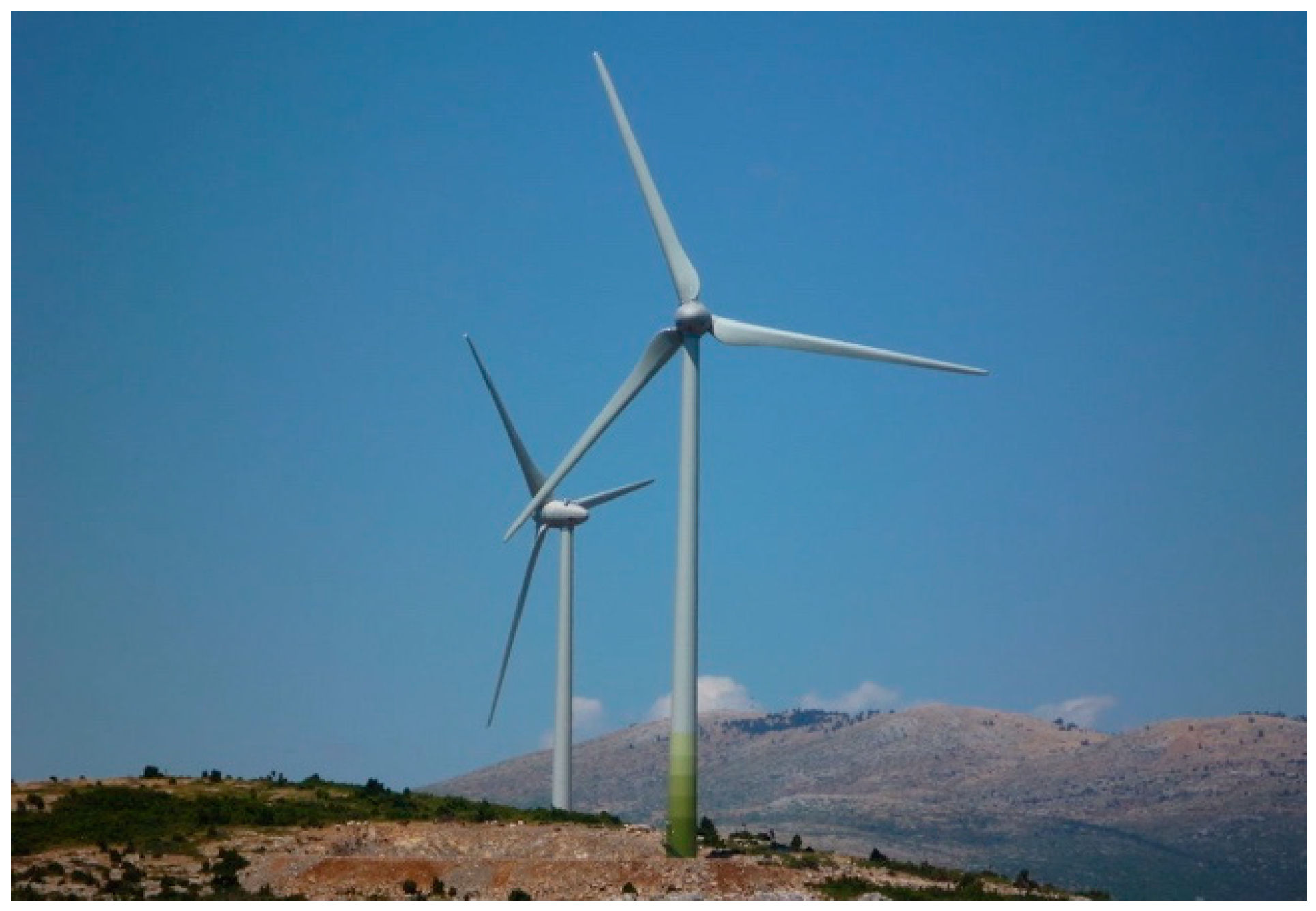
Figure 2.
Reference power curve (data from [30]) and data for turbine #1.
Figure 2.
Reference power curve (data from [30]) and data for turbine #1.
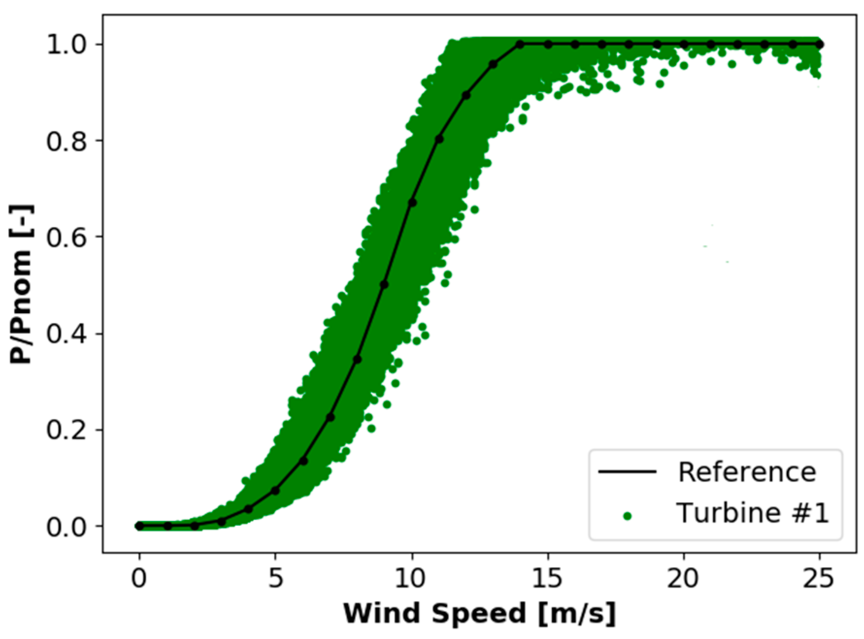
Figure 3.
Temporal downscaling of the wind power data: (a) power profile modification (10 min vs. 1 min); (b) Random values extraction for a bin of 10 min.
Figure 3.
Temporal downscaling of the wind power data: (a) power profile modification (10 min vs. 1 min); (b) Random values extraction for a bin of 10 min.
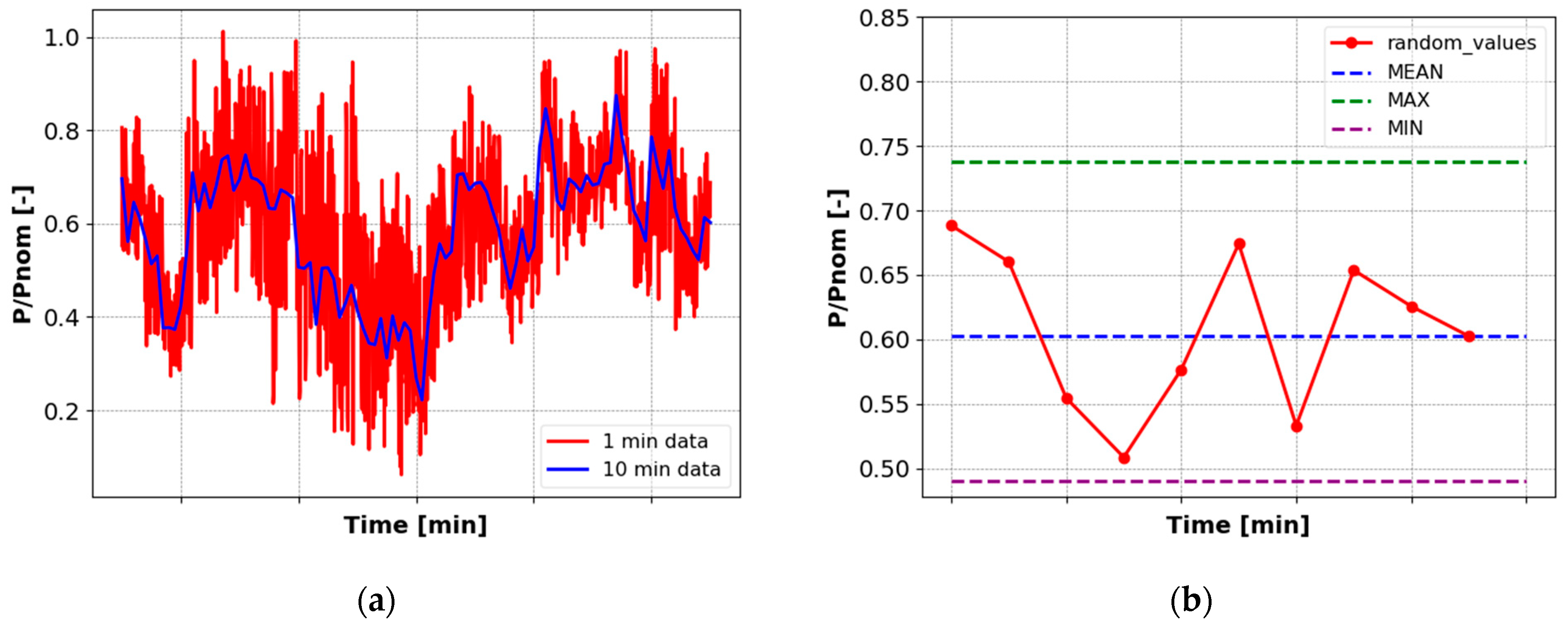
Figure 4.
Probability Density Functions (PDF) of the ramp rates 1-min data: (a) wind turbine (WT) #1 (b) WT #2.
Figure 4.
Probability Density Functions (PDF) of the ramp rates 1-min data: (a) wind turbine (WT) #1 (b) WT #2.
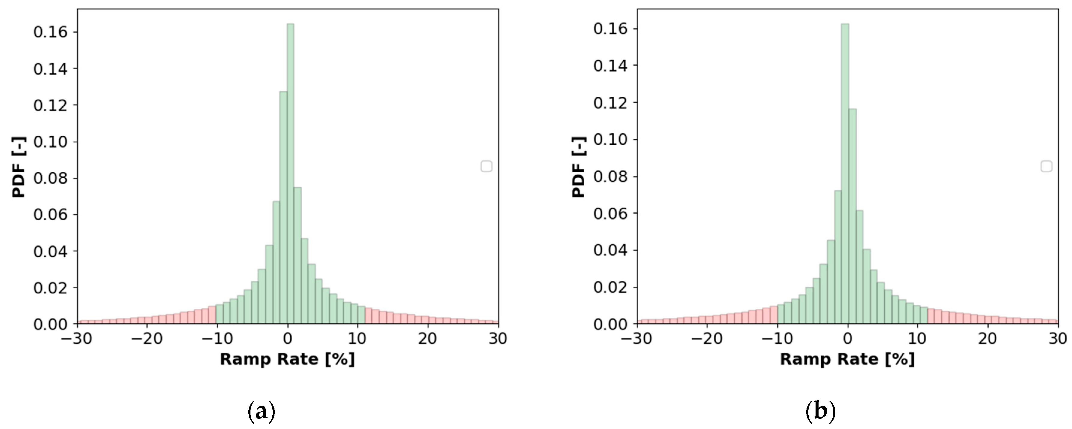
Figure 5.
Cumulative Density Functions (CDF) of the 1-min data for WT #1 and #2.
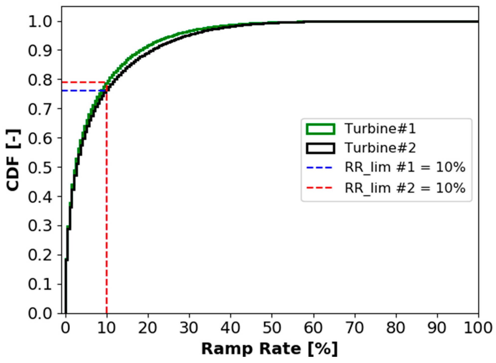
Figure 6.
Discrete Wavelet transform (DWT) application: (a) Schematic dyadic tree (b) Approximation and Detail coefficients for a sample dataset.
Figure 6.
Discrete Wavelet transform (DWT) application: (a) Schematic dyadic tree (b) Approximation and Detail coefficients for a sample dataset.

Figure 7.
Signal reconstruction for a sample dataset with the wavelet method.
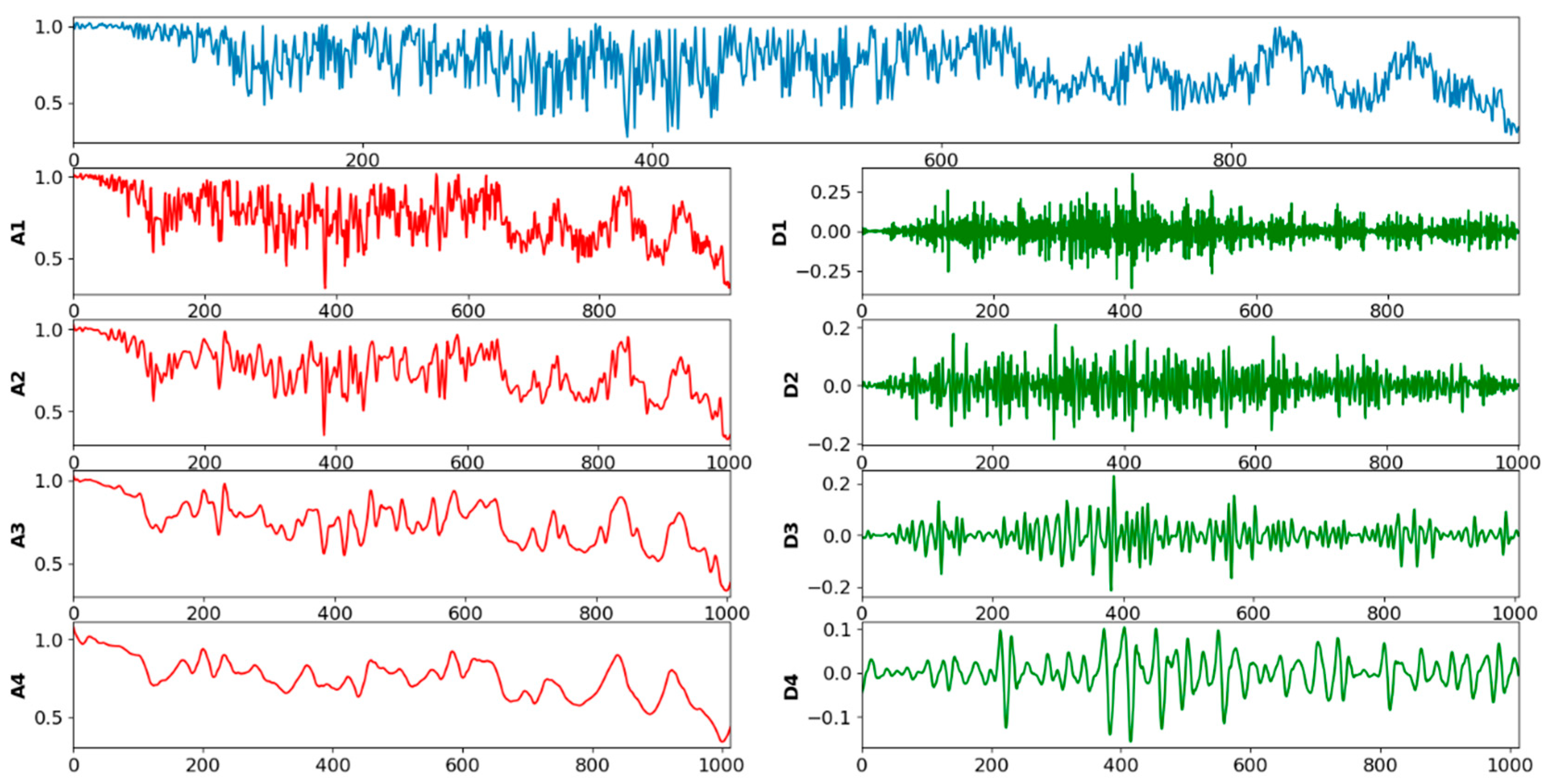
Figure 8.
Schematic flowchart of the developed power smoothing algorithm.
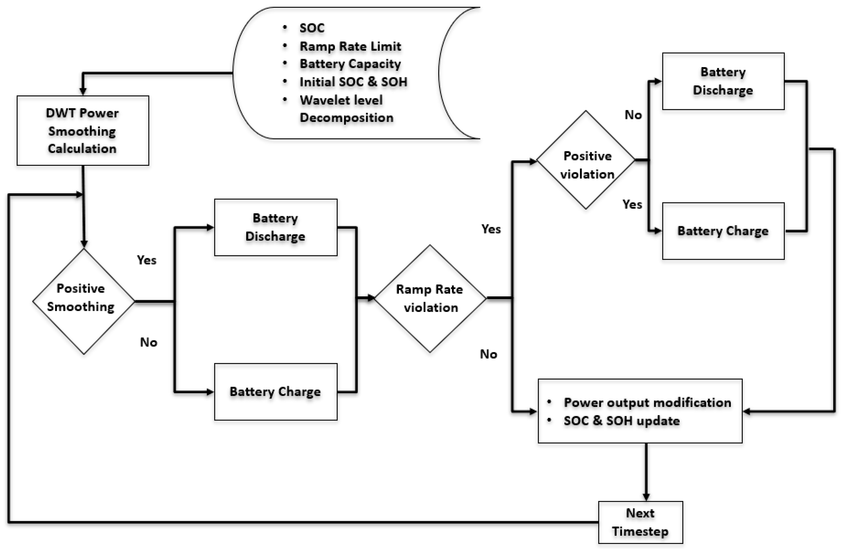
Figure 9.
Correlation between power smoothing and battery operation mode for a demonstrative time frame.
Figure 9.
Correlation between power smoothing and battery operation mode for a demonstrative time frame.

Figure 10.
Charge/Discharge efficiency vs. SOC considered for the battery (data from [49]).
Figure 10.
Charge/Discharge efficiency vs. SOC considered for the battery (data from [49]).
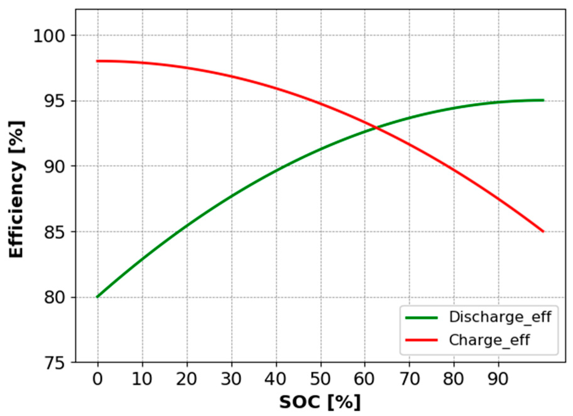
Figure 11.
Example of turbine power output modified by battery constraints.
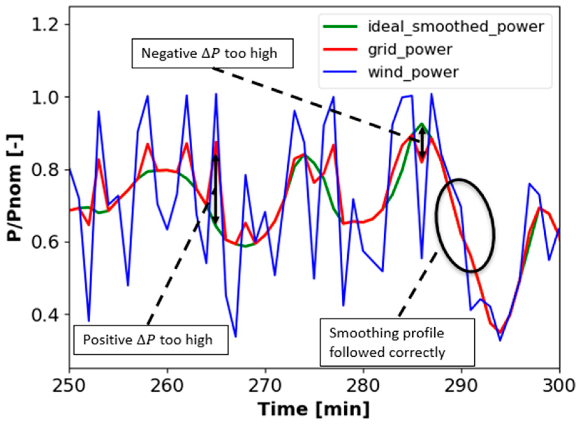
Figure 12.
Wavelet power smoothing profiles as a function of decomposition level.
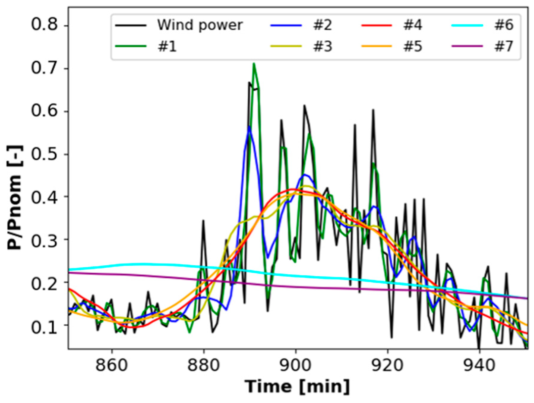
Figure 13.
Abatement Ratio vs. Battery Capacity: comparison for different wavelet levels.

Figure 14.
Abatement ratio 90% vs. 0%: (a) PDF (b) CDF.
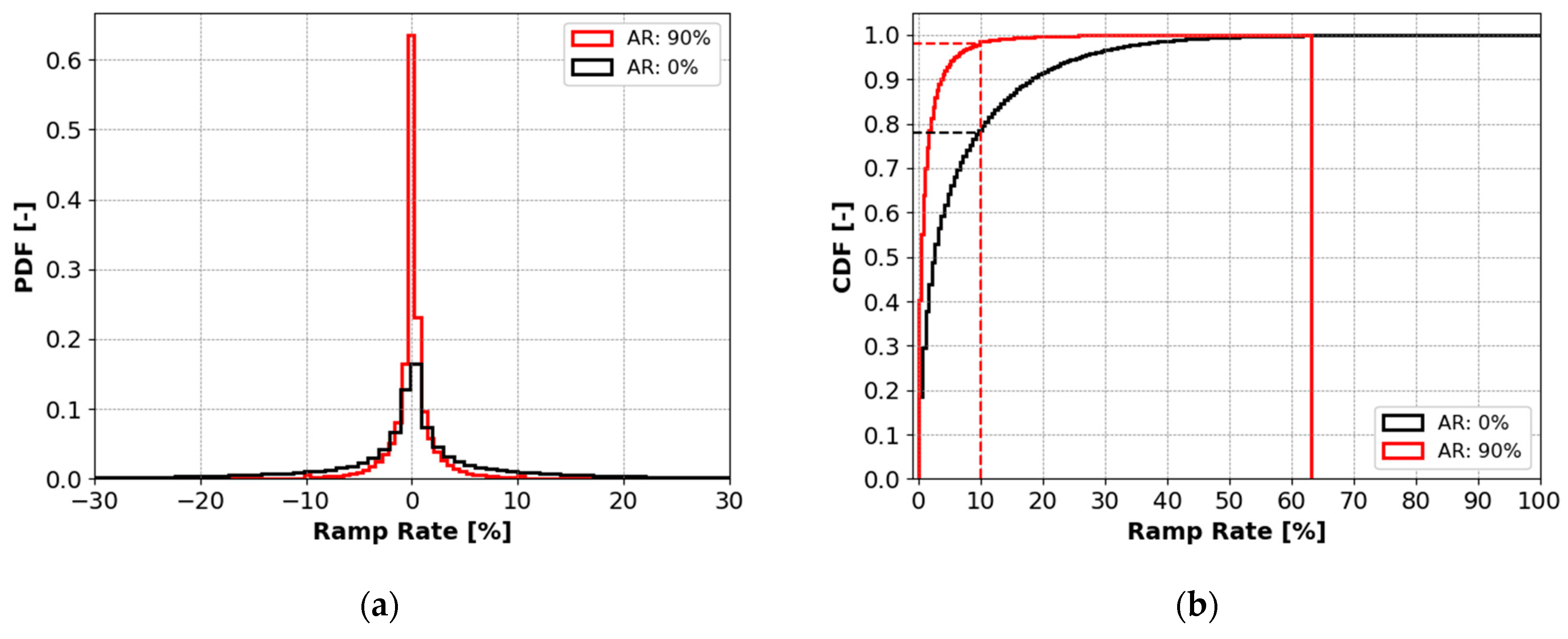
Figure 15.
Abatement Ratio vs. Battery Capacity for the considered power smoothing algorithms.
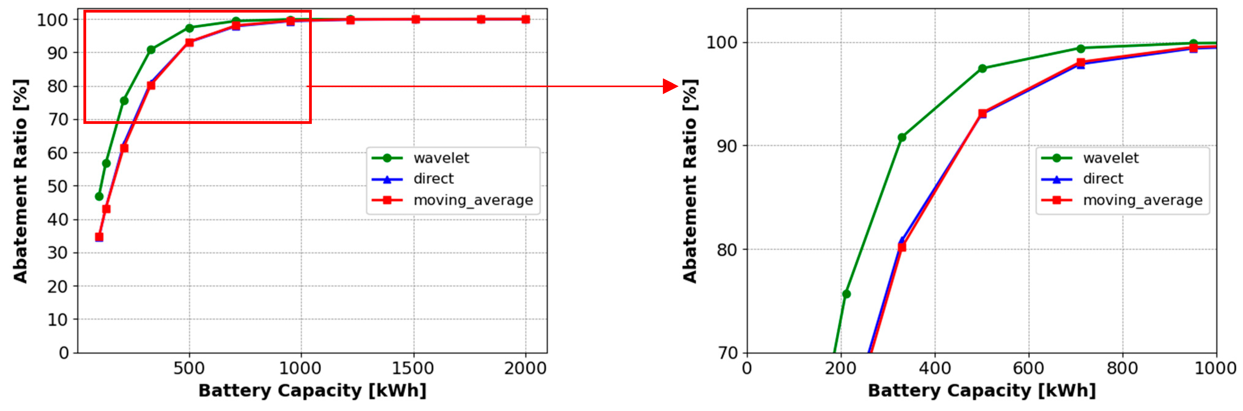
Figure 16.
Detailed comparison between the different smoothing techniques: (a) theoretical power smoothing (b) power output to the grid considering a battery capacity of 330 kWh.
Figure 16.
Detailed comparison between the different smoothing techniques: (a) theoretical power smoothing (b) power output to the grid considering a battery capacity of 330 kWh.

Figure 17.
Example of power fed into the battery (330 kWh capacity) with the different methods considered in case the battery energy storage system (BESS) operational constraints are accounted for.
Figure 17.
Example of power fed into the battery (330 kWh capacity) with the different methods considered in case the battery energy storage system (BESS) operational constraints are accounted for.
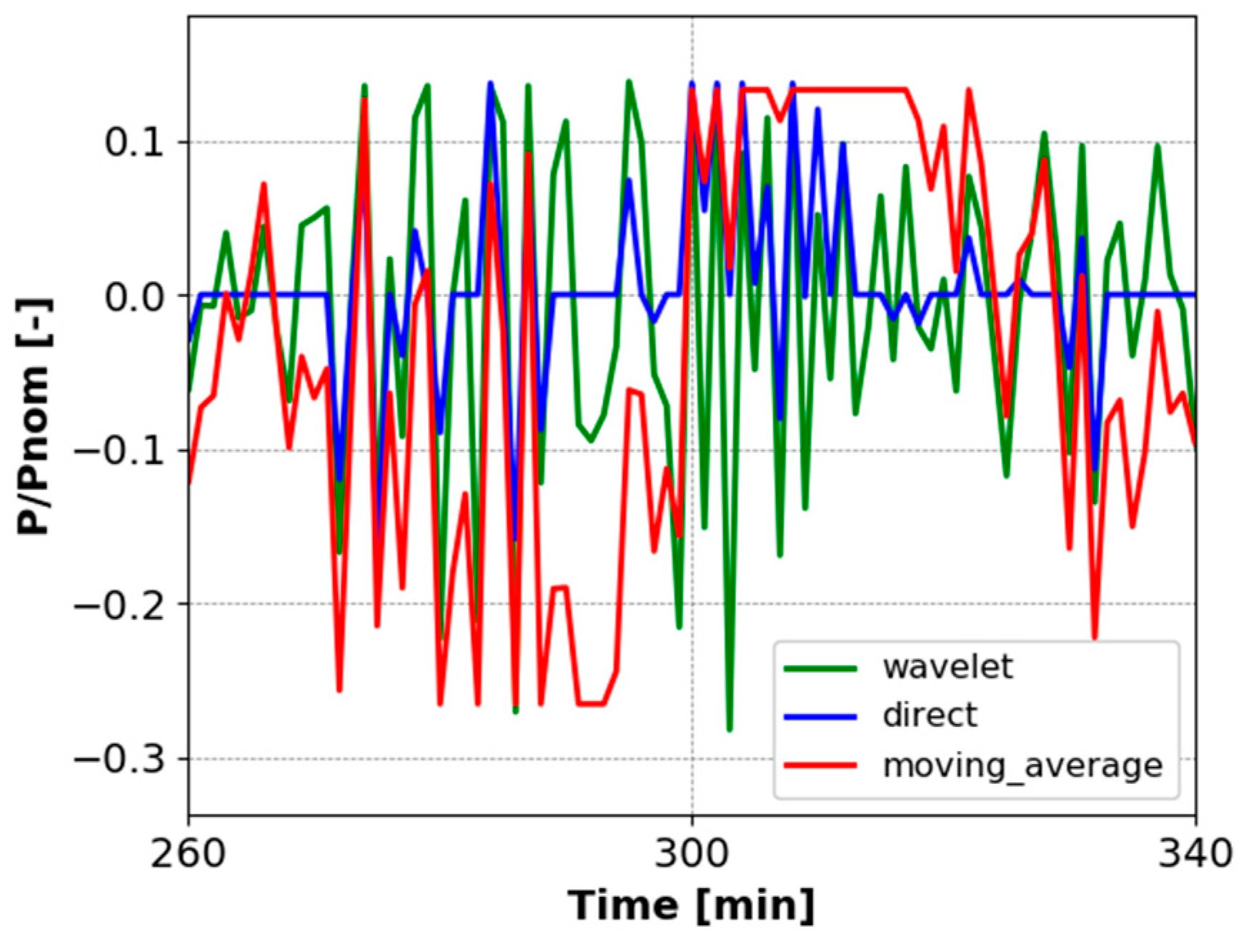
Figure 18.
Comparative analysis of SOC profiles for the three methods (same battery capacity = 330 kWh).
Figure 18.
Comparative analysis of SOC profiles for the three methods (same battery capacity = 330 kWh).

Figure 19.
Comparative analysis of SOC profiles for the three methods (Same abatement ratio (AR) = 90%), wavelet capacity 330 kWh, direct capacity 460 kWh, moving average capacity 465 kWh.
Figure 19.
Comparative analysis of SOC profiles for the three methods (Same abatement ratio (AR) = 90%), wavelet capacity 330 kWh, direct capacity 460 kWh, moving average capacity 465 kWh.
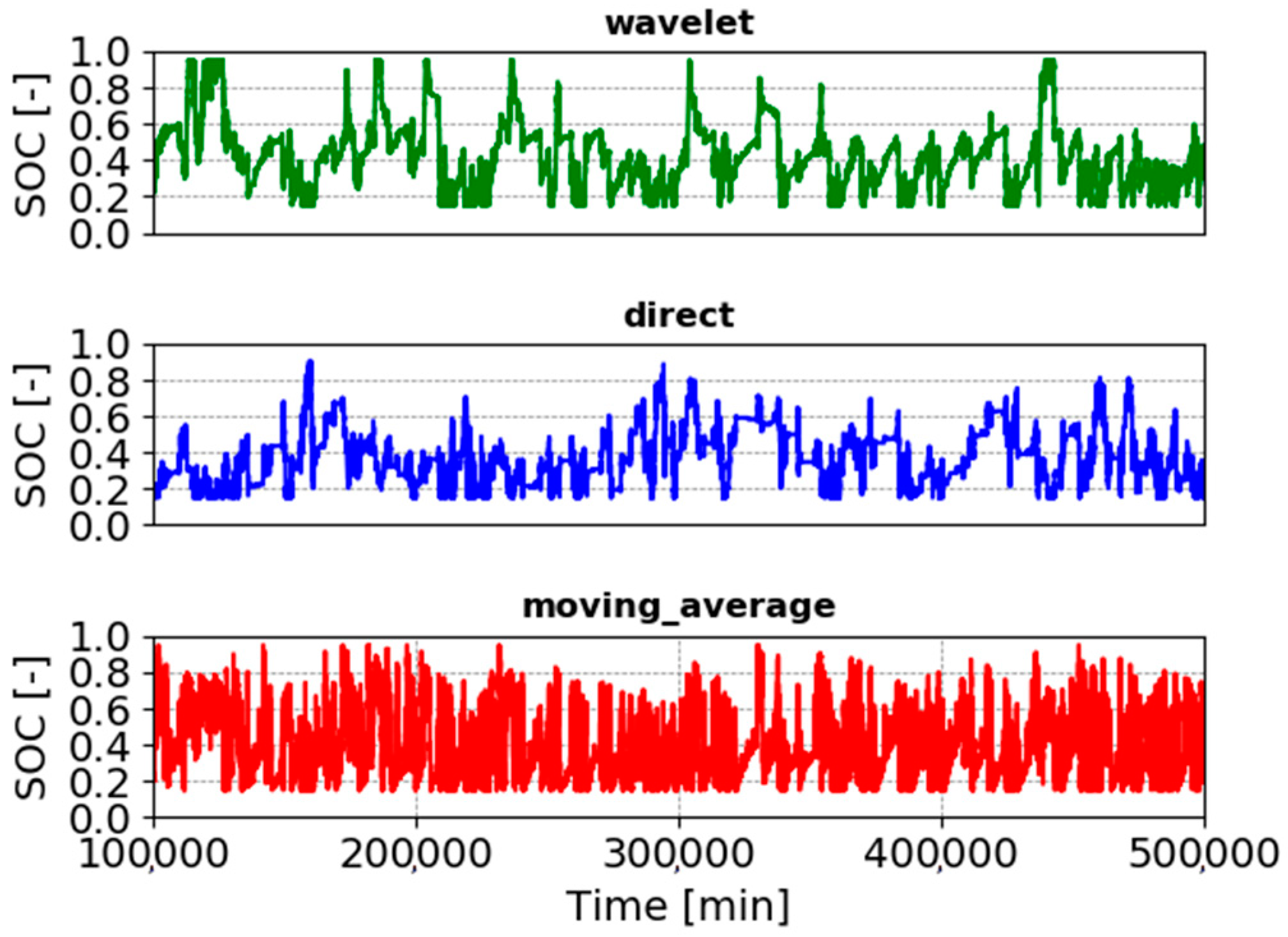
Figure 20.
Abatement Ratio vs. Battery Capacity: (a) wavelet power smoothing vs. conventional approaches (b) AR achieved with the wavelet power smoothing method using separate vs. combined ESSs.
Figure 20.
Abatement Ratio vs. Battery Capacity: (a) wavelet power smoothing vs. conventional approaches (b) AR achieved with the wavelet power smoothing method using separate vs. combined ESSs.

Figure 21.
Cost vs. Abatement Ratio for the different methods.

Figure 22.
SOH profiles (a) capacity = 330 kWh (b) AR = 90%.
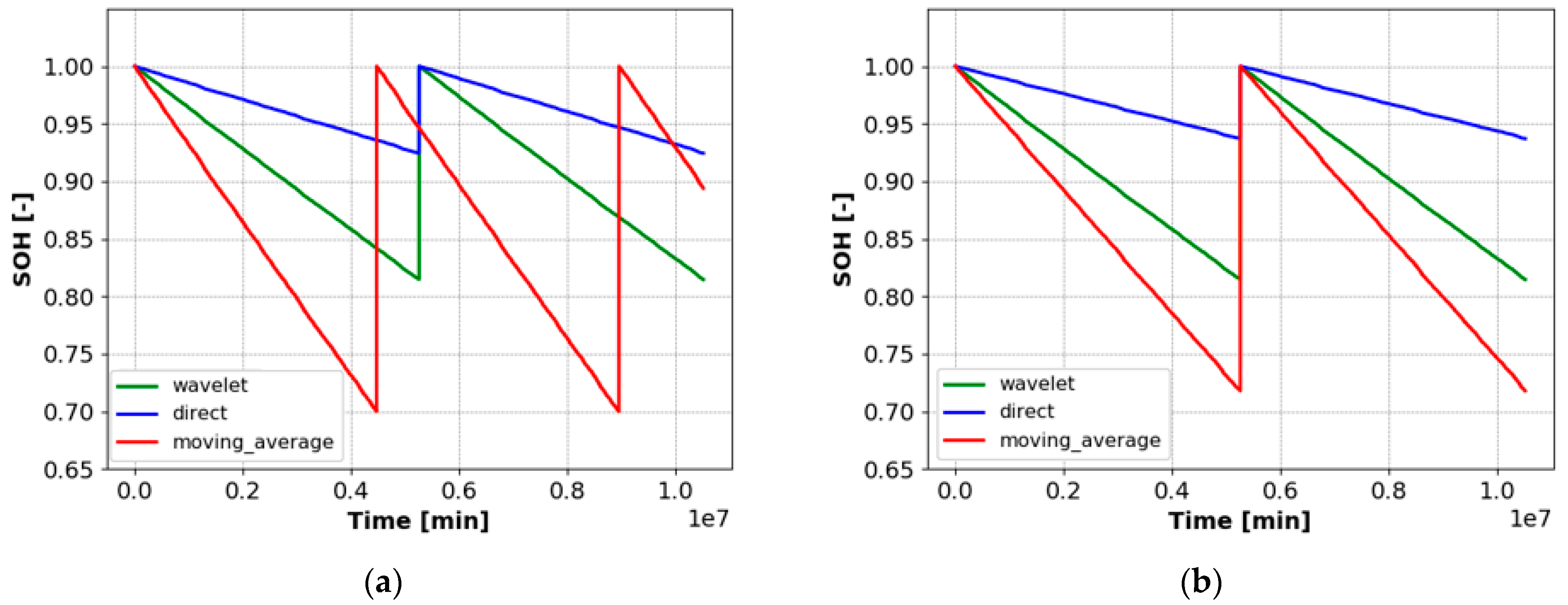
Figure 23.
Upper chart: comparison of AR capabilities and specific cost of the different methods considered. Lower chart: battery replacement times.
Figure 23.
Upper chart: comparison of AR capabilities and specific cost of the different methods considered. Lower chart: battery replacement times.
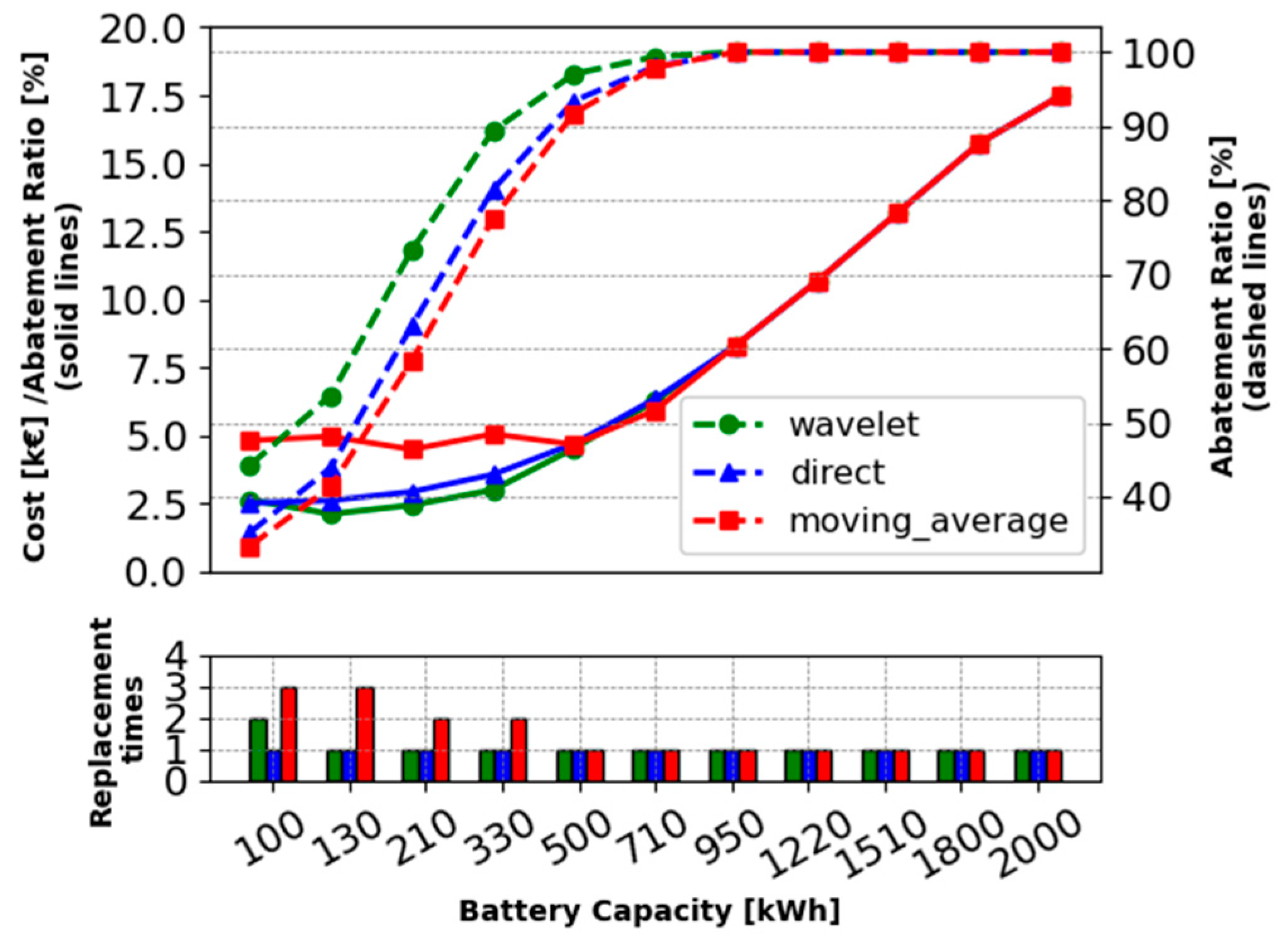
Figure 24.
Ramp rate (RR) target 5%: (a) AR vs. Battery Capacity (b) RR target comparison: 5% vs. 10%.
Figure 24.
Ramp rate (RR) target 5%: (a) AR vs. Battery Capacity (b) RR target comparison: 5% vs. 10%.

Figure 25.
Real-time control un comparison with the other methods: (a) AR vs. Battery Capacity (b) SOC profile.
Figure 25.
Real-time control un comparison with the other methods: (a) AR vs. Battery Capacity (b) SOC profile.
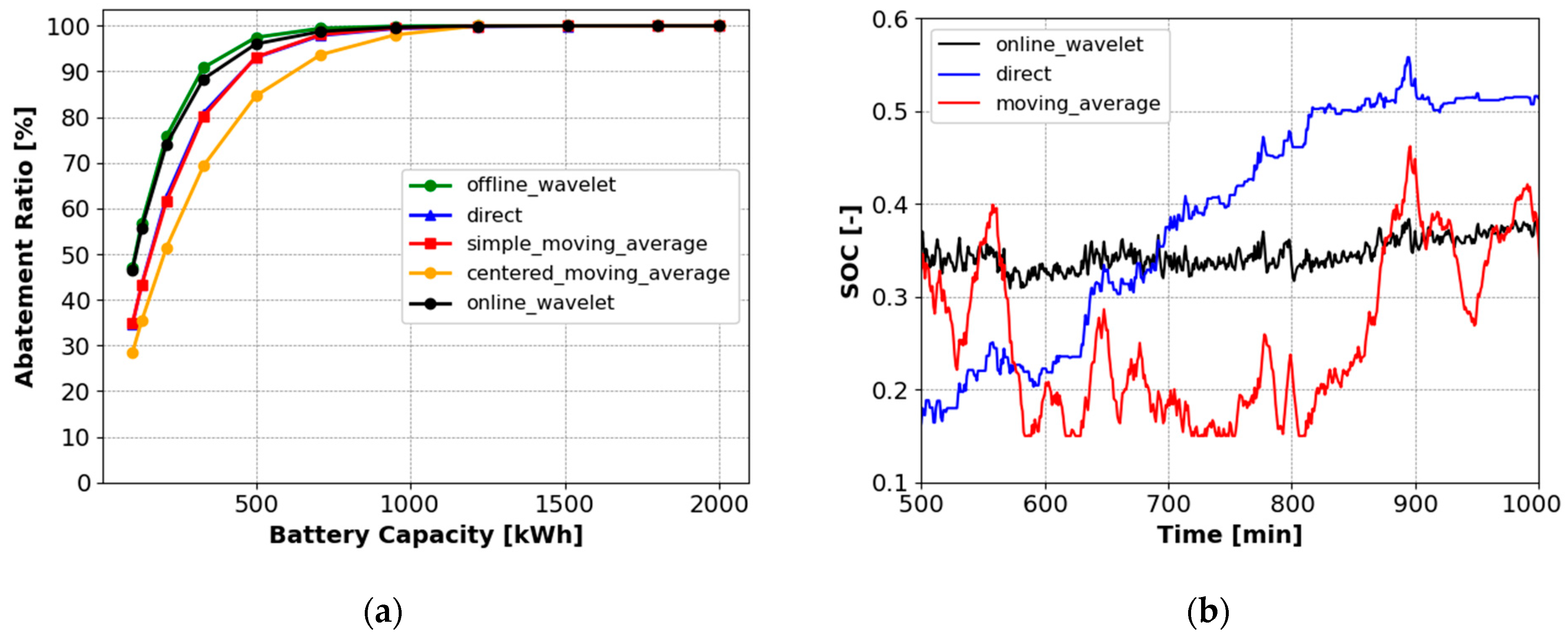
Figure 26.
Online vs. Offline: (a) Power fed into the grid (b) SOC profile.
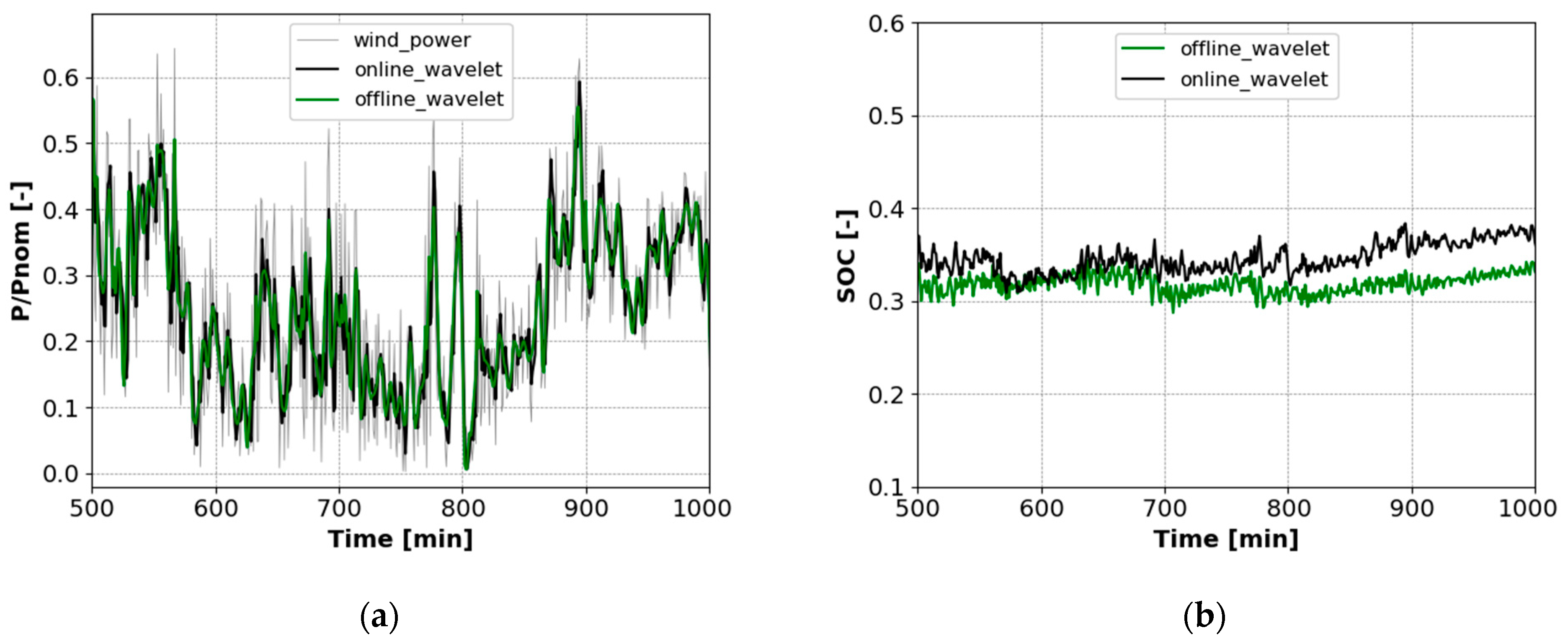

Table 1.
Ramp rate limits for some relevant countries in the world.
| Grid | Ramp Rate Limit (dP/dt) | Ref. |
|---|---|---|
| Germany | 10% Pnom per min | [15] |
| Norway | 10% Pnom per min | [26] |
| UK | No limit for wind farms up to 300 MW capacity, 50 MW/min for 300 < Pnom < 1000 40 MW/min for Pnom > 1000 MW | [15] |
| Denmark | 100 kW/s | [27] |
| Ireland | 8% Pnom per min & 4% Pnom per 10 min | [28] |
| USA | 10% Pnom per min | [19] |
| Puerto Rico | 10% Pnom per min | [4] |
| Canada | 10% Pnom per min | [19] |
| China | 3 MW/min for wind farms up to 30 MW capacity, 10% Pnom per min for 30 < Pnom < 150 MW 15 MW/min for Pnom >150 MW in size. | [19] |
Table 2.
Smoothing algorithm inputs.
| DWT features: |
|
| Ramp rate constraint: |
|
| Technical storage parameters: |
|
Table 3.
Technical specifications of the reference battery for the study.
| PHEV-1/Samsung SDI 94 Ah | |
|---|---|
| Weight | 670 kg |
| Size | 800 × 850 × 2034 mm (W × L × H) |
| Energy | 62.3 kWh |
| Nominal voltage | 662 V |
| Min. voltage | 486 V |
| Max. voltage | 747 V |
| Nominal capacity @25 °C | 94 Ah |
| Max continuous discharge current @25 °C | 230 A |
| Max continuous charge current @25 °C | 100 A |
| Cell temperature operating | 0 to 55 °C |
| Cycle lifetime EOL80%/EOL70% | 3200/5200 Cycles |
Table 4.
Algorithm correction to account for battery constraints.
| Charging Mode () |
|
| Discharging mode () |
|
Table 5.
Economic parameters.
| Battery unit cost | 500 €/kWh |
| Wind Turbine lifetime | 20 years |
| Li-ion battery lifetime | 10 years |
| Discount rate (d) | 5% |
| Inflation rate (i) | 2% |
Table 6.
SOC parameters: capacity = 330 kWh.
| Method | Average | Standard Deviation |
|---|---|---|
| Wavelet | 0.43 | 0.18 |
| Direct | 0.29 | 0.11 |
| Moving average | 0.37 | 0.19 |
Table 7.
SOC parameters: AR = 90%.
| Method | Average | Standard Deviation |
|---|---|---|
| Wavelet | 0.43 | 0.18 |
| Direct | 0.38 | 0.16 |
| Moving average | 0.40 | 0.20 |
Table 8.
Comparison between separate vs. combined configuration (AR = 90%). Wavelet-based battery management.
Table 8.
Comparison between separate vs. combined configuration (AR = 90%). Wavelet-based battery management.
| Layout | BESS Capacity [kWh] |
|---|---|
| Separate systems | 690 |
| Combined system | 445 |
| Increment | −35% |
Table 9.
Discounted lifetime cost comparison between the three methods (AR = 90%).
| Method | BESS Capacity [kWh] | Discounted Cost [k€] |
|---|---|---|
| Wavelet | 330 (-) | 288 (-) |
| Direct | 460 (+39%) | 402 (+39%) |
| Moving average | 465 (+41%) | 406 (+41%) |
Table 10.
AR results for different lw and ls combinations. AR is calculated on entire dataset used throughout Section 5.
Table 10.
AR results for different lw and ls combinations. AR is calculated on entire dataset used throughout Section 5.
| Moving Window Length (lw) | ||||||
|---|---|---|---|---|---|---|
| 4 | 8 | 16 | 24 | 32 | ||
| Symmetric Extension Length (ls) | 4 | 85.49217 | 87.9971 | 88.2814 | 88.2782 | 88.2782 |
| 8 | / | 88.0969 | 88.3445 | 88.3482 | 88.3303 | |
| 16 | / | / | 88.3448 | 88.3446 | 88.3447 | |
| 24 | / | / | / | 88.3439 | 88.3439 | |
| 32 | / | / | / | / | 88.3439 | |
Publisher’s Note: MDPI stays neutral with regard to jurisdictional claims in published maps and institutional affiliations. |
© 2021 by the authors. Licensee MDPI, Basel, Switzerland. This article is an open access article distributed under the terms and conditions of the Creative Commons Attribution (CC BY) license (https://creativecommons.org/licenses/by/4.0/).
Share and Cite
MDPI and ACS Style
Mannelli, A.; Papi, F.; Pechlivanoglou, G.; Ferrara, G.; Bianchini, A. Discrete Wavelet Transform for the Real-Time Smoothing of Wind Turbine Power Using Li-Ion Batteries. Energies 2021, 14, 2184. https://doi.org/10.3390/en14082184
AMA Style
Mannelli A, Papi F, Pechlivanoglou G, Ferrara G, Bianchini A. Discrete Wavelet Transform for the Real-Time Smoothing of Wind Turbine Power Using Li-Ion Batteries. Energies. 2021; 14(8):2184. https://doi.org/10.3390/en14082184
Chicago/Turabian StyleMannelli, Andrea, Francesco Papi, George Pechlivanoglou, Giovanni Ferrara, and Alessandro Bianchini. 2021. "Discrete Wavelet Transform for the Real-Time Smoothing of Wind Turbine Power Using Li-Ion Batteries" Energies 14, no. 8: 2184. https://doi.org/10.3390/en14082184
Note that from the first issue of 2016, this journal uses article numbers instead of page numbers. See further details here.