
Using EMPHASIS for the Thermography-Based Fault Detection in Photovoltaic Plants
by
 , , ,
, , ,
Antonio Pio Catalano
* ,
,
Ciro Scognamillo
 ,
,
Pierluigi Guerriero
,
Santolo Daliento
and
Vincenzo d’Alessandro
Department of Electrical Engineering and Information Technology, University ‘Federico II’, 80125 Naples, Italy
*
Author to whom correspondence should be addressed.
Energies 2021, 14(6), 1559; https://doi.org/10.3390/en14061559
Submission received: 16 November 2020
/
Revised: 4 March 2021
/
Accepted: 5 March 2021
/
Published: 11 March 2021
(This article belongs to the Topic Electrothermal Modeling of Solar Cells and Modules)
Abstract
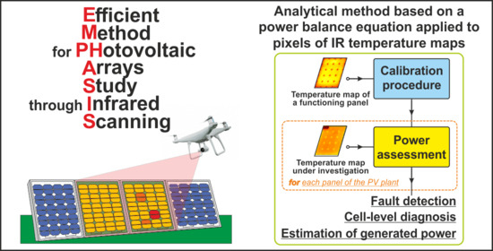
:In this paper, an Efficient Method for PHotovoltaic Arrays Study through Infrared Scanning (EMPHASIS) is presented; it is a fast, simple, and trustworthy cell-level diagnosis method for commercial photovoltaic (PV) panels. EMPHASIS processes temperature maps experimentally obtained through IR cameras and is based on a power balance equation. Along with the identification of malfunction events, EMPHASIS offers an innovative feature, i.e., it estimates the electrical powers generated (or dissipated) by the individual cells. A procedure to evaluate the accuracy of the EMPHASIS predictions is proposed, which relies on detailed three-dimensional (3-D) numerical simulations to emulate realistic temperature maps of PV panels under any working condition. Malfunctioning panels were replicated in the numerical environment and the corresponding temperature maps were fed to EMPHASIS. Excellent results were achieved in both the cell- and panel-level power predictions. More specifically, the estimation of the power production of a PV panel with a shunted cell demonstrated an error lower than 1%. In cases of strong nonuniformities as a PV panel in hotspot, an estimation error in the range of 9–16% was quantified.
1. Introduction
In the last decades, both the growing efficiency and the cost reduction in photovoltaic (PV) plants have contributed to their wide diffusion in customer applications [1]. Currently, emerging countries face the rising energy demand of their economy by installing large PV plants, which are steadily moving from ancillary to main energy sources [2,3,4]. On the other hand, in developed countries, the PV market is enhanced by the diffusion of innovative smart grids and of private electric mobility [5], both supported by the availability of battery energy storage systems [6,7].
However, grid parity can only be reached by providing the full functionality of energy plants and by reducing maintenance costs [8,9]. According to smart operation and maintenance approaches, effective monitoring systems are needed to timely detect any malfunction event and yield loss [10], thus (i) reducing production issues and (ii) allowing an accurate evaluation of failures.
PV plants are plagued by numerous types of faults [11]. The faults on the AC side are mainly caused by inverter failures and/or undesired activation of interface mechanisms [12,13,14]. On the DC side, where the plant appears as a complex structure, an individual PV panel can be typically affected by delamination, browning, cracks, snail trails, ribbons soldering issues, bypass diodes failures, and electric arcs [15]. At a cell-level, shunted cells and localized hotspots may be induced by aging, partial shadow, and overheating [16,17,18].
For the aforementioned reasons, diagnosis represents a valuable strategy to detect and analyze the reduction in PV plant reliability [19]. The literature is populated by many fault-detection approaches [20,21,22,23,24,25,26,27,28,29,30,31,32,33,34,35,36,37,38,39], a first classification of which can be based on their granularity. While in [23] the investigation involves the whole PV plant, methods aimed at monitoring PV strings are shown in [24,25]. The granularity is even higher in the approach presented in [26,27], in which sensing circuits to be mounted on each PV panel are exploited. It is clear that an increased granularity comes with a more precise diagnosis power; on the other hand, it implies higher costs as well as complex procedures.
As stated in [28,29,30,31,32], the trade-off between granularity and cost can be overcome by exploiting diagnosis approaches based on thermography. More specifically, the use of drones to capture infrared (IR) images of the panel was found to be a convenient solution to mitigate the maintenance costs [33,34,35,36]. In [31,32], the IR images are fed to heuristics methods, whereas neural networks are adopted in [37,38,39]. However, these strategies (i) rely on time-demanding preliminary stages (e.g., the training of neural networks), (ii) require the use of additional sensors, and (iii) may partially interrupt the power production of the plant. It must also be remarked that these approaches are only devoted to identifying the type of fault and they are not able to recognize the actual working conditions of the panel.
In [40], an analytical diagnosis method based on aerial IR scanning was introduced. Besides being able to detect and classify the fault, it allows the identification of the electrical power generated (or even dissipated) by the individual cells composing PV panels. To carry out a cell-level power assessment, the method in [40] was based on a power balance law applied to on-field temperature maps of PV panels under their actual working conditions; this was possible since the approach does not demand the stop of the PV plant power production. A new version of the same method requiring a reduced number of sensors was presented in [41]. Although both approaches allowed identifying localized faults, their cell-level electrical power estimations were still fairly imprecise.
This paper presents three variants of Efficient Method for PHotovoltaic Arrays Study through Infrared Scanning (EMPHASIS), which is an upgraded version of the methods shown in [40,41]. If compared with its previous versions, EMPHASIS benefits from the accuracy in the cell-level power assessment. These improvements were obtained by adopting (i) a pixel-level power balance equation increasing the granularity and (ii) temperature-dependent parameters accounting for the nonlinear (NL) thermal effects. The evaluation of the accuracy of the cell-level power prediction was performed through a strategy based on “simulated experiments.” Instead of experimental temperature maps, EMPHASIS was used to examine numerical, yet realistic, ones corresponding to a known power pattern. Then, the predicted values were compared with the already known ones. A procedure was devised in order to extract the abovementioned numerical temperature maps of functioning and malfunctioning commercial PV panels. This procedure was appropriately tuned by on-field measurements and combines an electrothermal (ET) macrocircuit in a SPICE-like environment and three-dimensional (3-D) purely-thermal simulations in a finite-element method (FEM) software package. It is worth noting that such a procedure is not to be conducted by the EMPHASIS end users, since it was only adopted in the “simulated experiments.”
2. EMPHASIS
EMPHASIS is an innovative method aimed to predict the effective working conditions of any PV panel (even malfunctioning ones) by means of the mere knowledge of the temperature field on the front surface (Tglass). To obtain the predictions, the whole top surface of the panel has to be partitioned into a specific set of disjoint areas A, to which the following power balance equation is applied:
where G and Tamb correspond to solar irradiance and ambient temperature, respectively.
The single variables in Equation (1) can be classified as: input physical quantities (G, A, Tamb), tuning parameters (rA), quantities to be evaluated (Tavg,A and Pout,A), and generated electrical powers (Pg,A). On the left side of Equation (1), 0.95⸱G⸱A corresponds to the solar power impinging on the area A and takes into account a loss of 5% due to reflection mechanisms; such an input term has to be balanced by the sum of the 3 contributions described in the following:
- Pg,A is the electrical power generated (or, if negative, dissipated) in the area A; the quantity 0.95⸱G⸱A–Pg,A corresponds to the power giving rise to the thermalization process.
- The ratio between the temperature increment averaged on A (Tavg,A–Tamb) and the positive quantity rA is representative of the upward heat flux through the panel front surface (i.e., the thermal power vertically flowing from the cells to the ambient). Here, rA has the dimensions of a thermal resistance [K/W] and accounts for the thermal behavior of the panel. It depends on the panel characteristics (i.e., geometry and materials) as well as on the ambient conditions. Since the PV panel temperature is typically higher than the ambient one, such a ratio is expected to be positive.
- The thermal power Pout,A represents that the heat horizontally moving in and out from the specific area A; Pout,A is positive (negative) in presence of an outgoing (ingoing) effective horizontal heat flux.
The power balance solely neglects the downward heat flux; however, this contribution only marginally influences the power balance accuracy. The bottom surface is usually not prone to the heat disposal because of (i) its poor convective-radiative effects and (ii) the low thermally conductive materials (e.g., the Tedlar) positioned on the back.
The quantities to be evaluated Tavg,A and Pout,A are obtained by elaborating the temperature maps; while Tavg,A corresponds to the Tglass averaged on the area A, Pout,A is evaluated according to the following equation:
where ∇T is the two-dimensional (2-D) temperature gradient, EA represents the border of the area A, is the unit normal vector pointing out from EA, while tglass and kglass are the glass thickness and thermal conductivity, respectively. In Equation (2), the heat is assumed to flow only through the front glass, since the contribution involving the thin layer encapsulating the cells is typically negligible.
EMPHASIS can be subdivided into two analytical stages that require (i) the electrical and thermal features of the panel under investigation and (ii) the knowledge of G and Tamb. Both stages exploit the power balance equation with different targets:
- the first stage, also referred to as calibration procedure, is performed only once on temperature maps of functioning panels, the generated power of which (Pg,panel) must be known. The calibration procedure identifies the rA distribution—representing the only unknown in Equation (1). While Pout,A and Tavg,A are obtained as stated before, each Pg,A value can be derived as Pg,panel∙A/Aglass, where Aglass is the area of the panel front surface;
- the second stage, denoted as power assessment, is performed on temperature maps of panels working under unknown electrical conditions (i.e., Pg,panel is undetermined). To identify the energy production of the panel, the power assessment (i) exploits the rA distribution extracted in the calibration procedure and (ii) solves Equation (1) for Pg,A.
It must be remarked that the temperature maps of all the panels—including the ones needed in the calibration procedure—are to be taken in a relatively short amount of time to ensure the same ambient conditions. It is noteworthy to highlight that rA can be either temperature-independent (Section 2.1 and Section 2.3) or temperature-dependent (Section 2.2), as a result of the calibration procedure.
The accuracy of the method strongly depends on the partitioning of the front panel surface. In [40,41], A coincided with the cell area (Acell); this choice neglects the temperature gradients internal to the PV cells that may reduce the accuracy of the method. EMPHASIS solves this issue by applying Equation (1) to the individual pixels of the temperature maps, thus reaching the maximum granularity level. By considering A = Apixel, Equation (1) becomes:
where i is the index of the individual pixel and Pg,i, Ti, ri, and Pout,i correspond to pixel-level quantities. In this hypothesis, during the power assessment stage, the evaluated output is represented by the Pg,i distribution; to obtain the cell-level electrical powers (Pg,cells), Pg,i is then integrated over the corresponding cell area. A schematic representation of the EMPHASIS workflow is shown in Figure 1. It must be underlined that EMPHASIS is developed to be applied to real PV panels; the calibration procedure is performed on a functioning panel (with no significant mismatches between cells). Then, the ri distribution serves to investigate temperature maps and to assess the corresponding Pg,i values.
The following subsections outline three pixel-level EMPHASIS variants; they differ in both the calibration procedure and the power assessment stages.
2.1. Standard Approach
The calibration procedure of the standard approach requires one temperature map taken under known working conditions. In the calibration stage, the ri distribution is evaluated according to
Equation (4) generalizes the power balance useful for the calibration procedure, which can be performed on PV panels operating under any working condition, that is, regardless of the Pg,i distribution. On the other hand, a temperature map typically adopted is obtained under open-circuit (OC) conditions; it turns out to be a convenient choice because of the Pg,i values—all of them trivially being 0 W. Then, the analysis moves towards the temperature maps of the actual panels to be investigated, the electrical working conditions of which are unknown. The power assessment is carried out by solving
where the ri values correspond to the ones obtained in the previous calibration procedure.
2.2. NL-Corrected Approach
The NL-corrected approach aims to mitigate the errors introduced by the NL effects described in Section 3.3. Its calibration procedure requires two temperature maps and the corresponding Pg,panel values. A typical choice is represented by panels working under OC and maximum-power-point (MPP) conditions. The two ri distributions are evaluated according to Equation (4); then, a set of linear ri(T) functions is obtained by a (2-point) interpolation.
Once the calibration procedure is carried out, the power assessment is conducted on the panels to be examined by solving
2.3. Differential Approach
Two temperature maps (e.g., under OC and MPP conditions) can also be exploited in the differential approach described in the following. For each temperature map (namely, map #1 and #2), Equation (3) can be applied.
By subtracting Equation (8) from Equation (7) and assuming r1,i = r2,i = rd,i, it follows:
For the sake of clarity, it must be remarked that the two r1,i and r2,i distributions do not coincide because of the NL nature of the thermal problem. However, a preliminary study demonstrated that this assumption is reasonable: several NL FEM simulations have been performed and the discrepancy between the two distributions was ~0.7% on average.
After the rd,i extraction, one of the two temperature maps exploited in the calibration procedure has to be also accounted for in the power assessment stage; for instance, by considering map #1, the power assessment can be computed according to
As Equation (10) clearly states, the differential approach solves the issue related to the lack of some parameters. More specifically, it can be applied without the knowledge of the G and Tamb values; it therefore allows avoiding ad hoc sensors that introduce inevitable measurement errors. On the other hand, the constraint of a short time between the shoots of the temperature maps adopted in the calibration procedure is even stricter; Equation (9) is indeed more valid as such a time decrease.
3. “Simulated Experiments” Methodology
The study presented in this section was conceived with the ambition of validating EMPHASIS, and it is therefore not to be adopted by the end users. It aims to evaluate the method accuracy by processing temperature maps of commercial PV panels. A way to obtain such temperature maps is to exploit aerial thermography (e.g., drones equipped with IR cameras). However, the adoption of experimental maps would lead to some limitations: it is not always possible to create ad hoc malfunctioning (e.g., localized hotspots or shunted cells) and, in addition, aerial IR scanning does not provide the cell-level working conditions of the PV panel—needed in the accuracy evaluation stage. These issues were solved by adopting a strategy based on “simulated experiments,” which can be explained/described as follows:
- a commercial PV panel (Section 3.1) was tested by on-field measurements (Section 3.2);
- an ET macrocircuit in a SPICE-like environment was exploited to emulate the ET behavior of the PV panel (Section 3.3);
- a real PV panel was replicated in a commercial FEM software package (Section 3.4) and thermal simulations were performed to extract temperature maps under many working and environmental conditions. Such maps emulate the realistic PV panel thermal behavior as if they were taken through IR scanning. The key point is that—in contrast to IR scanning—the cell-level working conditions (i.e., the Pg,cell distribution obtained by the ET macrocircuit) are known and can be used as a reference; these temperature maps were fed to EMPHASIS that provided a prediction of the Pg,cell values.
The method accuracy was evaluated by comparing such a prediction with the reference Pg,cells.
3.1. PV Panel under Investigation
EMPHASIS can in principle be applied to PV panels of any shape, size, and number of cells; in this work, the “simulated experiments” focused on the commercial PV panel described in [42]. The panel is based on monocrystalline silicon (Si) and comprises 40 series-connected cells arranged in 10 rows and 4 columns according to Figure 2, which also highlights the left and right subpanels. The individual cell is hexagonal in shape and Acell was estimated to be 72.8 cm2. The electrical rates reported in the datasheet are referred to the standard test conditions (STC), that is, standard solar irradiance (GSTC) of 1000 W/m2, 1.5 Air Mass, and Tamb = 25 °C. The open-circuit voltage (VOC) and the short-circuit current (ISC) under STC are 24.6 V and 2.81 A, respectively; under the same conditions, the MPP voltage (current) is 20.2 V (2.48 A) leading to a maximum Pg,panel value of ~50 W.
Figure 3 illustrates the technology of the PV panel under analysis. On the back, a thin Tedlar sheet is positioned to prevent the entrance of water and steam. The 150 μm-thick Si cells are embedded in the middle of an ethylene vinyl acetate (EVA) layer, the thickness of which is 950 μm. A 3 mm-thick glass covering the whole panel acts as both an electrical insulator and a protection for the PV cells underneath. The panel is surrounded by an aluminum frame, which provides a mechanical support to the assembly by sealing the abovementioned layers together. The width, length, and thickness of the panel are W = 55.5 cm, H = 71.9 cm, and t = 3.4 cm, respectively.
3.2. On-Field Measurements
On-field measurements were conducted on the previously described panel mounted with a tilt angle β = 30° and oriented with an azimuth angle (positive from south to west) γ = −16° on the rooftop of the Department of Electrical Engineering and Information Technology in Naples, Italy (latitude ϕ = 40.84° and longitude λ = 14.25°). The experiment was carried out on a sunny day of May in Naples at 13:00 with a measured Tamb = 22.9 °C and wind speed of ~2 m/s (detected by means of an anemometer); the panel was previously cleaned. An ammeter was connected to the power terminals of the panel and ISC,exp was measured. The experimental irradiance (Gexp) was then evaluated according to the following equation:
An irradiance value Gexp = 865 W/m2 was obtained.
As a second step, a thermal camera FLUKE TiS55 (resolution 220 × 165) [43] was exploited to acquire the temperature map of the panel under OC conditions. Figure 4 shows the map obtained through IR scanning at a distance of ~2.5 m. The original picture was subject to a post-processing stage consisting in (i) a visual inspection to delimitate the boundaries of the PV panel, (ii) a manual parallax correction, and (iii) a 2-D Gaussian filter reducing the quantization error introduced by the IR sensor.
By processing the temperature map in Figure 4, the average temperature increment of each cell (ΔTavg,cell) was computed and the self- and mutual-heating resistances (RSMHs) values were obtained according to
The RSMHs have the dimension of a thermal resistance (K/W)) and account for the self- and mutual-heating effects of the individual cells, as well as the heat exchange mechanisms of the panel. In the case study, the RSMH values span in the range of 8–10 K/W.
3.3. SPICE Electrothermal Model
The RSMHs were used to account for the power-temperature feedback in an ET macrocircuit describing the panel in a SPICE-like solver [44]. According to Figure 5, each cell was described by coupling an electrical behavioral model and its thermal feedback circuit. The electrical model is inspired by the work of Guerriero et al. [45], in which the widely known single diode equivalent circuit [46] was suitably extended by means of analog behavioral modeling blocks. The latter were exploited to include (i) the cell-level avalanche current (IAV,cell) and (ii) the temperature dependence of the main electrical model parameters, such as the mobility, the series resistance (Rs), and the photogenerated current (Iph). The power dissipated by the cell (PD) was evaluated by the difference between the impinging one (corresponding to 0.95∙G∙Acell) and the electrical power, which is given by the product of the cell output current (Icell) and voltage (Vcell).
Concerning the ET feedback, the circuit shown in Figure 5 makes use of the thermal equivalent of the Ohm’s law [47]. PD is fed as a current, while the cell temperature (Tcell) corresponds to the voltage drop on the series of the RSMH and the voltage generator Tamb, which can vary depending on the case study. Tcell, in turn, is supplied to the electrical behavioral model [48]. The 40 cells were then connected in series and two Si-based bypass diodes were included to define the left and right subpanels. The resulting macrocircuit is depicted in Figure 6.
The implemented macrocircuit offers the key feature of varying the single parameters of each cell in order to emulate:
- a variation of the environmental conditions by acting on Tamb and G;
- any malfunction event, such as a shunt fault by simply reducing the shunt resistance (Rsh) value of the individual cells;
- a partial shading that may lead to localized hotspots, emulated by reducing the G value of the shaded cells.
In addition to the abovementioned advantages, the ET macrocircuit enabled the evaluation of the EMPHASIS accuracy by providing the Pg,cell reference distributions to be used in the “simulated experiments.”
3.4. FEM Simulations
The exact replica of the PV panel under investigation was automatically built in COMSOL Multiphysics [49] by means of an in-house routine [50,51,52] addressed to thermal-only FEM simulations. Such a routine exploits the livelink between MATLAB and COMSOL Multiphysics and is briefly described in the following. The 2-D information of the PV panel is included in a graphic data system file, which is organized in layers and serves as a starting point. Then, the layout is extruded into the 3rd dimension by assigning to each layer a thickness and a quote on the z-axis (i.e., the vertical one). Given the 3-D domain, each layer is associated to the corresponding material. Table 1 summarizes the thermal conductivity values k(T0) of the materials composing the domain, where T0 + 273° (T0 = 27 °C) is the reference temperature in the FEM solver. The structure built in COMSOL is represented in Figure 7a.
The domain was subsequently discretized into a tetrahedral mesh (Figure 7b), with a number of elements and degrees of freedom of ~1.8 and ~2.3 M, respectively. In the thermal problem, the power generation was then set by attributing to the individual heat sources (coinciding with the PV cells) the corresponding PD value evaluated according to
where Pg,cell represents the reference distribution computed by the ET macrocircuit and used in the “simulated experiments.” The solution of the thermal problem was finally carried out (Figure 7c) by the NL solver embedded in the FEM software package. On average, the time for a single steady-state simulation amounted to 30 min on a PC equipped with an Intel Core i7-7700 and a 16 GB RAM.
Convective and radiative BCs were accounted for in the thermal problem. For what concerns the convection, it was activated through two heat transfer coefficients on the front and back surfaces (hfront and hback, respectively). A hback value of 1.565 W/m2K [55] was assigned to emulate a weak forced convection effect. On the other hand, the hfront one was tuned in order to achieve an optimal matching with the on-field measurements (Section 3.2). The optimum hfront distribution was modeled as a linear function of the y-coordinate spanning in the range of 9–14.8 W/m2K. The y-dependence of hfront can be inferred by the temperature map shown in Figure 4, in which the cells temperature lowers as y increases (i.e., by moving from the bottom to the top of the panel). As a matter of fact, the wind effect leads to the upper half of the panel enjoying an enhanced forced convection. The radiative heat exchanges between (i) front surface and sky and (ii) back surface and ground were accounted for by adopting the Stephan-Boltzmann law [40]. This mechanism plays a key role in the NL nature of the thermal problem; in the temperature range under investigation, radiation significantly influences the thermal behavior of the panel.
It is worth highlighting a second NL contribution that is dictated by the temperature dependence of the Si thermal conductivity (kSi) in accordance with the following equation [56]:
All other material parameters were instead considered as temperature insensitive.
As a final step, the solutions of the FEM simulations were post-processed to extract the temperature distributions on the panel front surface (i.e., the temperature maps). For a given Pg,cell reference distribution, these maps represent the corresponding steady-state thermal behavior. By appropriately defining the ET macrocircuit parameters, this methodology can in principle replicate any ambient condition and malfunction event. The temperature maps were fed to EMPHASIS, which estimated the Pg,cell distribution to be compared with the reference one in the “simulated experiments.”
4. “Simulated Experiments” Results
To prove the reliability and trustworthiness of the described methodology, a preliminary result is represented by a comparison between the on-field measurements map (Figure 4) and the temperature distribution extracted through FEM simulations. To this aim, the experimental test conditions were replicated in the ET macrocircuit and in the FEM environment. The PV panel temperature maps were compared along the cut line x = 218.6 mm (i.e., the one shown in Figure 4). According to Figure 8, the FEM temperature distribution turned out to have a good agreement (error ε = −2.78%) with the measured one. The negligible mismatch between the two plots is determined by both the very fine mesh size in the numerical problem and the low spatial resolution of the thermal camera used during the on-field measurements.
For the validation of the EMPHASIS accuracy, four temperature maps were extracted and processed under the environmental conditions Tamb = 25.9 °C and G = 1006.26 W/m2, which correspond to a typical clear-sky day of June in Naples at 12:00 p.m. [40]:
- Case #1—denoted as MPP—corresponds to a functioning panel working under the MPP condition. The MPP map was used in the calibration procedures;
- Case #2—denoted as OC—refers to a functioning panel operating under OC conditions. The OC map was used in the calibration procedures;
- Case #3—denoted as SHUNT—replicates the occurrence of a shunted cell, which does not contribute to the power generation. More specifically, in the SHUNT case, the Rsh value of cell #34 was preventively decreased by a factor 100 in the SPICE-like environment. The SHUNT map was processed in the power assessment stage.
- Case #4—denoted as HOTSPOT—emulates the partial shading of a cell leading to a localized hotspot. To this aim, the G value impinging on cell #5 was reduced to 80%. The HOTSPOT map was processed in the power assessment stage.
The Pg,cell reference values in the four cases are reported in Figure 9, while the corresponding temperature maps are shown in Figure 10. It is worth highlighting that the junction box positioned on the top half of the back of the panel leads to an appreciable temperature increase in the neighboring cells. In addition, a significant heating was observed in the HOTSPOT case (Figure 10d), whereas similar temperature distributions were extracted under MPP, OC, and SHUNT conditions. The Pout,i maps were obtained by solving Equation (2) and are shown in Figure 11.
The Pg,cell predicted distributions are shown in Figure 12 and Figure 13, which summarize the results of the EMPHASIS power assessment stage in the SHUNT and HOTSPOT cases, respectively. Both temperature maps shown in Figure 10c,d were computed by means of the standard, NL corrected, and differential approaches. Concerning the calibration procedure, the OC map (Pg,panel = 0 W) was exploited for the standard approach, while both the MPP (Pg,panel = 48.1 W) and OC temperature distributions were used for the NL corrected and differential ones. To quantify the method accuracy, three figures of merit were considered, that is, the estimation errors in the prediction of the power generated (or dissipated) by (i) the malfunctioning cell, (ii) the remaining ones, and (iii) the subpanels.
Concerning the SHUNT case, the temperature of the fault cell is only slightly higher than the one of the remaining cells (Figure 10c). In these conditions, the IR diagnosis is therefore challenging. However, the three EMPHASIS proposed approaches recognized the cell #34 as malfunctioning and accurately predicted its Pg,cell value. A good estimation of the Pg,cell of the remaining cells was also achieved (Figure 12). It is worth noting that no significant differences were witnessed between the standard and the differential approaches; the errors in the power assessment were found to lie in the range of 0.07–0.1 W. No actual advantages were obtained by adopting the NL-corrected approach; it can be ascribed to the low temperature distribution under investigation (Figure 10c) not leading to relevant NL effects.
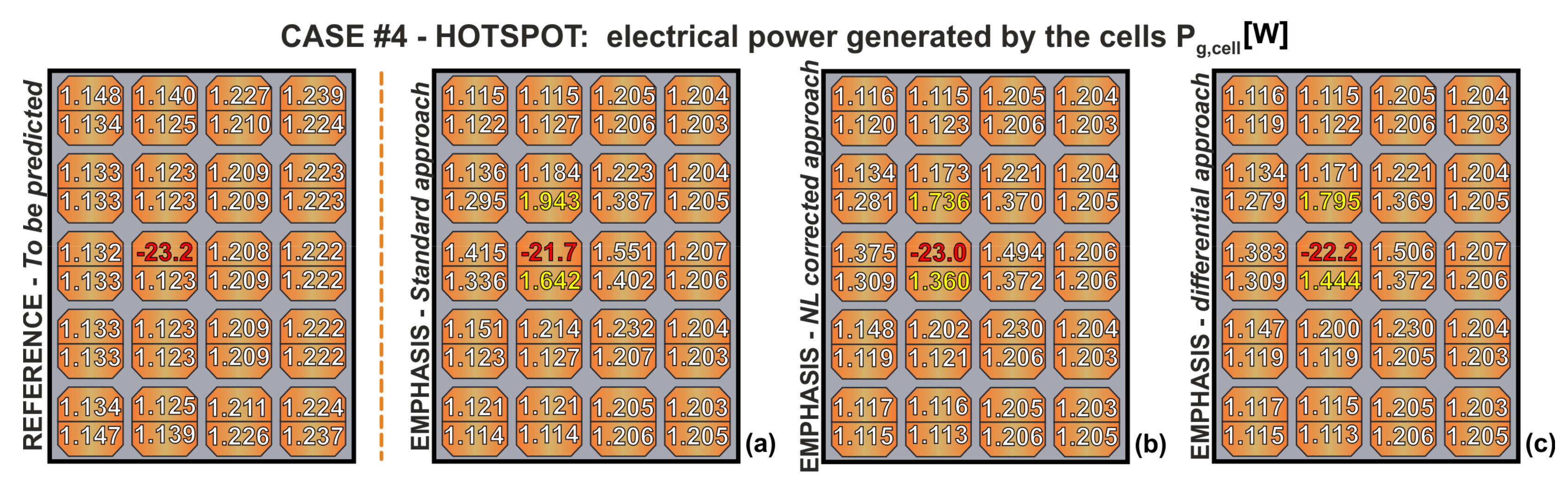
In the HOTSPOT case, instead, a significant temperature increment was observed in proximity of the shaded cell (Figure 10d). In addition, under these conditions, EMPHASIS successfully detected the localized malfunctions. Figure 13 states that the negative Pg,cell value corresponding to cell #5 was predicted, regardless of the adopted approach. In addition, the estimation of all the remaining Pg,cell values is trustworthy, the only exception being the cells surrounding the partially shaded one. Because of the huge temperature increment of cell #5, these cells are characterized by strong temperature gradients, which lead to an overestimation of the absolute value of the—negative and ingoing—horizontal heat flux (i.e., Pout,i in Equation (3)). As a result, these Pg,cell values are slightly overestimated. However, EMPHASIS still identifies the cells surrounding the partially shaded one as correctly working (i.e., as generating electrical power). The main difference between the three approaches consists in the prediction of the power dissipated by the shaded cell. The standard approach leads to an error of ~6.5%, whereas the differential approach error was ~4.3%. The more complex calibration procedure of the NL-corrected approach is rewarded with improved predictions (error of ~0.9%); it can be inferred that—when high temperatures are observed—this approach can be successfully adopted to mitigate the error introduced by the NL thermal effects.
A comprehensive comparison between the approaches in the diagnosis of Cases #3 and #4 is reported in Table 2, which shows the subpanel- and panel-level electrical powers. In accordance with the cell-level discussion, no significant differences were found in the three approaches applied to the SHUNT case. EMPHASIS predicted the power generated by the subpanel (panel) with an absolute error lower than 0.5 W (1 W). With regard to the HOTSPOT case, the method was able to recognize the left subpanel—which includes the partially-shaded cell—as malfunctioning. The most accurate panel-level prediction was achieved by the NL-corrected approach that provided an absolute error of ~2 W. Concerning the differential approach, the calibration procedure relying on two temperature maps is conveniently traded for highly accurate results. By moving from the standard to the differential approach, the panel-level estimation error improves from 16.6% to 13.1%.
As a last result, a comparison between EMPHASIS and the methods previously presented in [40,41] is summarized in Table 3. The methodology shown in [40] corresponds to the early version of the standard approach, while the differential approach is an improvement of the method described in [41]. In the HOTSPOT case and regardless of the approach, EMPHASIS proved to be more precise than its previous versions with a significant reduction in the estimation errors of the electrical powers of both the malfunctioning cell and the panel electrical powers. The same can be inferred for the cell-level prediction in the SHUNT case, while the EMPHASIS panel-level estimation was found to be seemingly worse than the one achieved in [40]. However, since the method in [40] overestimates (underestimates) the cell- (panel-) level electrical powers, its better prediction is to be ascribed to compensation of the errors.
5. Conclusions
In this work, an Efficient Method for PHotovoltaic Arrays Study through Infrared Scanning (EMPHASIS) has been proposed and thoroughly described. EMPHASIS is an innovative analytical technique able to predict—on the basis of the mere knowledge of IR temperature maps—the cell-level working conditions of any PV panel. Moreover, the accuracy of the method predictions has been evaluated through a strategy relying on “simulated experiments,” which are not to be replicated by the EMPHASIS end users. A methodology has been conceived to feed the proposed method with numerical, yet realistic, temperature maps associated to a known power pattern, which has been compared to the one assessed by EMPHASIS.
The “simulated experiments” have been performed under realistic working conditions to emulate ad hoc localized malfunction events. EMPHASIS—in its three variants—has been applied on temperature maps of PV panels affected by a shunted cell and a localized hotspot. As a main result, an excellent agreement has been found and each variant has turned out to be reliable in the power assessment, with slight differences in terms of accuracy. In the case study concerning the PV panel with a shunted cell, EMPHASIS has provided negligible errors in the cell-level predictions; more specifically, the malfunctioning cell has been identified, and its reduced generated power has been correctly assessed. As far as the PV panel with a hotspot cell is concerned, the corresponding power loss has been quantified with an estimation error in the range of 9–16%. The whole investigation has witnessed that EMPHASIS can be successfully adopted to localize faults. In addition, the proposed method is expected to stand out among all other techniques presented in literature for being able to predict the actual cell- and panel-level electrical powers.
Author Contributions
Conceptualization, A.P.C., C.S., P.G., S.D. and V.d.A.; methodology, A.P.C., C.S., P.G., S.D. and V.d.A.; software, A.P.C., C.S. and P.G.; validation, A.P.C., C.S. and P.G.; formal analysis, A.P.C., C.S., P.G., S.D. and V.d.A; investigation, A.P.C., C.S., P.G., S.D. and V.d.A; resources, P.G.; writing—original draft preparation, A.P.C. and C.S.; writing—review and editing, A.P.C., C.S., P.G. and V.d.A.; supervision, V.d.A. All authors have read and agreed to the published version of the manuscript.
Funding
This research received no external funding.
Institutional Review Board Statement
Not applicable.
Informed Consent Statement
Not applicable.
Data Availability Statement
Not applicable.
Acknowledgments
The research activity of A.P.C. was supported by the University of Rome “Sapienza” through the scholarship named in memory of Francesco Paolo Califano. The funding for the Ph.D. activity of C.S. was generously donated by the Rinaldi family in the memory of Niccolò Rinaldi, a bright Professor and Researcher of University of Naples Federico II, prematurely passed away in 2018.
Conflicts of Interest
All authors declare no potential conflict of interest relevant to this article.
Nomenclature
| 2-D | Two-dimensional |
| 3-D | Three-dimensional |
| Acell | Cell area |
| Aglass | Panel front surface |
| Apixel | Pixel area |
| BC | Boundary condition |
| EMPHASIS | Efficient Method for PHotovoltaic Arrays Study through Infrared Scanning |
| ET | Electrothermal |
| EVA | Ethylene vinyl acetate |
| FEM | Finite-element method |
| G | Solar irradiance |
| Gexp | Experimental solar irradiance |
| hback | Heat transfer coefficients on the back surface |
| hfront | Heat transfer coefficients on the front surface |
| Iph | Photogenerated current |
| IR | Infrared |
| ISC | Short-circuit current |
| k | Thermal conductivity |
| MPP | Maximum-power-point |
| NL | Nonlinear |
| OC | Open-circuit |
| PD | Dissipated power |
| Pg,cell | Electrical power generated by the cell |
| Pg,panel | Electrical power generated by the panel |
| PV | Photovoltaic |
| ri | Tuning parameter |
| Rs | Series resistance |
| Rsh | Shunt resistance |
| RSMH | Cell self- and mutual-heating resistance |
| Si | Silicon |
| STC | Standard test conditions |
| T0 | Reference temperature in the FEM solver |
| Tamb | Ambient temperature |
| Tglass | Front surface temperature |
| tglass | Glass thickness |
| Ti | Pixel-level front surface temperature |
| VOC | Open-circuit voltage |
References
- Maycock, P.D. Photovoltaics: PV market update. In Renewable Energy World. 2005. Available online: https://inis.iaea.org/search/search.aspx?orig_q=RN:37002952 (accessed on 1 September 2020).
- Kurokawa, K.; Kato, K.; Ito, M.; Komoto, K.; Kichimi, T.; Sugihara, H. A cost analysis of very large scale PV (VLS-PV) system on the world deserts. Proceedings of IEEE Photovoltaic Specialists Conference, New Orleans, LA, USA, 19–24 May 2002; pp. 1672–1675. [Google Scholar]
- Shah, R.; Mithulananthan, N.; Lee, K.Y. Large-scale PV plant with a robust controller considering power oscillation damping. IEEE Trans. Energy Convers. 2012, 28, 106–116. [Google Scholar] [CrossRef]
- Shuchao, W.; Shengpeng, D.; Wei, H.; Jun, C.; Xicai, Z. Three-level agc for large-scale PV power plant with string inverters. In Proceedings of the IEEE International Conference on Power System Technology (POWERCON), Wollongong, Australia, 28 September–1 October 2016. [Google Scholar]
- Clement-Nyns, K.; Haesen, E.; Driesen, J. The impact of charging plug-in hybrid electric vehicles on a residential distribution grid. IEEE Trans. Power Syst. 2009, 25, 371–380. [Google Scholar] [CrossRef] [Green Version]
- Lawder, M.T.; Suthar, B.; Northrop, P.W.; De, S.; Hoff, C.M.; Leitermann, O.; Crow, M.L.; Santhanagopalan, S.; Subramanian, V.R. Battery energy storage system (BESS) and battery management system (BMS) for grid-scale applications. Proc. IEEE 2014, 102, 1014–1030. [Google Scholar] [CrossRef]
- Wang, G.; Ciobotaru, M.; Agelidis, V.G. Power smoothing of large solar PV plant using hybrid energy storage. IEEE Trans. Sustain. Energy 2014, 5, 834–842. [Google Scholar] [CrossRef]
- Kroposki, B.; Johnson, B.; Zhang, Y.; Gevorgian, V.; Denholm, P.; Hodge, B.M.; Hannegan, B. Achieving a 100% renewable grid: Operating electric power systems with extremely high levels of variable renewable energy. IEEE Power Energy Mag. 2017, 15, 61–73. [Google Scholar] [CrossRef]
- Beltran, H.; Bilbao, E.; Belenguer, E.; Etxeberria-Otadui, I.; Rodriguez, P. Evaluation of storage energy requirements for constant production in PV power plants. IEEE Trans. Ind. Electron. 2012, 60, 1225–1234. [Google Scholar] [CrossRef]
- Begum, S.; Banu, R.; Ahammed, G.A.; Parameshachari, B.D. Performance degradation issues of PV solar power plant. In Proceedings of the IEEE International Conference on Electrical Electronics, Communication, Computer, and Optimization Techniques (ICEECCOT), Karnataka, India, 15–16 December 2017; pp. 311–313. [Google Scholar]
- Livera, A.; Theristis, M.; Makrides, G.; Georghiou, G.E. Recent advances in failure diagnosis techniques based on performance data analysis for grid-connected photovoltaic systems. Renew. Energy 2019, 133, 126–143. [Google Scholar] [CrossRef]
- Xia, L.; Wen, Z.; Liao, K.; Chen, J.; Li, Q.; Luo, X. Unveiling the Failure Mechanism of Electrical Interconnection in Thermal-Aged PV Modules. IEEE Trans. Device Mater. Reliab. 2019, 20, 24–32. [Google Scholar] [CrossRef]
- Ebrahim, A.F.; Youssef, T.; Ahmed, S.M.W.; Elmasry, S.E.; Mohammed, O.A. Fault detection and compensation for a PV system grid tie inverter. In Proceedings of the IEEE North American Power Symposium (NAPS), Pullman, WA, USA, 7–9 September 2014. [Google Scholar]
- Khalil, M. Failure prediction of PV inverters under operational stresses. In Proceedings of the IEEE International Conference on Environment and Electrical Engineering and IEEE Industrial and Commercial Power Systems Europe (EEEIC/I&CPS Europe), Genoa, Italy, 11–14 June 2019. [Google Scholar]
- Brooks, A.E.; Cormode, D.; Cronin, A.D.; Kam-Lum, E. PV system power loss and module damage due to partial shade and bypass diode failure depend on cell behavior in reverse bias. Proceedings of IEEE 42nd Photovoltaic Specialist Conference (PVSC), New Orleans, LA, USA, 14–19 June 2015. [Google Scholar]
- Manganiello, P.; Balato, M.; Vitelli, M. A Survey on Mismatching and Aging of PV Modules: The Closed Loop. Ieee Trans. Ind. Electron. 2015, 62, 7276–7286. [Google Scholar] [CrossRef]
- Satpute, R.G.; Morey, S.B.; Shende, P.A.; Deshmukh, Y.B. Shunt Faults Analysis of Solar PV-Based AC Standalone System. Proceedings of International Conference on Innovative Trends and Advances in Engineering and Technology (ICITAET), Sheagon, India, 27–28 December 2019; pp. 73–78. [Google Scholar]
- Rossi, D.; Omaña, M.; Giaffreda, D.; Metra, C. Modeling and Detection of Hotspot in Shaded Photovoltaic Cells. IEEE Trans. Very Large Scale Integr. (Vlsi) Syst. 2015, 23, 1031–1039. [Google Scholar] [CrossRef] [Green Version]
- Daliento, S.; Chouder, A.; Guerriero, P.; Pavan, A.M.; Mellit, A.; Moeini, R.; Tricoli, P. Monitoring, diagnosis, and power forecasting for photovoltaic fields: A review. Int. J. Photoenergy 2017. [Google Scholar] [CrossRef]
- Stellbogen, D. Use of PV circuit simulation for fault detection in PV array fields. Proceedings of IEEE Photovoltaic Specialists Conference, Louisville, KY, USA, 10–14 May 1993; pp. 1302–1307. [Google Scholar]
- Haeberlin, H.; Beutler, C. Normalized representation of energy and power for analysis of performance and on-line error detection in PV-systems. In Proceedings of the European Photovoltaic Solar Energy Conference, Nice, France, 23–27 October 1995. [Google Scholar]
- Chouder, A.; Silvestre, S. Automatic supervision and fault detection of PV systems based on power losses analysis. Energy Convers. Manag. 2010, 51, 1929–1937. [Google Scholar] [CrossRef]
- Drews, A.; De Keizer, A.C.; Beyer, H.G.; Lorenz, E.; Betcke, J.; Van Sark, W.G.J.H.M.; Heydenreich, W.; Wiemken, E.; Stettler, S.; Toggweiler, P.; et al. Monitoring and remote failure detection of grid-connected PV systems based on satellite observations. Sol. Energy 2007, 81, 548–564. [Google Scholar] [CrossRef] [Green Version]
- Vergura, S.; Acciani, G.; Amoruso, V.; Patrono, G.E.; Vacca, F. Descriptive and inferential statistics for supervising and monitoring the operation of PV plants. Ieee Trans. Ind. Electron. 2009, 56, 4456–4464. [Google Scholar] [CrossRef]
- Guerriero, P.; Piegari, L.; Rizzo, R.; Daliento, S. Mismatch based diagnosis of PV fields relying on monitored string currents. Int. J. Photoenergy 2017. [Google Scholar] [CrossRef] [Green Version]
- Sánchez-Pacheco, F.J.; Sotorrío-Ruiz, P.J.; Heredia-Larrubia, J.R.; Pérez-Hidalgo, F.; Sidrach De Cardona, M. PLC-based PV plants smart monitoring system: Field measurements and uncertainty estimation. IEEE Trans. Instrum. Meas. 2014, 63, 2215–2222. [Google Scholar] [CrossRef]
- Guerriero, P.; Di Napoli, F.; Vallone, G.; d’Alessandro, V.; Daliento, S. Monitoring and diagnostics of PV plants by a wireless self-powered sensor for individual panels. IEEE J. Photovolt. 2016, 6, 286–294. [Google Scholar] [CrossRef]
- Bellezza Quater, P.; Grimaccia, F.; Leva, S.; Mussetta, M.; Aghaei, M. Light Unmanned Aerial Vehicles (UAVs) for cooperative inspection of PV plants. IEEE J. Photovolt. 2014, 4, 1107–1113. [Google Scholar] [CrossRef] [Green Version]
- Hu, Y.; Cao, W.; Ma, J.; Finney, S.J.; Li, D. Identifying PV module mismatch faults by a thermography-based temperature distribution analysis. IEEE Trans. Device Mater. Reliab. 2014, 14, 951–960. [Google Scholar] [CrossRef] [Green Version]
- Tsanakas, J.A.; Chrysostomou, D.; Botsaris, P.N.; Gasteratos, A. Fault diagnosis of photovoltaic modules through image processing and Canny edge detection on field thermographic measurements. Int. J. Sustain. Energy 2015, 34, 351–372. [Google Scholar] [CrossRef]
- Vergura, S.; Marino, F. Quantitative and computer-aided thermography-based diagnostics for PV devices: Part I—Framework. IEEE J. Photovolt. 2017, 7, 822–827. [Google Scholar] [CrossRef]
- Vergura, S.; Colaprico, M.; de Ruvo, M.F.; Marino, F. A quantitative and computer-aided thermography-based diagnostics for PV devices—Part II: Platform and results. IEEE J. Photovolt. 2017, 7, 237–243. [Google Scholar] [CrossRef]
- Aghaei, M.; Grimaccia, F.; Gonano, C.A.; Leva, S. Innovative automated control system for PV fields inspection and remote control. IEEE Trans. Ind. Electron. 2015, 62, 7287–7296. [Google Scholar] [CrossRef]
- Aghaei, M.; Gandelli, A.; Grimaccia, F.; Leva, S.; Zich, R.E. IR real-time analyses for PV system monitoring by digital image processing techniques. In Proceedings of the International Conference on Event-Based Control, Communication and Signal Processing (EBCCSP), Krakow, Poland, 17–19 June 2015. [Google Scholar]
- Dotenco, S.; Dalsass, M.; Winkler, L.; Würzner, T.; Brabec, C.; Maier, A.; Gallwitz, F. Automatic detection and analysis of photovoltaic modules in aerial infrared imagery. In Proceedings of the IEEE Winter Conference on Applications of Computer Vision (WACV), New York, NY, USA, 7–9 March 2016. [Google Scholar]
- Guerriero, P.; Di Napoli, F.; Daliento, S. Real time monitoring of solar fields with cost/revenue analysis of fault fixing. In Proceedings of the IEEE International Conference on Environment and Electrical Engineering (EEEIC), Florence, Italy, 7–10 June 2016. [Google Scholar]
- Chine, W.; Mellit, A.; Lughi, V.; Malek, A.; Sulligoi, G.; Massi Pavan, A. A novel fault diagnosis technique for photovoltaic systems based on artificial neural networks. Renew. Energy 2016, 90, 501–512. [Google Scholar] [CrossRef]
- Kim, I.-S. On-line fault detection algorithm of a photovoltaic system using wavelet transform. Sol. Energy 2016, 126, 137–145. [Google Scholar] [CrossRef]
- Karatepe, E.; Hiyama, T. Controlling of artificial neural network for fault diagnosis of photovoltaic array. Proceedings of IEEE International Conference on Intelligent System Applications to Power Systems (ISAP), Hersonissos, Greece, 25–28 September 2011. [Google Scholar]
- Catalano, A.P.; Guerriero, P.; d’Alessandro, V.; Codecasa, L.; Daliento, S. An approach to the cell-level diagnosis of malfunctioning events in PV panels from aerial thermal maps. In ELECTRIMACS 2019 Selected Papers-Volume 2; Springer: Cham, Switzerland, 2020; p. 697, (Lecture Notes in Electrical Engineering). [Google Scholar]
- Guerriero, P.; Catalano, A.P.; Matacena, I.; Codecasa, L.; d’Alessandro, V.; Daliento, S. Experimental assessment of malfunction events in photovoltaic modules from IR thermal maps. In Proceedings of the IEEE International Workshop on Thermal Investigations of ICs and Systems (THERMINIC), Lecco, Italy, 25–27 September 2019. [Google Scholar]
- ET-M54050. Available online: http://www.etsolar.com.ar/folletos/ET-M54050(50w).pdf (accessed on 1 September 2020).
- Fluke TiS55 Infrared Camera. Available online: https://www.fluke.com/en-us/product/thermal-cameras/tis55# (accessed on 4 September 2020).
- PSPICE User’s Manual, Cadence OrCAD 16.5. 2011. Available online: https://www.seas.upenn.edu/~jan/spice/PSpice_CaptureGuideOrCAD.pdf (accessed on 4 September 2020).
- Guerriero, P.; Codecasa, L.; d’Alessandro, V.; Daliento, S. Dynamic electro-thermal modeling of solar cells and modules. Sol. Energy 2019, 179, 326–334. [Google Scholar] [CrossRef]
- Zekry, A.; Al-Mazroo, A.Y. A distributed SPICE-model of a solar cell. IEEE Trans. Electron Devices 1996, 43, 691–700. [Google Scholar] [CrossRef]
- d’Alessandro, V.; Catalano, A.P.; Codecasa, L.; Moser, B.; Zampardi, P.J. Modeling thermal coupling in bipolar power amplifiers toward dynamic electrothermal simulation. In Proceedings of the IEEE MTT-S International Conference on Numerical Electromagnetic and Multiphysics Modeling and Optimization (NEMO), Reykjavik, Iceland, 8–10 August 2018. [Google Scholar]
- d’Alessandro, V.; Catalano, A.P.; Codecasa, L.; Moser, B.; Zampardi, P.J. Combined SPICE-FEM analysis of electrothermal effects in InGaP/GaAs HBT devices and arrays for handset applications. In Proceedings of the IEEE International Conference on Thermal, Mechanical and Multi-Physics Simulation and Experiments in Microelectronics and Microsystems (EuroSimE), Toulouse, France, 16–18 April 2019. [Google Scholar]
- COMSOL Multiphysics, User’s Guide, Release 5.3A. 2018. Available online: https://cdn.comsol.com/doc/5.3a/COMSOL_ReleaseNotes.pdf (accessed on 1 September 2020).
- d’Alessandro, V.; Catalano, A.P.; Codecasa, L.; Zampardi, P.J.; Moser, B. Accurate and efficient analysis of the upward heat flow in InGaP/GaAs HBTs through an automated FEM-based tool and Design of Experiments. Int. J. Numer. Model. Electron. Netw. Devices Fields 2019, 32, e2530. [Google Scholar] [CrossRef]
- Catalano, A.P.; Scognamillo, C.; d’Alessandro, V.; Castellazzi, A. Numerical analysis and analytical modeling of the thermal behavior of single-and double-sided cooled power modules. IEEE Trans. Compon. Packag. Manuf. Technol. 2020, 10, 1446–1453. [Google Scholar] [CrossRef]
- Catalano, A.P.; Magnani, A.; d’Alessandro, V.; Codecasa, L.; Rinaldi, N.; Moser, B.; Zampardi, P.J. Numerical analysis of the thermal behavior sensitivity to technology parameters and operating conditions in InGaP/GaAs HBTs. Proceedings of IEEE the Compound Semiconductor Integrated Circuit Symposium (CSICS), Miami, FL, USA, 22–25 October 2017. [Google Scholar]
- Armstrong, S.; Hurley, W.G. A thermal model for photovoltaic panels under varying atmospheric conditions. Appl. Therm. Eng. 2010, 30, 1488–1495. [Google Scholar] [CrossRef]
- Lienhard, J.H., IV; Lienhard, J.H., V. A Heat Transfer Textbook; Phlogiston Press: Cambridge, MA, USA, 2008. [Google Scholar]
- Catalano, A.P.; d’Alessandro, V.; Guerriero, P.; Daliento, S. Diagnosis of power losses in PV plants by means of UAV thermography. In Proceedings of the IEEE International Conference on Clean Electrical Power (ICCEP), Otranto, Italy, 2–4 July 2019; pp. 306–310.
- Palankovski, W.; Quay, R. Analysis and Simulation of Heterostructure Devices; Springer: New York, NY, USA, 2004. [Google Scholar]
Figure 1.
Schematic representation of the EMPHASIS workflow illustrating the calibration procedure and the power estimation stages. The equation numbers are related to the standard approach (i.e., the first variant of EMPHASIS) presented in Section 2.1.
Figure 1.
Schematic representation of the EMPHASIS workflow illustrating the calibration procedure and the power estimation stages. The equation numbers are related to the standard approach (i.e., the first variant of EMPHASIS) presented in Section 2.1.

Figure 2.
Schematic depiction of the PV panel under investigation showing (i) the cells shape and numbering, (ii) the power terminals of the panel (Vpanel+ and Vpanel-), (iii) the electrical connections between cells (red dashed line), and (iv) the left and right subpanels.
Figure 2.
Schematic depiction of the PV panel under investigation showing (i) the cells shape and numbering, (ii) the power terminals of the panel (Vpanel+ and Vpanel-), (iii) the electrical connections between cells (red dashed line), and (iv) the left and right subpanels.
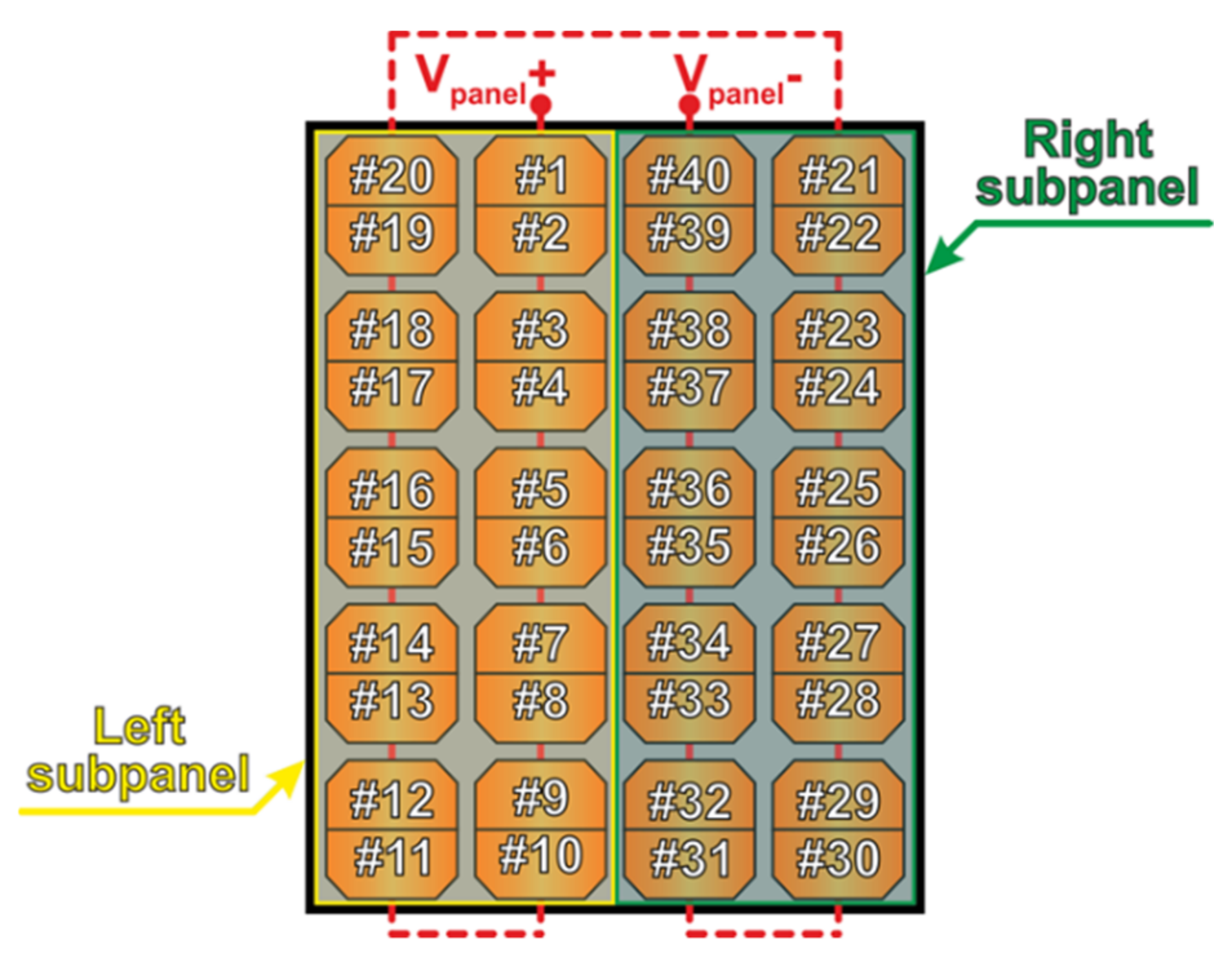
Figure 3.
Schematic 3-D representation (not to scale) of the PV panel technology illustrating materials and thickness of each layer composing the structure.
Figure 3.
Schematic 3-D representation (not to scale) of the PV panel technology illustrating materials and thickness of each layer composing the structure.

Figure 4.
Experimental temperature map of the panel under OC conditions obtained through IR scanning.
Figure 4.
Experimental temperature map of the panel under OC conditions obtained through IR scanning.
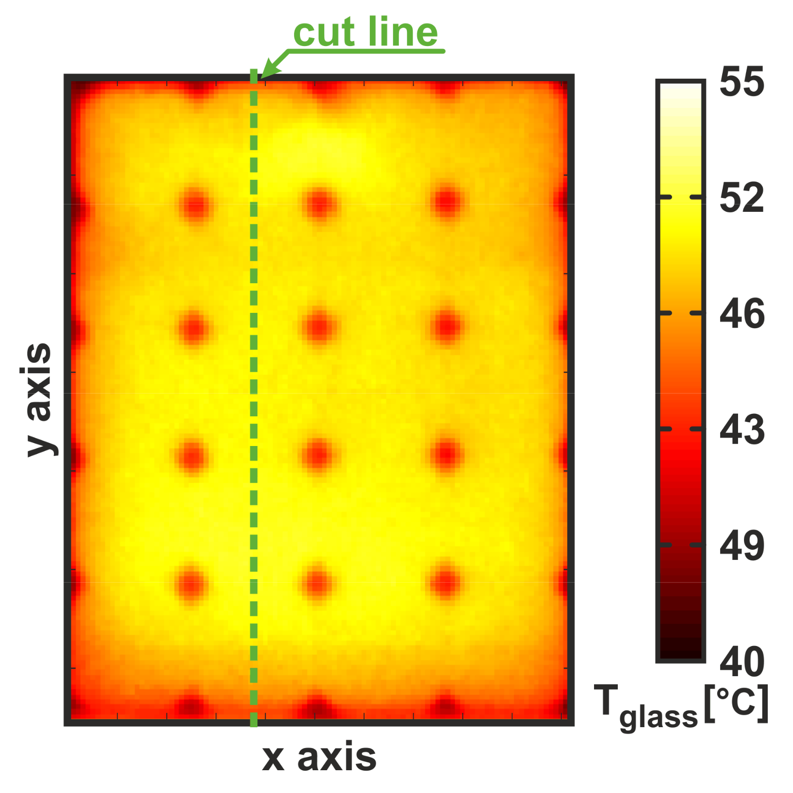
Figure 5.
ET cell subcircuit reporting the electrical behavioral model (left) and the corresponding thermal feedback circuit (right) based on the thermal equivalent of the Ohm’s law.
Figure 5.
ET cell subcircuit reporting the electrical behavioral model (left) and the corresponding thermal feedback circuit (right) based on the thermal equivalent of the Ohm’s law.
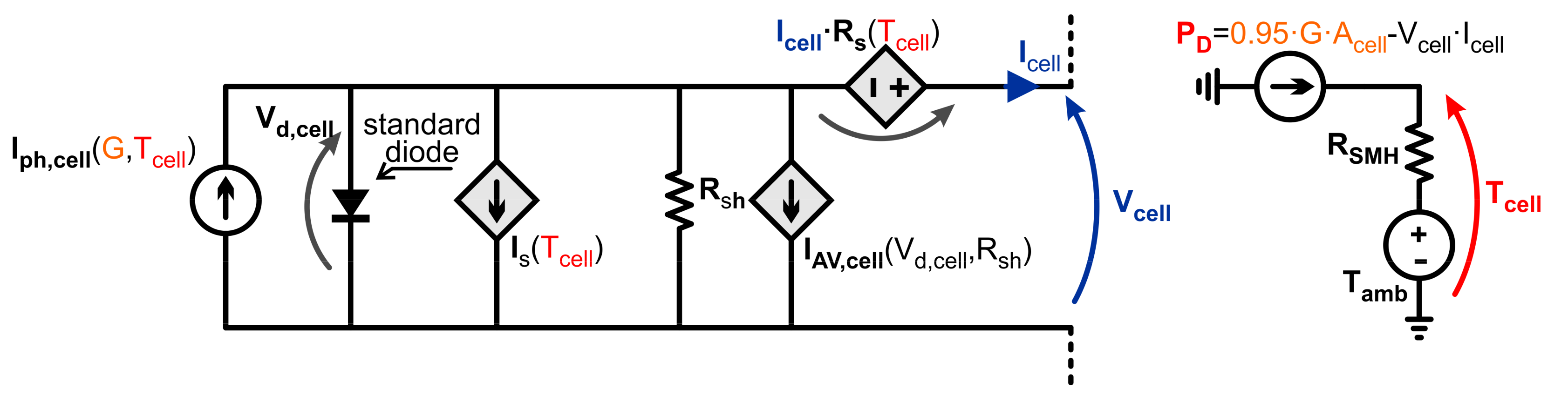
Figure 6.
Screenshot of the PV panel macrocircuit implemented in the SPICE-like environment; each of the 40 series-connected boxes contains the subcircuit shown in Figure 5. For illustrative purposes, the two Si-based bypass diodes were hidden.
Figure 6.
Screenshot of the PV panel macrocircuit implemented in the SPICE-like environment; each of the 40 series-connected boxes contains the subcircuit shown in Figure 5. For illustrative purposes, the two Si-based bypass diodes were hidden.
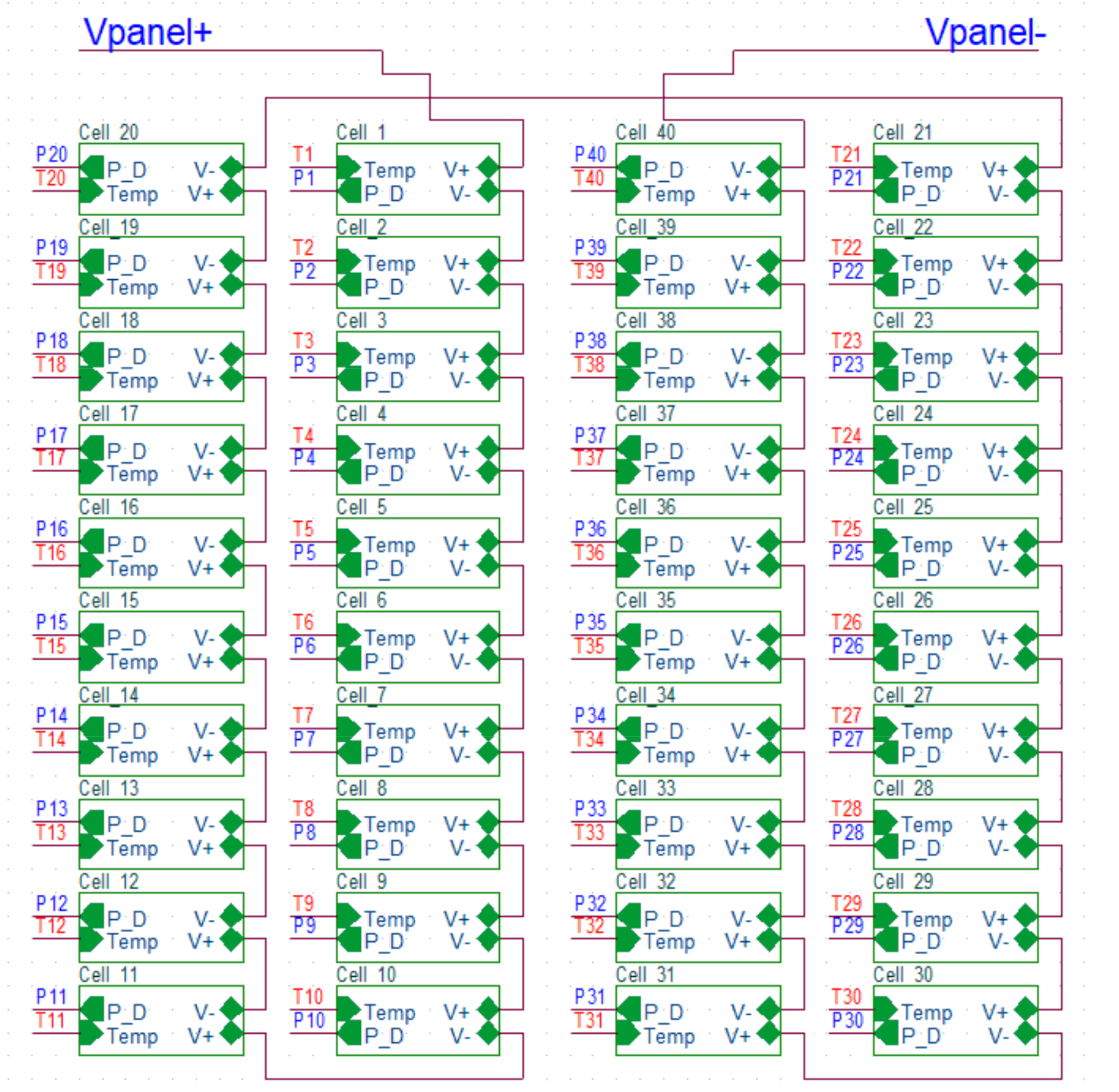
Figure 7.
3-D representations of the PV panel built in the COMSOL Multiphysics environment. The geometry, the tetrahedral mesh, and the solution of the thermal problem are reported in (a–c), respectively. Below the dashed lines, the glass layer is set as transparent to show the PV cells underneath.
Figure 7.
3-D representations of the PV panel built in the COMSOL Multiphysics environment. The geometry, the tetrahedral mesh, and the solution of the thermal problem are reported in (a–c), respectively. Below the dashed lines, the glass layer is set as transparent to show the PV cells underneath.

Figure 8.
Tglass along the cut line shown in Figure 4. The experimental data (red curve) are compared with the COMSOL simulation results (blue); the error reported in the legend quantifies the mismatch between the two distributions.
Figure 8.
Tglass along the cut line shown in Figure 4. The experimental data (red curve) are compared with the COMSOL simulation results (blue); the error reported in the legend quantifies the mismatch between the two distributions.

Figure 9.
Cell electrical power Pg,cell obtained by means of the ET simulations in the OrCad environment; (a) MPP conditions (Case #1), (b) OC conditions (Case #2), (c) cell #34 shunted (Case #3, SHUNT), and (d) cell #5 partially shaded (Case #4, HOTSPOT). Both the shunted and shaded cells are highlighted in red.
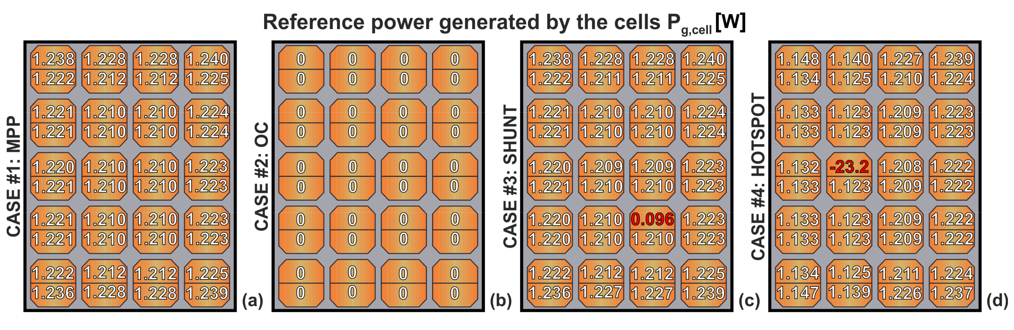
Figure 10.
Front surface pixel temperature Ti evaluated by the numerical simulations; (a) MPP conditions (Case #1), (b) OC conditions (Case #2), (c) cell #34 shunted (Case #3), and (d) cell #5 partially shaded (Case #4). The red dashed circle shows the slightly higher temperature of cell #34 in Case #3.
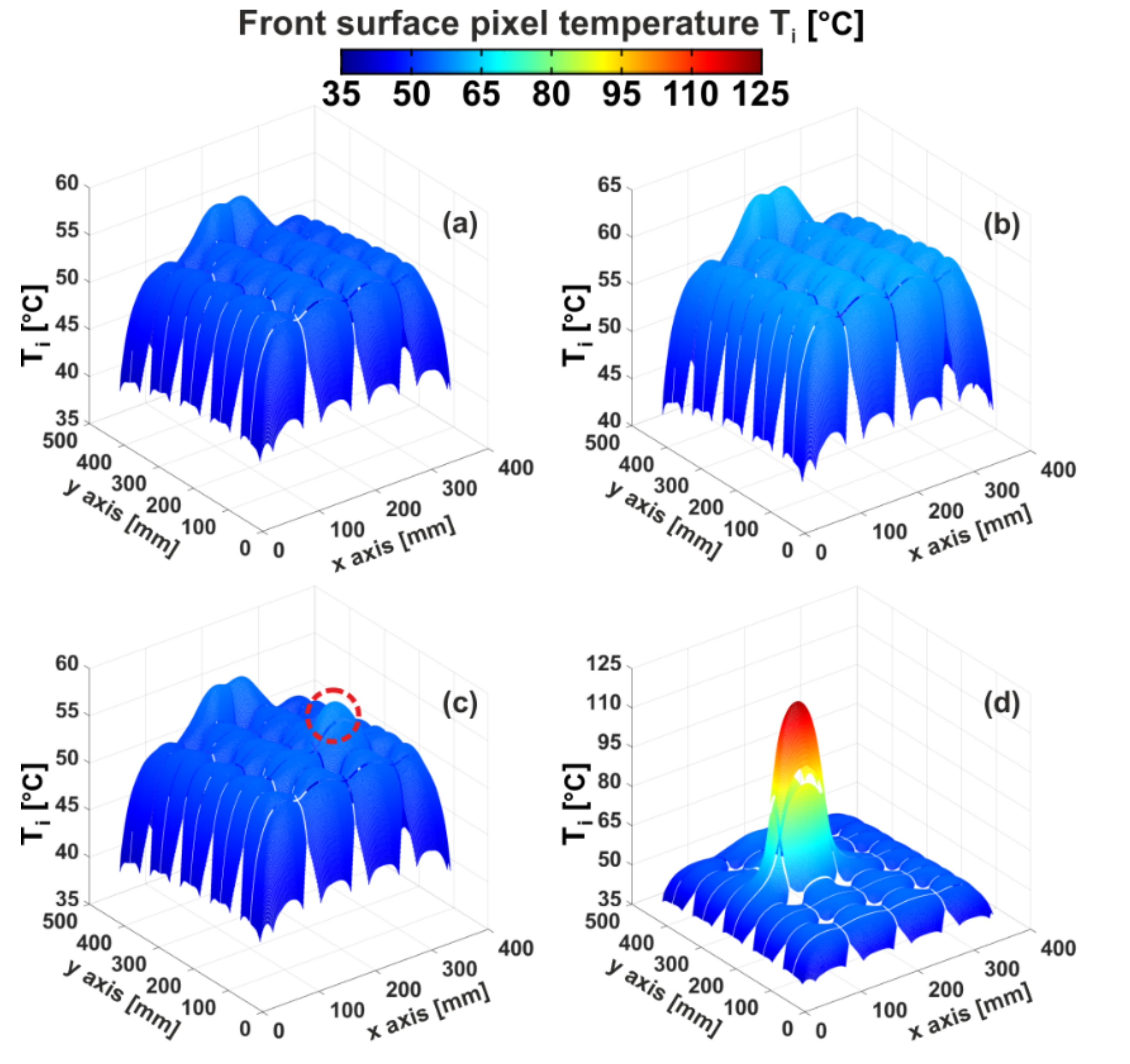
Figure 11.
The pixel outgoing thermal power Pout.i evaluated by applying Equation (2); (a) MPP conditions (Case #1), (b) OC conditions (Case #2), (c) cell #34 shunted (Case #3), and (d) cell #5 partially shaded (Case #4).
Figure 11.
The pixel outgoing thermal power Pout.i evaluated by applying Equation (2); (a) MPP conditions (Case #1), (b) OC conditions (Case #2), (c) cell #34 shunted (Case #3), and (d) cell #5 partially shaded (Case #4).
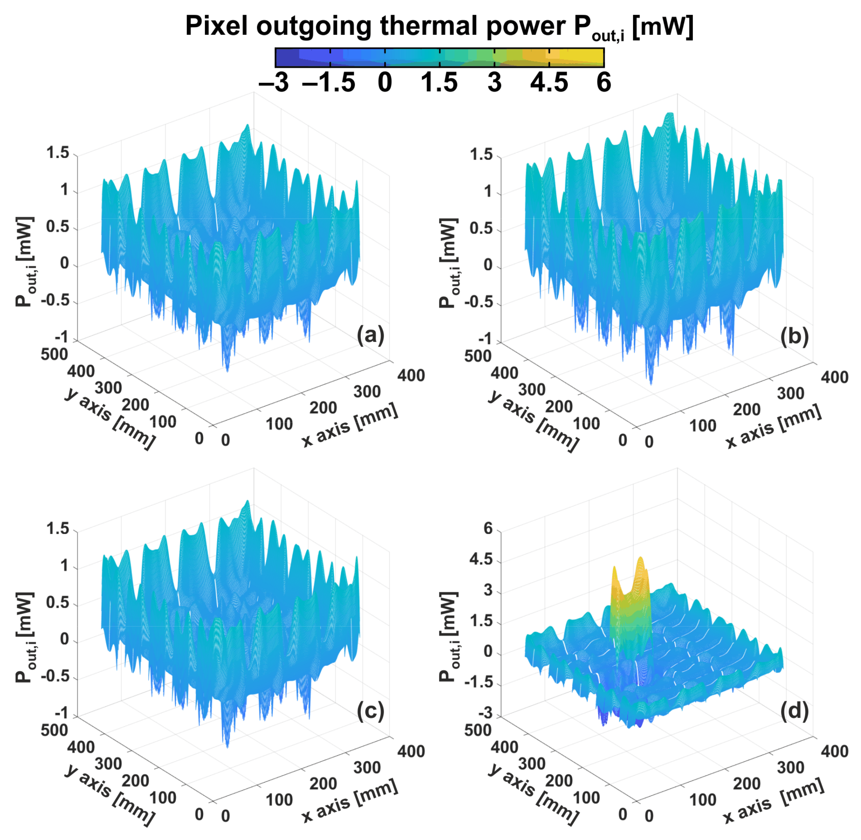
Figure 12.
Estimated electrical powers Pg,cells obtained in the SHUNT case study by means of EMPHASIS; (a) standard, (b) nonlinear (NL corrected), and (c) differential approach. The Pg,cell predicted values are to be compared with the reference ones shown on the left.
Figure 12.
Estimated electrical powers Pg,cells obtained in the SHUNT case study by means of EMPHASIS; (a) standard, (b) nonlinear (NL corrected), and (c) differential approach. The Pg,cell predicted values are to be compared with the reference ones shown on the left.
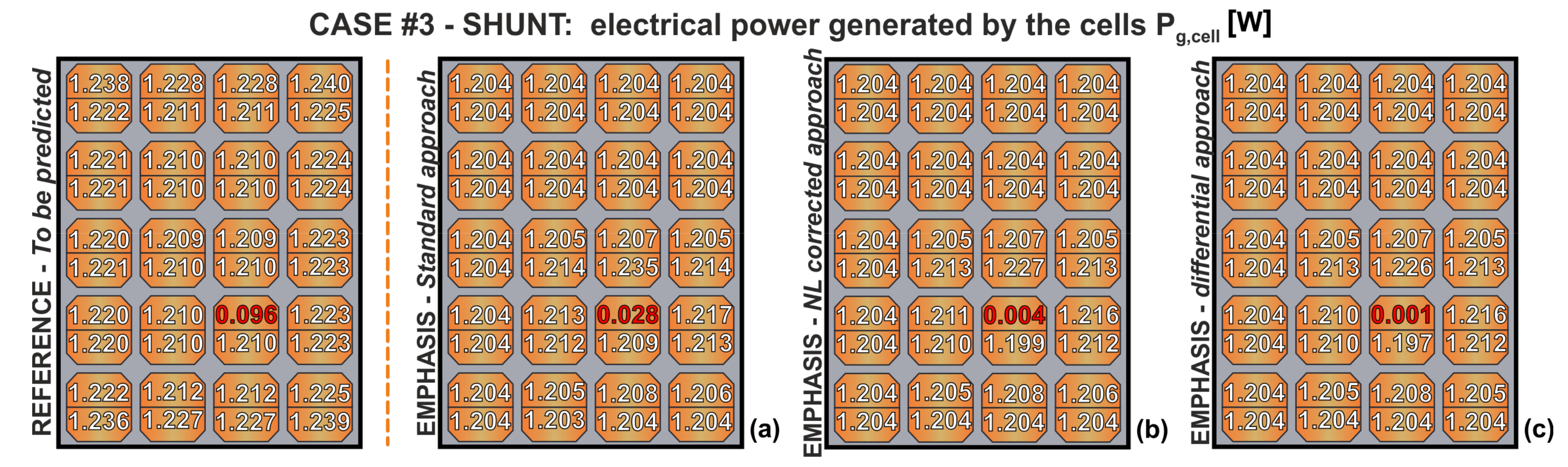
Figure 13.
Estimated electrical powers Pg,cells obtained in the HOTSPOT case study by means of EMPHASIS; (a) standard, (b) NL corrected, and (c) differential approach. The Pg,cell predicted values are to be compared with the reference ones shown on the left.
Figure 13.
Estimated electrical powers Pg,cells obtained in the HOTSPOT case study by means of EMPHASIS; (a) standard, (b) NL corrected, and (c) differential approach. The Pg,cell predicted values are to be compared with the reference ones shown on the left.

Table 1.
Thermal conductivities of the materials composing the PV panel under investigation.
| Material | k(T0) (W/mK) |
|---|---|
| Si | 148 [53] |
| Glass | 1.8 [53] |
| EVA | 0.35 [53] |
| Tedlar | 0.15 [53] |
| Aluminum | 237 [54] |
Table 2.
Summary of the subpanel- and panel-level electrical powers. The results are referred to the three EMPHASIS approaches applied on both the SHUNT and HOTSPOT cases; the mismatches with the reference power distributions are also reported.
Table 2.
Summary of the subpanel- and panel-level electrical powers. The results are referred to the three EMPHASIS approaches applied on both the SHUNT and HOTSPOT cases; the mismatches with the reference power distributions are also reported.
| Case #3—SHUNT | Case #4—HOTSPOT | |||||
|---|---|---|---|---|---|---|
| Left Subpanel | Right Subpanel | Whole Panel | Left Subpanel | Right Subpanel | Whole Panel | |
| Standard approach | 24.10 W (−0.38 W) | 22.98 W (−0.31 W) | 47.09 W (−0.58 W) | 1.52 W (+3.27 W) | 24.86 W (+0.47 W) | 26.38 W (+3.75 W) |
| NL-corrected approach | 24.10 W (−0.38 W) | 22.93 W (−0.36 W) | 47.03 W (−0.64 W) | −0.08 W (+1.68 W) | 24.76 W (+0.37 W) | 24.67 W (+2.04 W) |
| Differential approach | 24.10 W (−0.38 W) | 22.93 W (−0.36 W) | 47.03 W (−0.64 W) | 0.83 W (+2.6 W) | 24.77 W (+0.38 W) | 25.59 W (+2.96 W) |
| Reference | 24.38 W | 23.29 W | 47.67 W | −1.75 W | 24.39 W | 22.63 W |
Table 3.
Estimation error in the prediction of the malfunctioning cell and panel-level electrical powers in SHUNT and HOTSPOT cases; comparison between EMPHASIS and the methods presented in [40,41].
| SHUNT Case | HOTSPOT Case | |||
|---|---|---|---|---|
| Malfunctioning Cell Error | Panel-Level Error | Malfunctioning Cell Error | Panel-Level Error | |
| Method in [40] | +0.15 W | −0.45 W | −5.77 W | +4.38 W |
| EMPHASIS standard approach | −0.07 W | −0.58 W | −1.52 W | +3.75 W |
| Method in [41] | – | – | +9.27 W | +9.81 W |
| EMPHASIS differential approach | – | – | +1.01 W | +2.04 W |
Publisher’s Note: MDPI stays neutral with regard to jurisdictional claims in published maps and institutional affiliations. |
© 2021 by the authors. Licensee MDPI, Basel, Switzerland. This article is an open access article distributed under the terms and conditions of the Creative Commons Attribution (CC BY) license (http://creativecommons.org/licenses/by/4.0/).
Share and Cite
MDPI and ACS Style
Catalano, A.P.; Scognamillo, C.; Guerriero, P.; Daliento, S.; d’Alessandro, V. Using EMPHASIS for the Thermography-Based Fault Detection in Photovoltaic Plants. Energies 2021, 14, 1559. https://doi.org/10.3390/en14061559
AMA Style
Catalano AP, Scognamillo C, Guerriero P, Daliento S, d’Alessandro V. Using EMPHASIS for the Thermography-Based Fault Detection in Photovoltaic Plants. Energies. 2021; 14(6):1559. https://doi.org/10.3390/en14061559
Chicago/Turabian StyleCatalano, Antonio Pio, Ciro Scognamillo, Pierluigi Guerriero, Santolo Daliento, and Vincenzo d’Alessandro. 2021. "Using EMPHASIS for the Thermography-Based Fault Detection in Photovoltaic Plants" Energies 14, no. 6: 1559. https://doi.org/10.3390/en14061559
Note that from the first issue of 2016, this journal uses article numbers instead of page numbers. See further details here.