1. Introduction and Motivation
Nowadays, one of the major challenges for the automotive industry is the development of the fully autonomous vehicles, which is represented by level 5 of SAE J3016. This challenge involves several disciplines (e.g., sensing, controlling, decision making), which must work together to develop safe and reliable solutions for autonomous vehicles. One of the most significant tasks is the control design, because in the dynamics of the vehicle, it is highly nonlinear in its entire operation range. The nonlinear behavior becomes especially important at dangerous maneuvers (e.g., low road adhesion, high speed etc.), in which the vehicle is close to its physical limits.
Controlling of nonlinear system is still a challenging task, which draws attention from both engineers and researchers. In the past decades, several algorithms and control methods have been developed to deal with this problem. The developed approaches in two main categories can be classified: classical methods and machine learning-based solutions.
The classical methods includes the model-based control analysis and synthesis techniques, i.e., linear robust and optimal control methods (
), parameter-varying methods, e.g., Linear Parameter Varying (
LPV) and Nonlinear Parameter Varying (
NLPV) [
1,
2], Model Predictive Control (
MPC) approaches [
3] or polynomial methods [
4,
5]. One of the main sources of the nonlinearities is the tire-road contact, it stability is analyzed in [
6] and a Lyapunov control method for this problem is presented in [
7]. The uncertainties and the nonlinearities of the vehicle may have external sources, which can be handled by an adaptive robust controller, see [
8]. The steering system and its actuator also have nonlinearities, which can be controlled by an
LPV-based controller [
9]. The identification of the uncertainties and nonlinearities is also a challenging task. The authors of [
10] present a grey-box
LPV identification method for vehicles using side-slip angle estimation. An
LPV framework-based uncertainty identification is proposed in [
11] using experimental data.
These algorithms handle nonlinearities and unmodelled dynamics in the form of uncertainties and thus, they provide conservative solutions. Nevertheless, the result of the design is a control loop with guarantees on the stability and on the performances.
The machine-learning-based solutions include various methods, such as deep learning through the training of neural networks [
12], Support Vector Machine (
SVM), or decision logic algorithms [
13,
14,
15]. The main advantage of these algorithms is that they can learn from data, thus their models inherently contain the nonlinear behavior of the control plant. Thus, in several control applications, better performances comparing to the classical approaches might be provided. However, some of these methods, especially the neural networks, have the drawback that it is difficult to find systematic methods to prove the stability and performances of the closed-loop system. Since autonomous vehicles are safety-critic systems, it is recommended to reformulate the learning problem.
There are other solutions that deal with the identification problem of the dynamical systems. For example, in [
16,
17]
SVM-LS-based
LPV system identification methods are presented. Another data-driven identification solution can be found in [
18], which can ease the tuning of the hyperparameters of the model identification process. A non-parametric and probabilistic approach is proposed by [
19] for identifying nonlinear system considering uncertain noises on the measured signals. particle Bernstein polynomials-based regression method is presented in [
20], which is suitable for multivariate regression problems.
In the literature, some solutions can be found, which can provide methods for the reformulation of the learning features in the control problem. For example, [
21] proposes a
MPC-based control solution, in which the terminal cost and set are determined through an iterative process. In this idea, the model of the system is based on physical principles with its limitations. Another solution is the Model Free Control (
MFC), which is proposed in [
22,
23]. The
MFC method does not require a model of the controlled system, but it uses a local model, in which the model of each time step is updated.
The goal of this paper is to reformulate the design of vehicle path tracking functionality as a modeling problem with learning features and a control design problem using a model-based approach. The main contribution of the paper is a novel identification method, by which an LPV model of the nonlinear system can be determined. Moreover, the selection of the scheduling parameters of the LPV system is determined by a machine-learning-based pace regression algorithm in the modeling process of the system. In this way, the performances of the LPV controller are enhanced, while the stability of the closed-loop system is also preserved. The efficiency and the operation of the proposed control algorithm is validated by a complex test scenario, which is performed in the high-fidelity simulation software, CarSim.
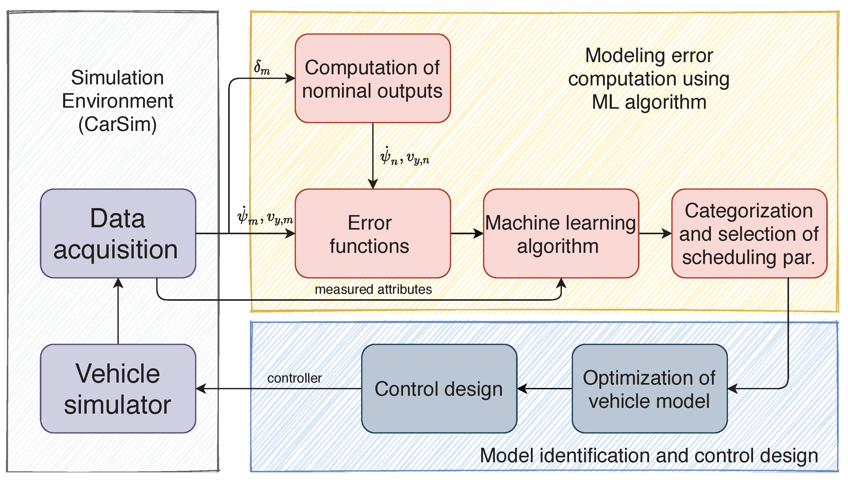
The process of the proposed method for achieving an enhanced vehicle control system is presented in
Figure 1. The process consists of three main layers with several tasks, i.e.,
Simulation environment,
Modeling error computation using ML algorithm and
Model identification and control design. Layer
Simulation environment consists of two tasks, namely, performing vehicle dynamic simulations for data generation and data acquisition. The vehicle dynamic simulations are performed on the high-fidelity simulation environment CarSim. The layer
Modeling error computation using ML algorithm consists of several tasks. It contains the selection and categorization of the scheduling parameters using the pace regression algorithm. It provides the categorized datasets for the identification process. The
Model identification and control design uses the categorized datasets for computing the models for each grid points of the
LPV system. In this layer, the
LPV-based control design is also presented, which guarantees the trajectory tracking of the vehicle.
In the paper, each layer and task are presented as follows.
Section 2 presents the vehicle model parameter tuning method for achieving control-oriented
LPV model. The control design based on the robust
LPV synthesis method is proposed in
Section 4. The effectiveness of the resulting control system through comparative simulation scenarios is examined in
Section 5. Finally, the achievements of the paper are concluded in
Section 6.
2. Formulation of the Control-Oriented LPV Model Using Data-Driven Approach
In this section, the data acquisition and the LPV-based data-driven model parameter tuning process are presented. Firstly, the collection of the dataset with numerous elements is detailed, which is provided by the vehicle dynamics simulation software, CarSim. Secondly, the prepocess of the collected data is explained, which includes the selection and the scaling of the data. Finally, the data-driven LPV-based model parameter tuning process is presented, in which the scheduling parameters and the model parameters are selected through a machine-learning-based pace regression algorithm.
2.1. Acquisition of Data from Simulations
Since all of the machine learning methods require a large amount of data to provide satisfying results, the first the of the algorithm is the data acquisition. In this paper, the high-fidelity simulation software, CarSim is used to generate the datasets for the machine learning algorithm in the control-oriented model formulation process. Since an appropriate dataset must cover a wide range of the vehicle operation, several simulations have been performed on the simulation environment using different parameter sets. These parameter sets includes the longitudinal velocity profile, the maneuvers, which must be performed by the vehicle. The test scenarios included several different routes with sharp bends (e.g., Melbourne Formula (1) circuit), whose adhesion coefficient has also been modified during the simulations. The dataset also includes simulations, in which the vehicle loses its stability, in order to cover most of the possible situations that the vehicle can encounter.
During the simulations, the following variables have been measured and collected:
- (1)
longitudinal velocity ()
- (2)
angular velocity of the wheels (), ,
- (3)
steering angle ()
- (4)
yaw-rate ()
- (5)
accelerations (, )
- (6)
lateral velocity ().
- (7)
side-slips of the wheels (), .
Note that all of the collected signals are available from the onboard system of the vehicle except the lateral velocity () and the side-slip angles. These signals are only used in the model formulation process, but during the operation of the proposed control method they are not required. The sampling time of the variables has been set to s. In this way, a large dataset has been created, which consisted of more than 10 million instances.
2.2. Categorization of Instances
The goal of the parameter optimization process is to get a set of models which are stable, as a first step the instances in the dataset must be categorized by their stability. The stability of the instances have a high impact on the performances of the optimization process; thus, the unstable instances must be removed from the dataset [
24]. The separation of the stable/unstable instances using only the measured values is not straightforward task. There is no general solution for determining the stability of a measurement. However, for the automotive case, a criterion is proposed in [
25], which can be used to separate the instances according to the stability of the vehicle:
where
is a experimentally defined parameter.
This criterion is based on the linear bicycle model, which will be detailed in the followings (2). Briefly, it compares the measured side-slips angle of the front wheel
, to the linear model, in which that angle is computed as
. The inequality (
1) describes that the deviation of the measured instance from the linear region, which can be used to determine the stability of the vehicle. Using this criterion, the dataset can be divided into two categories:
represents the set of the instances, where the motion of the vehicle is approximated as stable. Similarly,
denotes the set consisting of the instances with the approximation of unstable vehicle motion.
After separating the instances, error functions are computed, which reflects on the nonlinear behavior of the vehicle. Basically, the error function describes the deviation between the nominal model and the measured variables. The nominal model, which is used in this paper, is the two-wheeled bicycle model. The model consists of the following three main equations, ref. [
26]:
where
are the distances between the CoG and the front, rear axes of the vehicle,
are the reduced cornering stiffness of the wheels,
denotes the yaw-rate,
is the slid-slip,
m is the mass of the car,
I represents the yaw-inertia,
are the side-slip of the wheels and the longitudinal and lateral velocities are denoted by
. The lateral vehicle model can be transformed into a state-space representation
whose state-vector consists of
and its control input is the steering angle
. Furthermore, the measured variables have a sampling time of
s, therefore the model is sampled by the same sampling time. Using the measured input signal
, the outputs of the discrete system are computed for each measurement point.
The labeling of the collected data is based on the deviation of the measured signals from the signals of the nominal system. In this process, the yaw-rate and the lateral velocities are involved, which are the independent states of the physical system. The labeling is based on the relative errors of the signals in time
, such as
where
and
denote the measured outputs while
and
are the outputs of the nominal system.
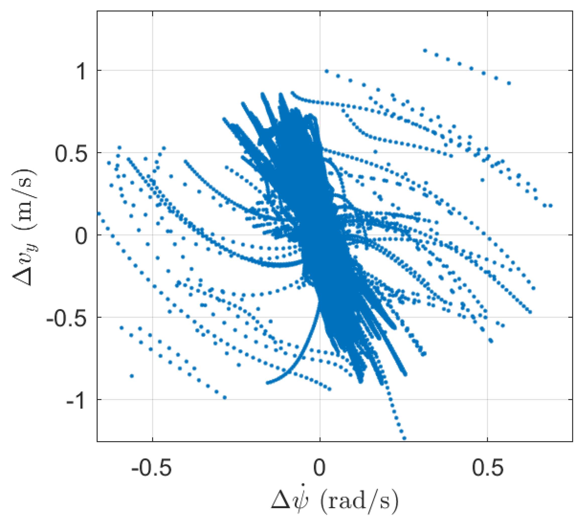
Figure 2 shows the function of
computed from the collected dataset.
Since neither nor are easy to calculate during the operation of the vehicle, a method must be found that is able to appropriately approximate the error signals using only the available measurements. In this paper the pace-regression algorithm is used for this purpose, which is briefly introduced in the following subsection.
4. Path Following LPV Control Design Using the Data-Driven Model
In this section, the
LPV-based lateral control design is presented. However, in some situations, the intervention is very limited using only the steering angle. It must be noted that, at specific operating points, the performance of the nominal intervention (steering angle) is limited due to the nonlinear dynamics of the vehicle. Therefore, the model is extended with the differential drive has a second input signal, which will be used to compensate the degraded performances of the steering system. This means that the model (2) is modified as:
where
denotes the differential torque. Moreover, the original model contains only two states: yaw-rate and the lateral velocity in order to simplify the optimization task by minimizing the number of the parameters. However, the lateral position tracking is also an important requirement for the autonomous vehicle, which can be computed from the existing states. Therefore, the state-space model is extended with at the lateral position
y, which can be computed as
at
tth s.
The identified system description is augmented as:
and
where the state vector of the system is
, the input is
.
The main goal of the control design is to guarantee the trajectory tracking of the vehicle, which can be achieved by describing performances for controller:
Minimization of the lateral error: As mentioned, the goal of the control design is to guarantee the trajectory tracking of the vehicle thus the error between the measured and the reference lateral positions must be minimized:
where is the reference lateral position computed from the track.
Minimization of the yaw-rate error: In order to achieve smooth trajectory tracking, a reference yaw-rate is also prescribed, which also must be tracked by the vehicle:
where
is the reference yaw-rate signal, computed from the curvature of the road, see [
26].
Minimization of the interventions: Due to the energy consumption, the interventions also must be minimized during the operation of the vehicle:
The performances are compressed into a performance-vector
, which leads to the following performance equation
where
are matrices and
r contains the reference signals
and
.
The basis of the control design is the presented data-driven
LPV model (
13), its measurement and performance equations are:
where (
19c) represents the measurement of
.
In order to guarantee the predefined performances ((
14)–(
16)), the system is augmented with several weighting functions. The augmented system is illustrated in
Figure 5. The weighting functions
aim to guarantee the tracking performances, while
aim to minimize the interventions. Since the parallel minimization of the performances and the interventions is contradictory, another goal of the weighting functions are to describe a balance between them.
and are used to scale the references signals (). Moreover, the role of the functions , is to attenuate the noises on the measured signals.
The goal of the control design is to find a
controller, which can guarantee the predefined performances and by which the closed-loop system is quadratically stable and its induced
norm is smaller than a
value. The optimization task can be formed as:
where
bounds the scheduling variables. The yielded controller
is formed as
where
,
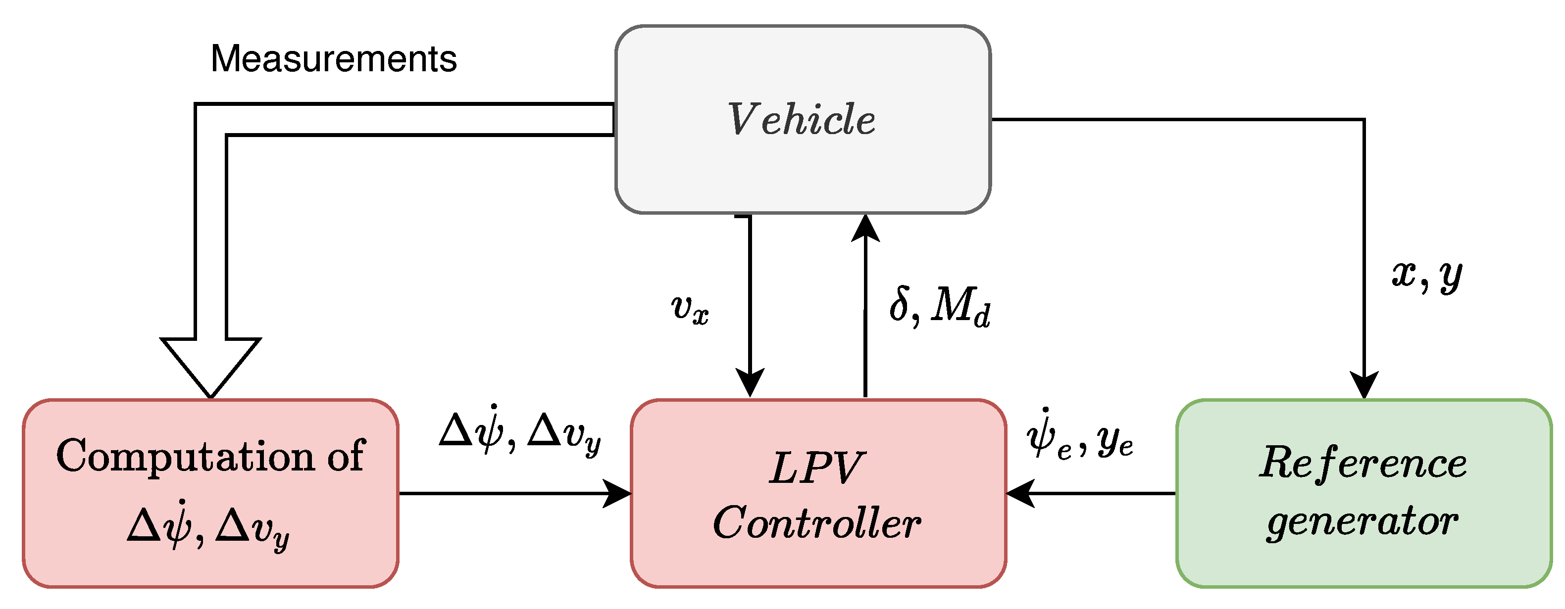
are variable-dependent matrices. The interconnected system is illustrated in
Figure 6 showing all of the main components of the proposed control system.
5. Simulation Results
In the followings, a complex test scenario is presented to show the efficiency and the operation of the proposed control algorithm in the high-fidelity vehicle dynamics simulation software, CarSim. In the simulations, the vehicle is driven along the Michigan Waterford hill track twice. In the first run, the vehicle is controlled by the proposed data-driven
LPV controller, while in the second turn, the car is driven by a nominal
LPV controller. Note that the nominal
LPV controller is tuned similarly to the proposed
LPV controller using the same number of weighting functions. However, the weights of the nominal
LPV controller are optimized to the nominal model presented in
Section 2.
The parameters of a car (e.g., mass, inertia, geometric attributes) are listed in
Table 1.
As presented in
Section 4, the
LPV controller contains several weighting functions, which aim to guarantee the predefined performances. The weighting functions of the reference signals are designed in such a way to ensure smooth trajectory tracking, while guaranteeing small tracking error:
The goal of the scaling functions
,
are to guarantee the trajectory tracking of the vehicle, they are designed by considering the maximal allowable errors, see:
The functions
and
aim to ensure the balance between the interventions and the tracking performances. As it can be seen, the weighting function belonging to the differential drive depends on the scheduling parameters
and
. It is tuned to compensate for the degraded performances of the steering system at the highly nonlinear region.
Finally, the weighting functions of the measurements are presented. They are used to attenuate the noises on the measured signals, which may have a negative effect on the performances.
In the followings, the results of the test scenarios are presented. As mentioned, the vehicle has been driven along the track twice. The track and the trajectories of the vehicle are illustrated in
Figure 7. As it can be seen, when the vehicle is controlled by the nominal
LPV controller, it leaves the road at a sharp bend. Whilst, in the second case, when the car is controlled by the proposed data-driven
LPV controller, it follows the road throughout the whole track.
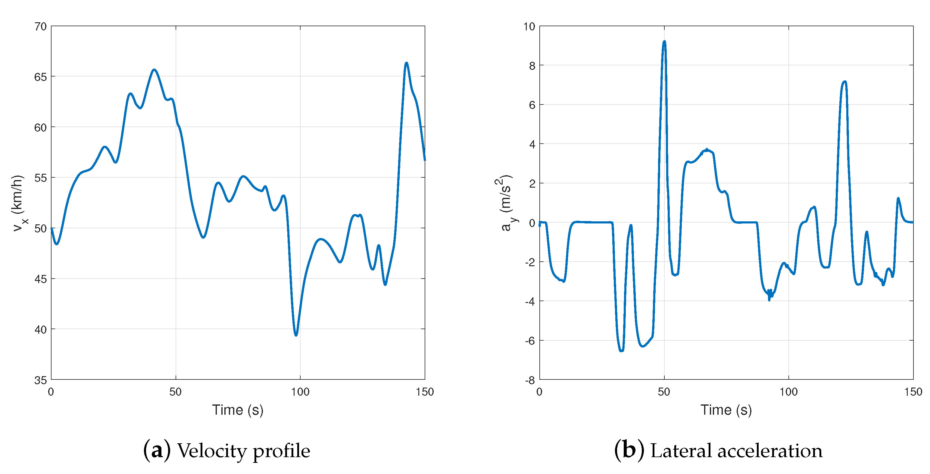
In order to show the operation of the proposed control method in a wide range, the longitudinal velocity of the vehicle varies between
<
> km/h, as shown in
Figure 8a.
Figure 8 demonstrates the lateral acceleration of the vehicle. As it can be seen, the maximum of the lateral acceleration is ≈10 m/s
, which means that the vehicle is close to its physical limits. This situation cannot be handled by the nominal controller; thus, the vehicle leaves the road.
Figure 9 shows the scheduling parameters and the yaw-rate tracking of the vehicle. As
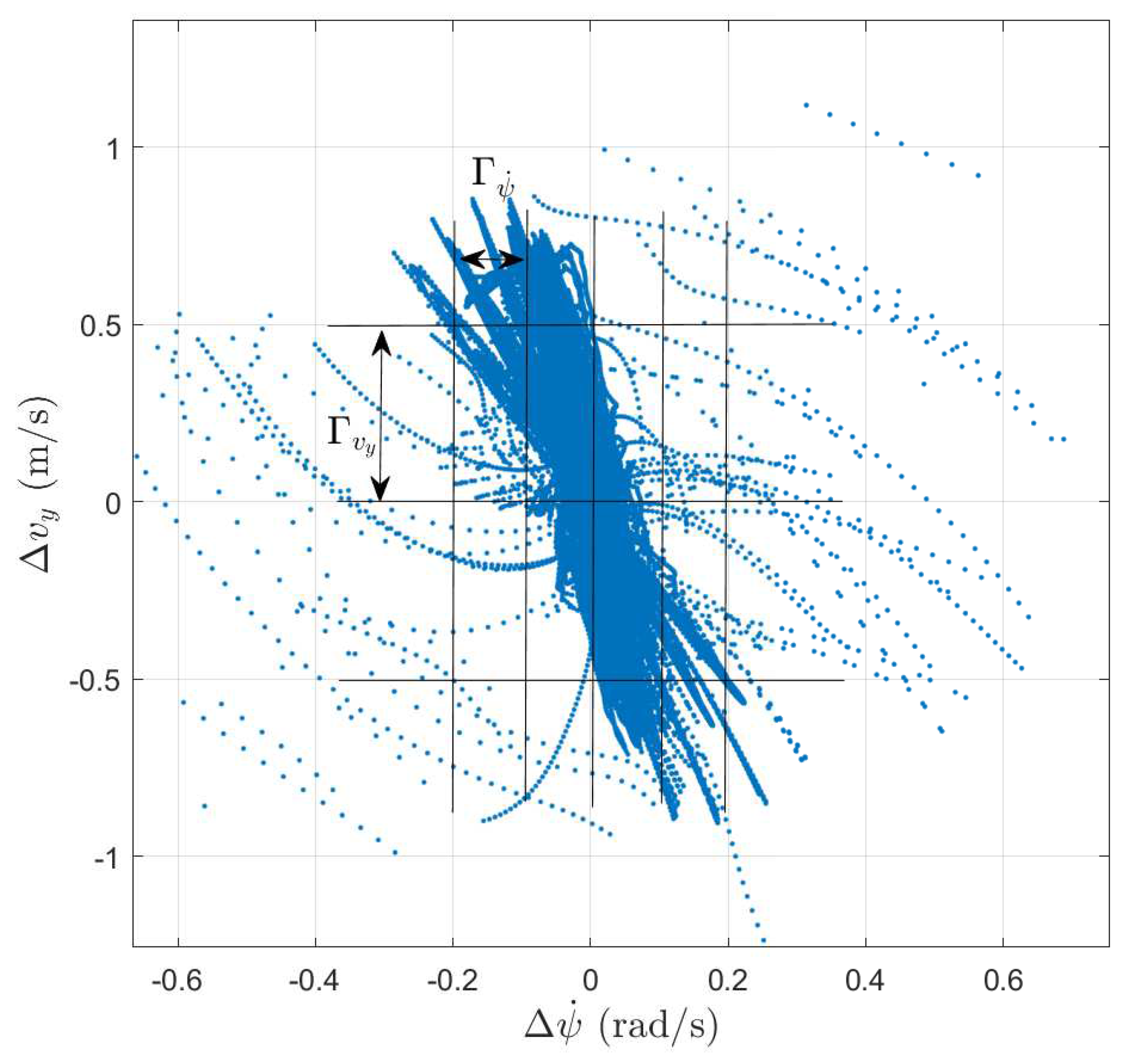
Figure 9a demonstrates, the scheduling parameters cover almost its whole range, as shown in
Figure 4. The yaw-rate tracking of the vehicle can be seen in
Figure 9b. The tracking is accurate the maximum error is only ≈0.02 rad/s. The yaw-rate signal varies in a wide range, its maximum is close to
rad/s, which is also close to the physical limits of the vehicle.
Finally, the interventions are illustrated in
Figure 10.
Figure 10a show the differential torque computed by the proposed control algorithm. As it can be seen, its maximal value is ≈600 Nm, which is provided at the sharp bend to compensate the steering angle. The steering angle is depicted in the right figure. It varies between
<
> rad, which is a reasonable range for the presented velocity profile.
