
Study of the Influence of the Lack of Contact in Plate and Fin and Tube Heat Exchanger on Heat Transfer Efficiency under Periodic Flow Conditions


Abstract
:
1. Introduction
2. Numerical Model of a Heat Exchanger
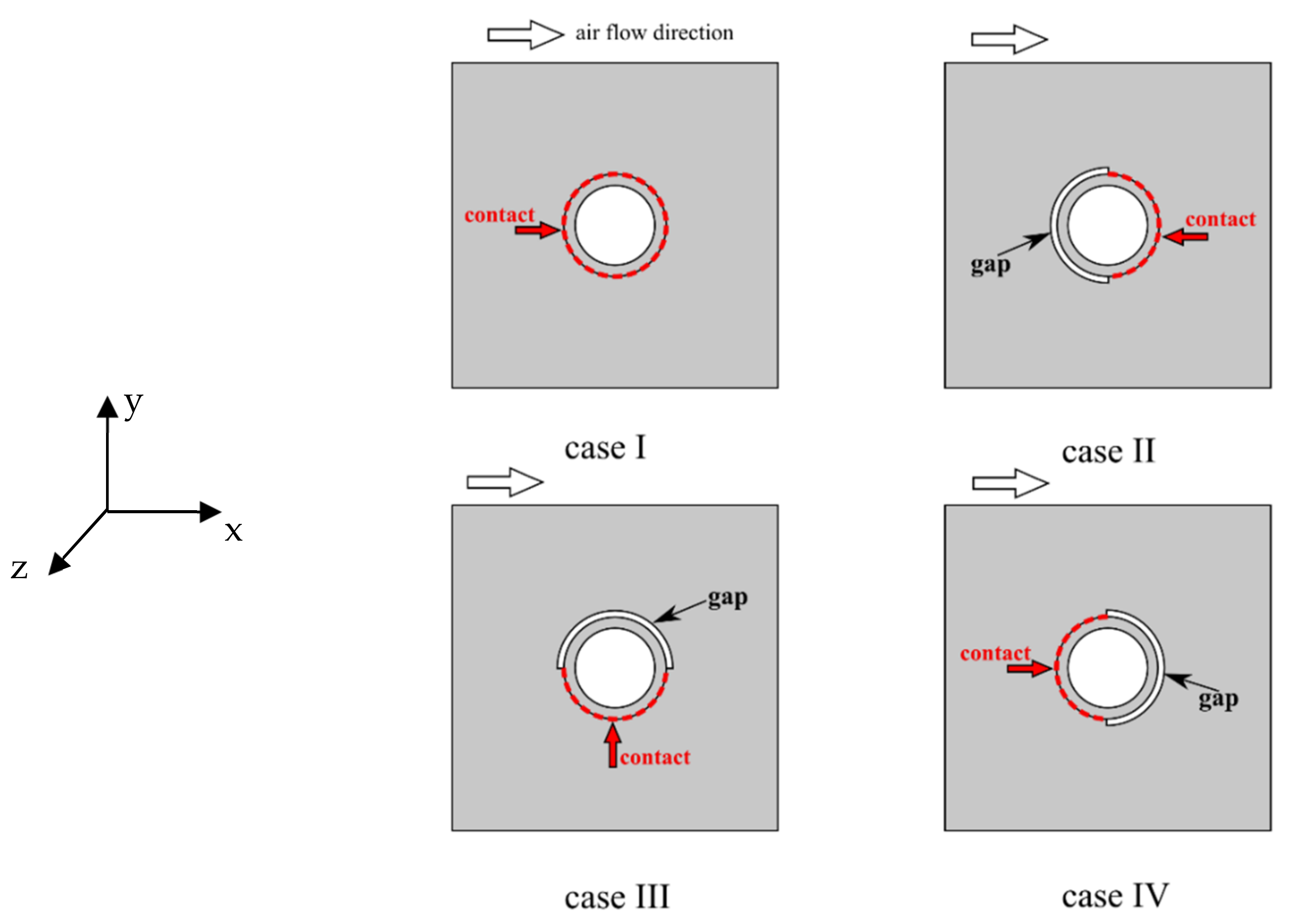
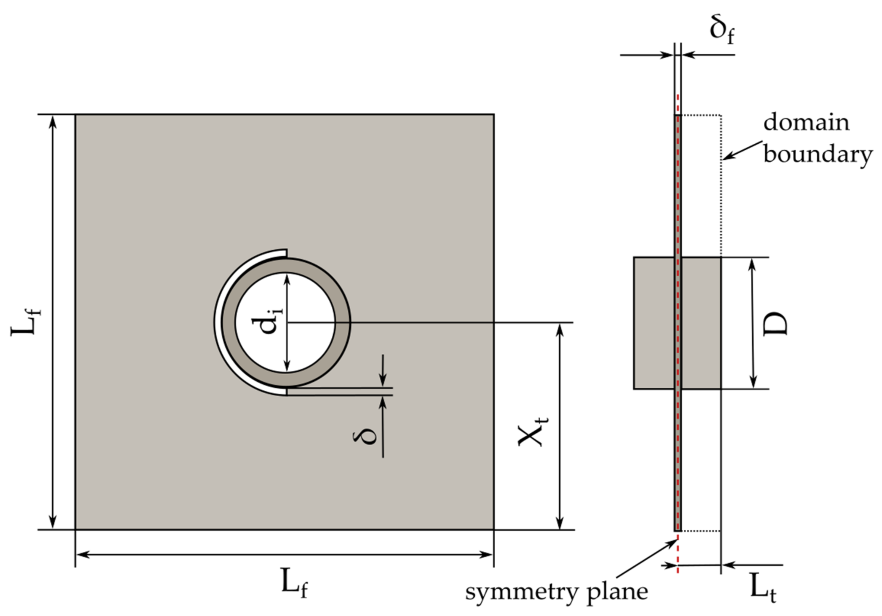
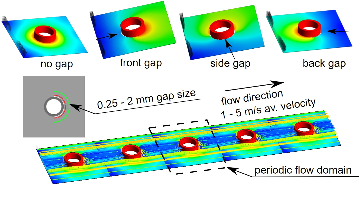
2.1. Geometry of the Computational Domain
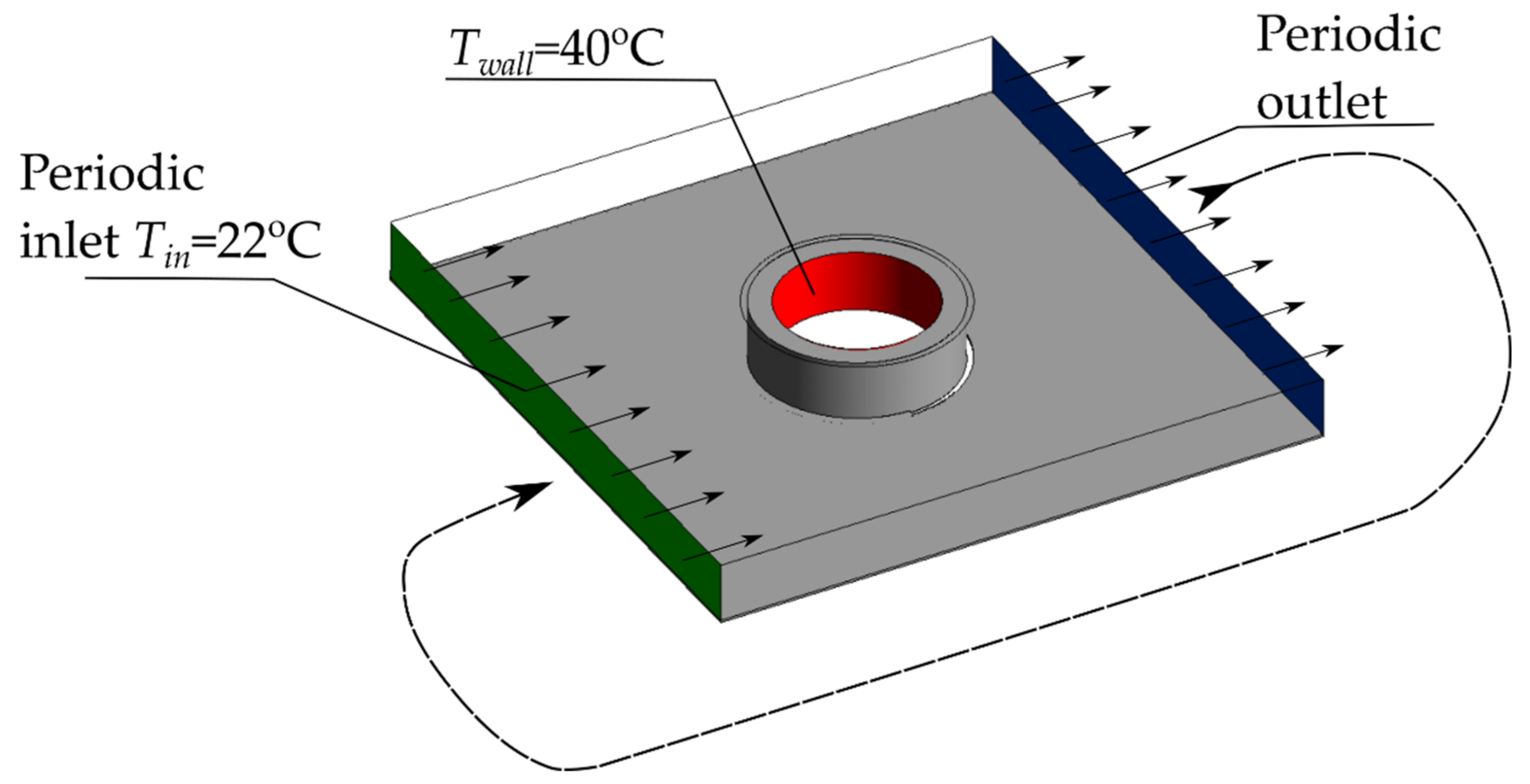
2.2. Boundary Conditions and Governing Equations
- Steady-state fluid flow and heat transfer;
- Fluid flow and heat transfer are periodic (fully-developed), meaning that pattern of flow/thermal solution has a periodically repeating nature (this condition is generally fulfilled for tube rows greater than the fourth row);
- Thermophysical properties of air are temperature-dependent (ideal gas);
- Natural convection was not considered as the highest Richardson number calculated for simulation conditions is Ri = (g·β·ΔT·L)/u2 = 0.025 (for Ri < 0.1 mechanism of natural convection can be typically considered negligible).
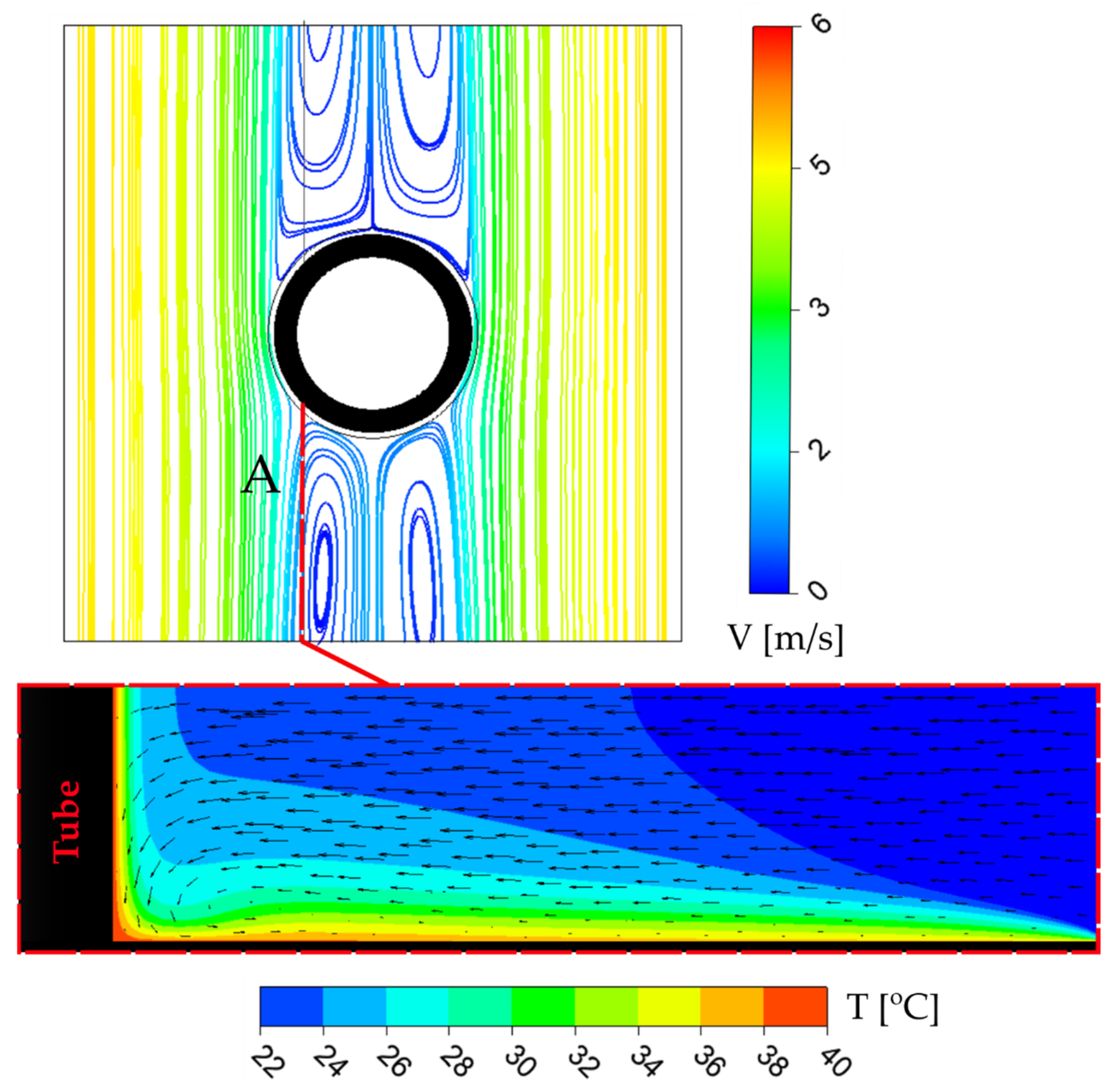
- Average air temperature at the inlet: Tave = 22 °C,
- u = 0 m/s on the fin and tube surfaces (no-slip condition),
- Uniform temperature at the inner surface of the tube wall: Tw = 40 °C—which corresponds to the condensation conditions of the working fluid flowing inside the tube.
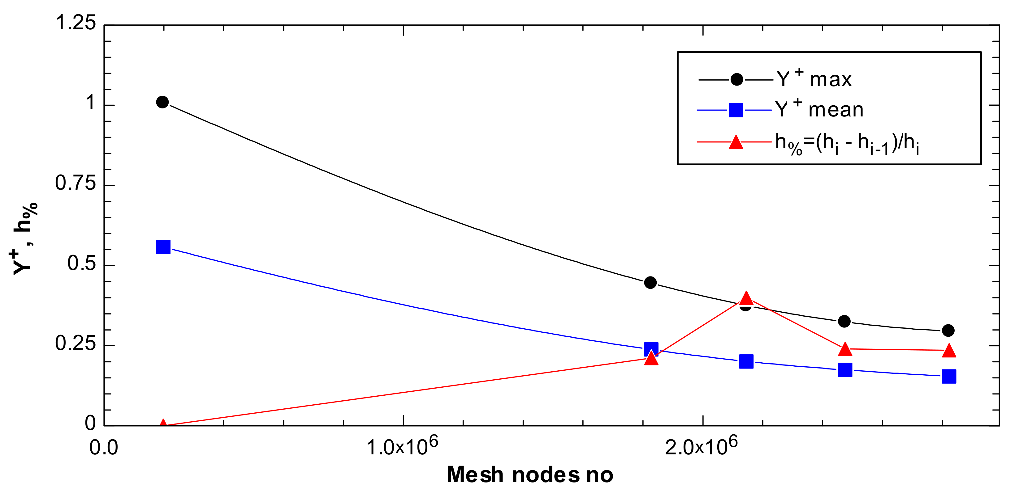
2.3. Computational Grid
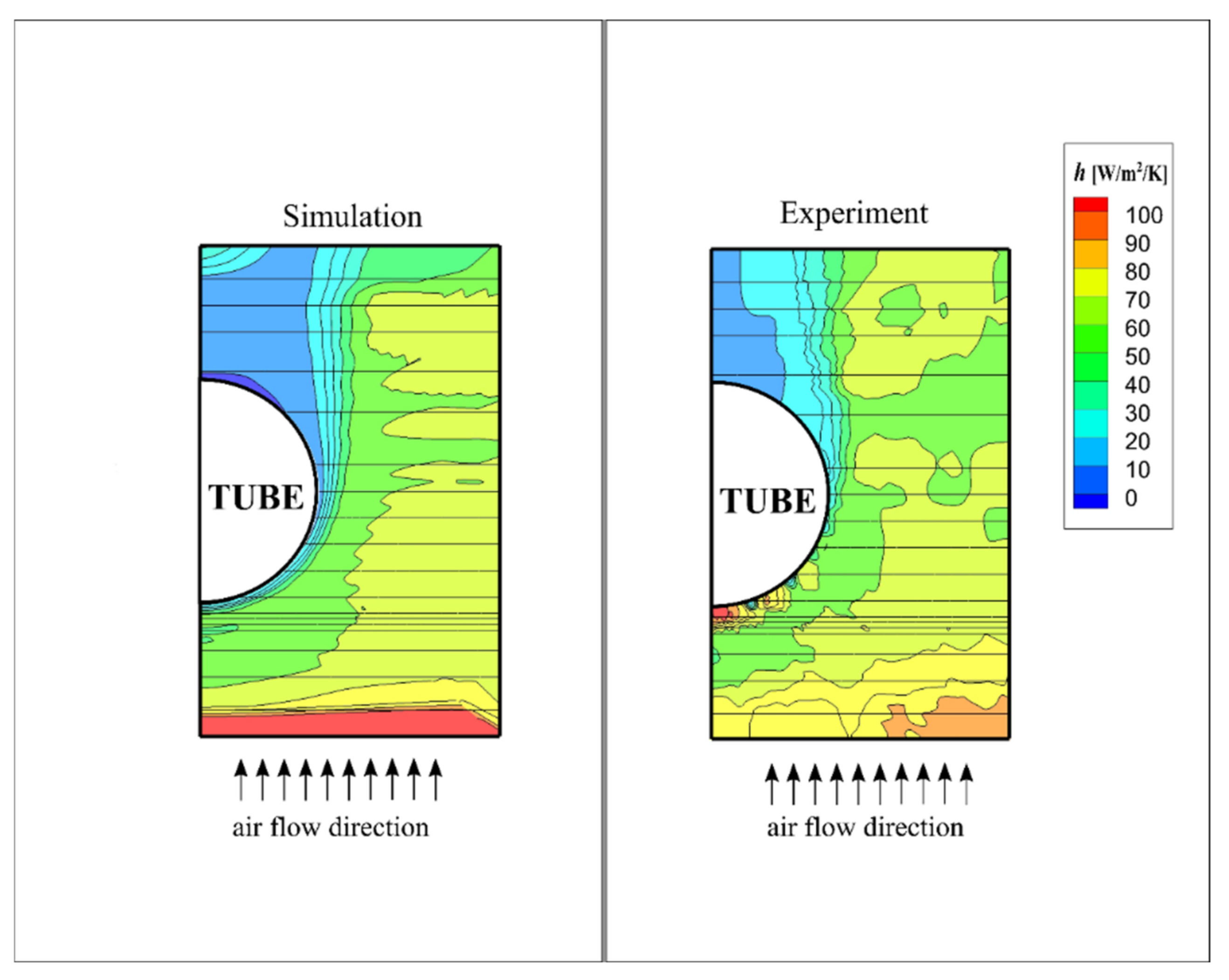
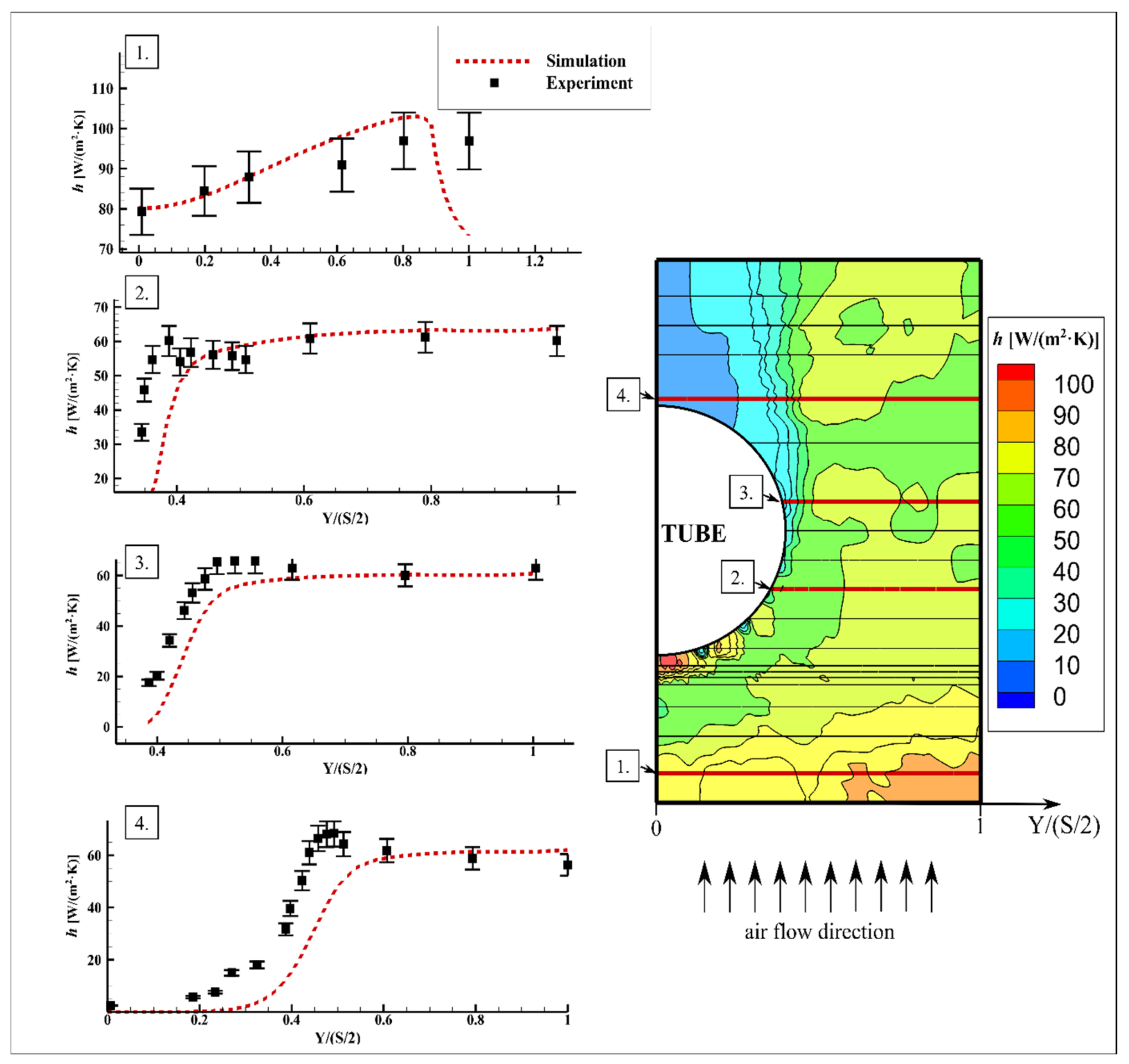
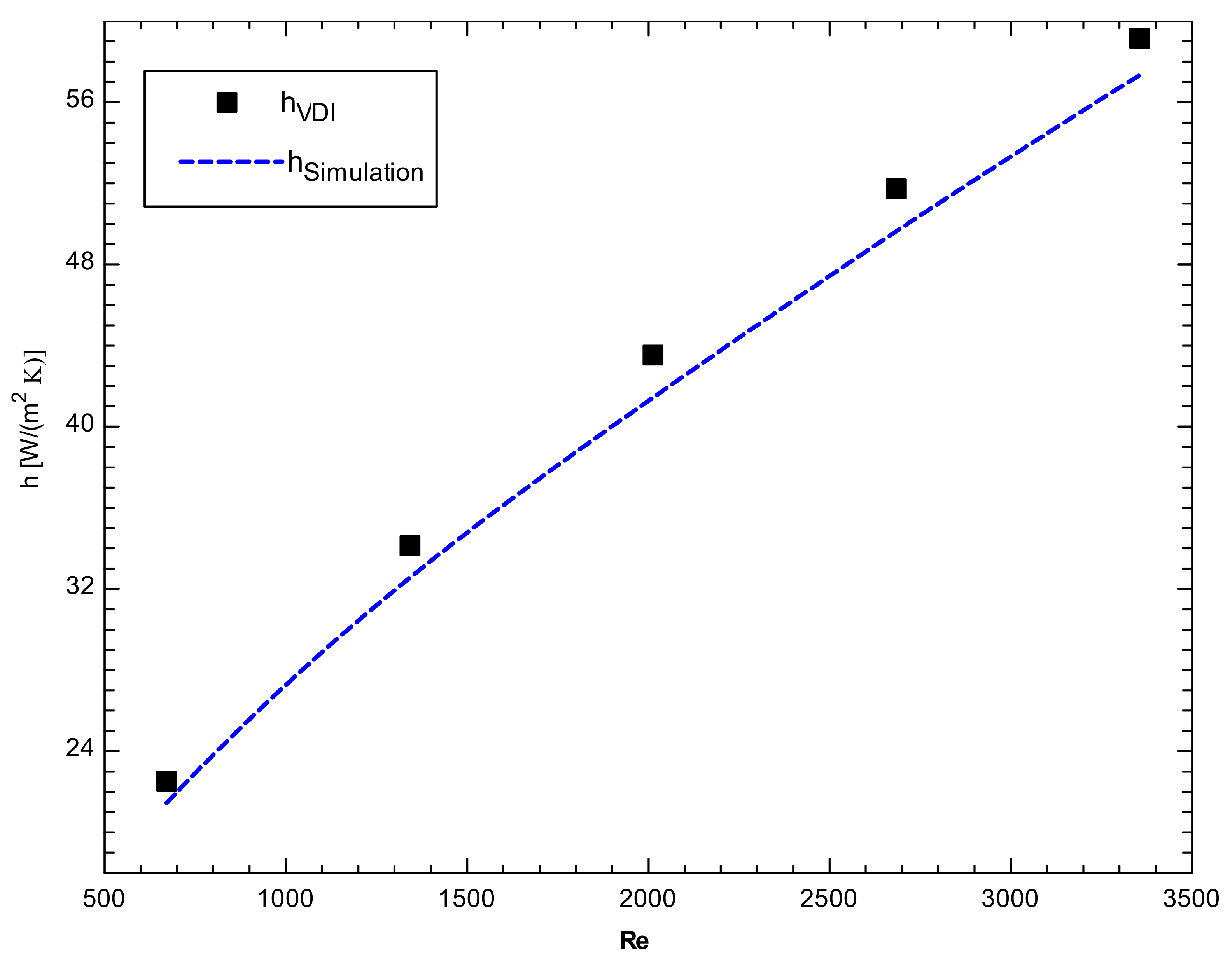
2.4. Validation of the Numerical Model
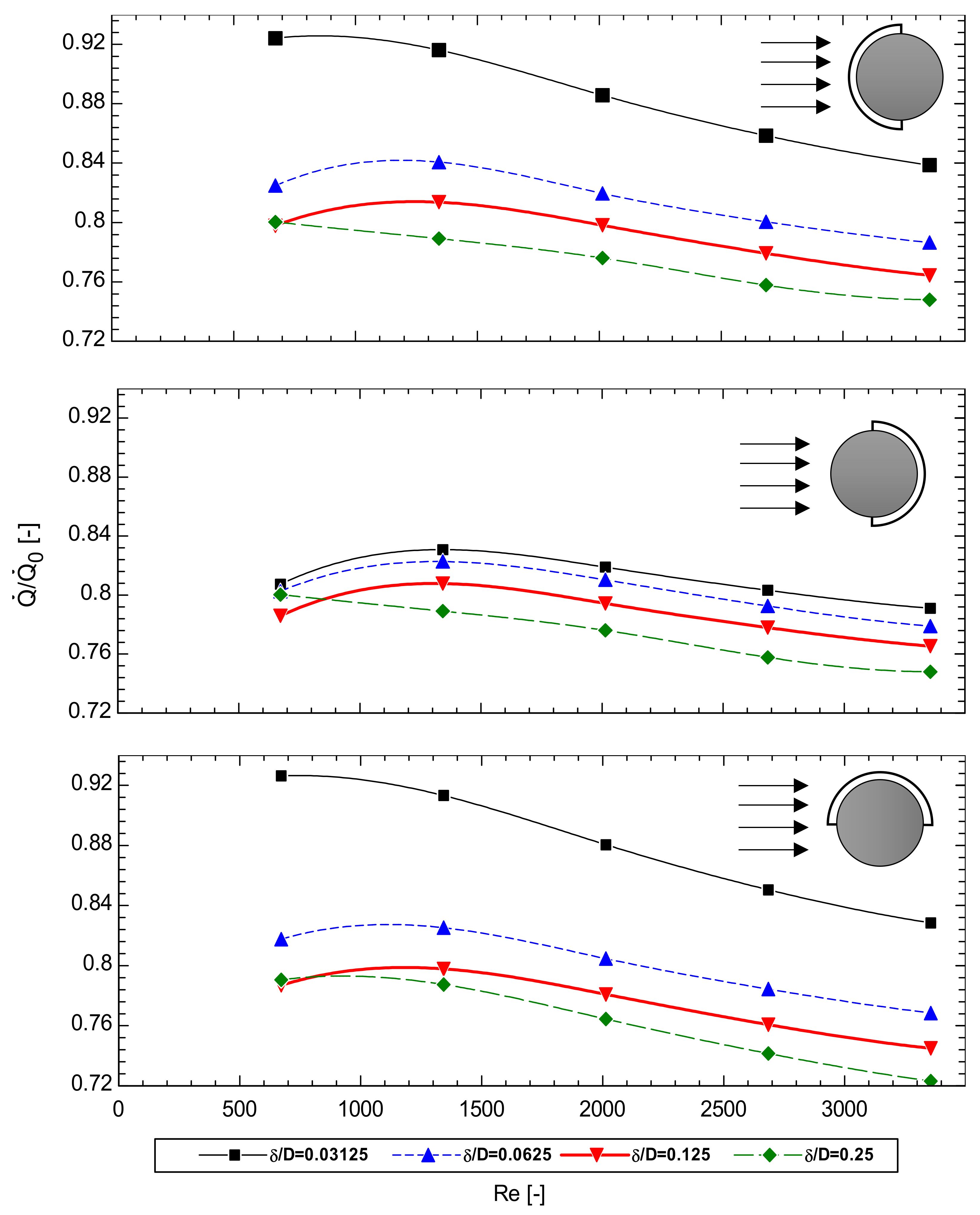
3. Results and Discussion
4. Conclusions
Author Contributions
Funding
Data Availability Statement
Conflicts of Interest
Nomenclature
| A | finned side heat transfer surface, m2 |
| At0 | bare outside tube surface, m2 |
| CFD | computational fluid dynamics |
| cp | specific heat at constant pressure, J/kg/K |
| d | diameter, m |
| dh | (4·(Lf − D)·Lt·Lf )/(2 [Lf2 − (π·D2/4)] + π·D·Lt)—hydraulic diameter, m |
| D | outer diameter of the tube |
| e | total fluid energy, J/kg |
| g | gravitational acceleration, m/s2 |
| h | heat transfer coefficient, W/m2/K |
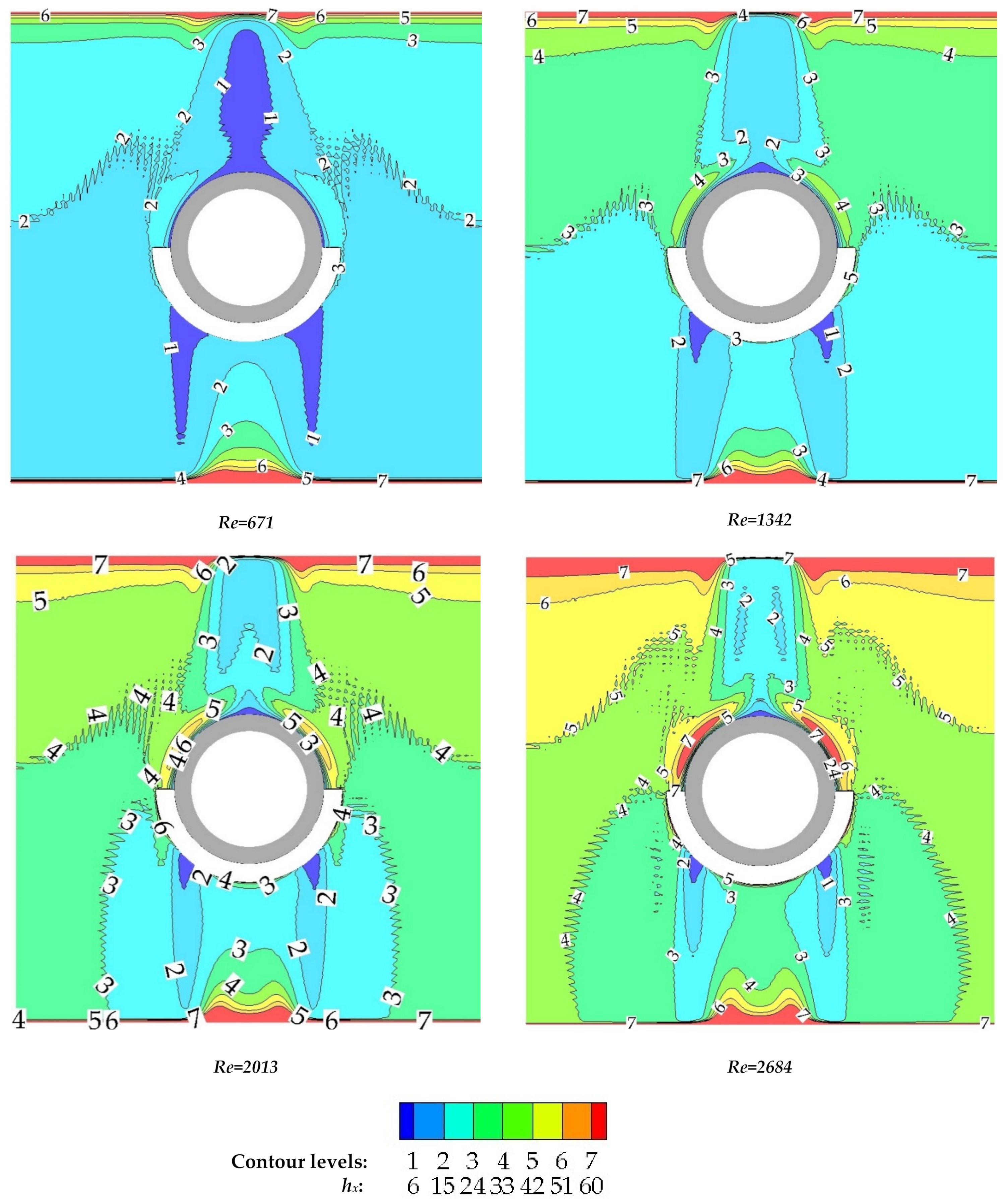
| hx | local heat transfer coefficient |
| h% | (hi − hi−1)/hi, relative change of heat transfer coefficient, % |
| k | 0.5·ui’·ui’—kinetic energy of turbulence m2/s2 |
| L | length, m |
| periodic length vector, m | |
| mass flow, kg/s | |
| n | heat-mass transfer analogy exponent |
| vector normal to a surface | |
| Nu | Nusselt number |
| p | pressure, Pa |
| periodic pressure, Pa | |
| Pr | Prandtl number |
| Prt | turbulent Prandtl number |
| heat flux (vector), W/m2 | |
| heat transfer rate, W | |
| position vector, m | |
| Re | V·dh/ν—Reynolds number |
| Ri | (g·β·ΔT·L)/V2—Richardson number |
| Sc | Schmidt number |
| Sh | Sherwood number |
| SST | shear stress transport |
| T | temperature, K |
| periodic temperature, K | |
| V | average velocity (scalar), m/s |
| u | velocity vector, m/s |
| time-averaged velocity vector, m/s | |
| x | cartesian coordinates vector, m |
| Xt | tube spacing, m |
| Y+ | non-dimensional distance between the first mesh node and the wall |
| Greek symbols | |
| β | volumetric expansion coefficient, 1/K |
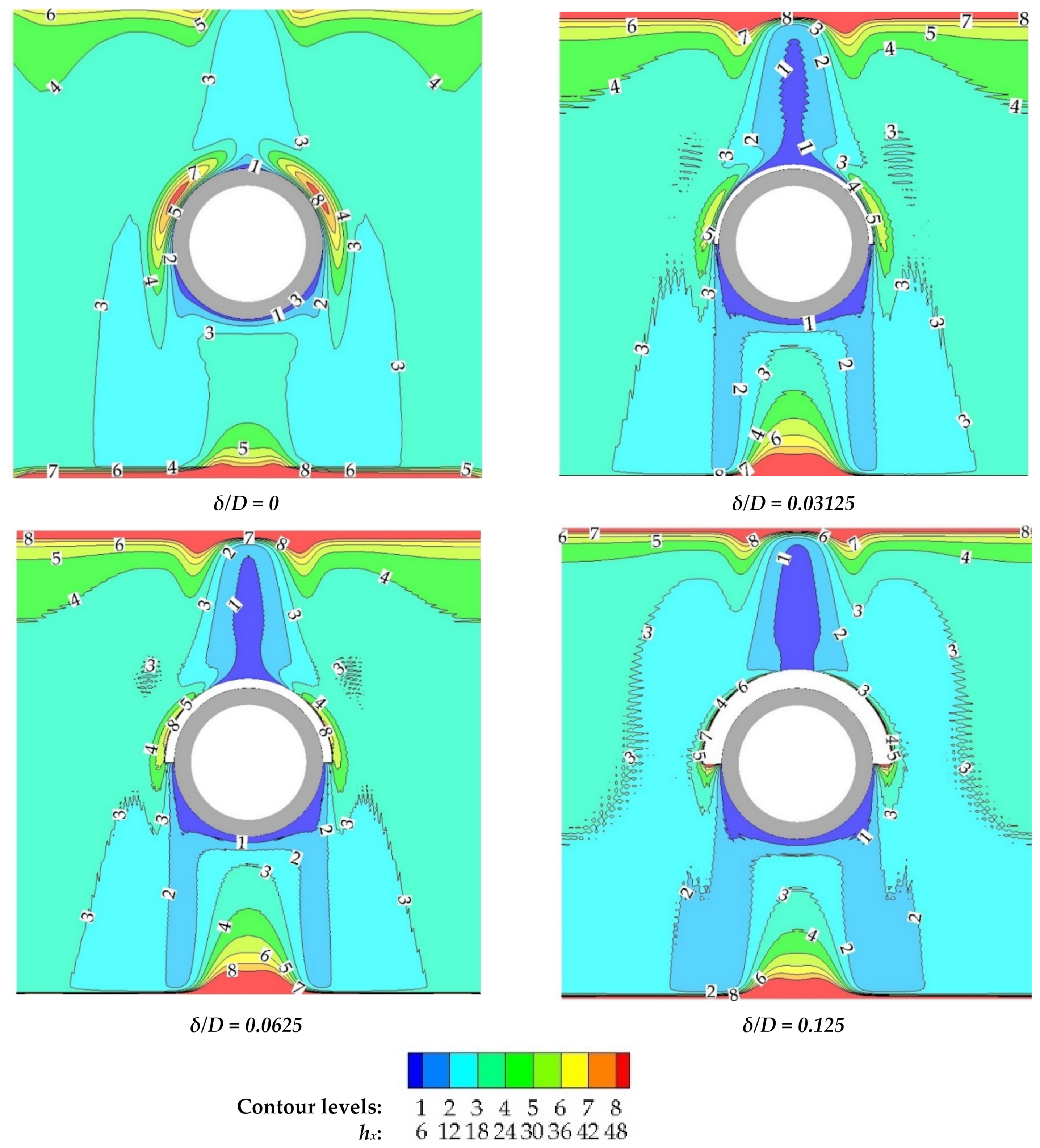
| δ | gape thickness, thickness, spacing, m |
| δij | Kronecker delta |
| Δ | difference of a quantity |
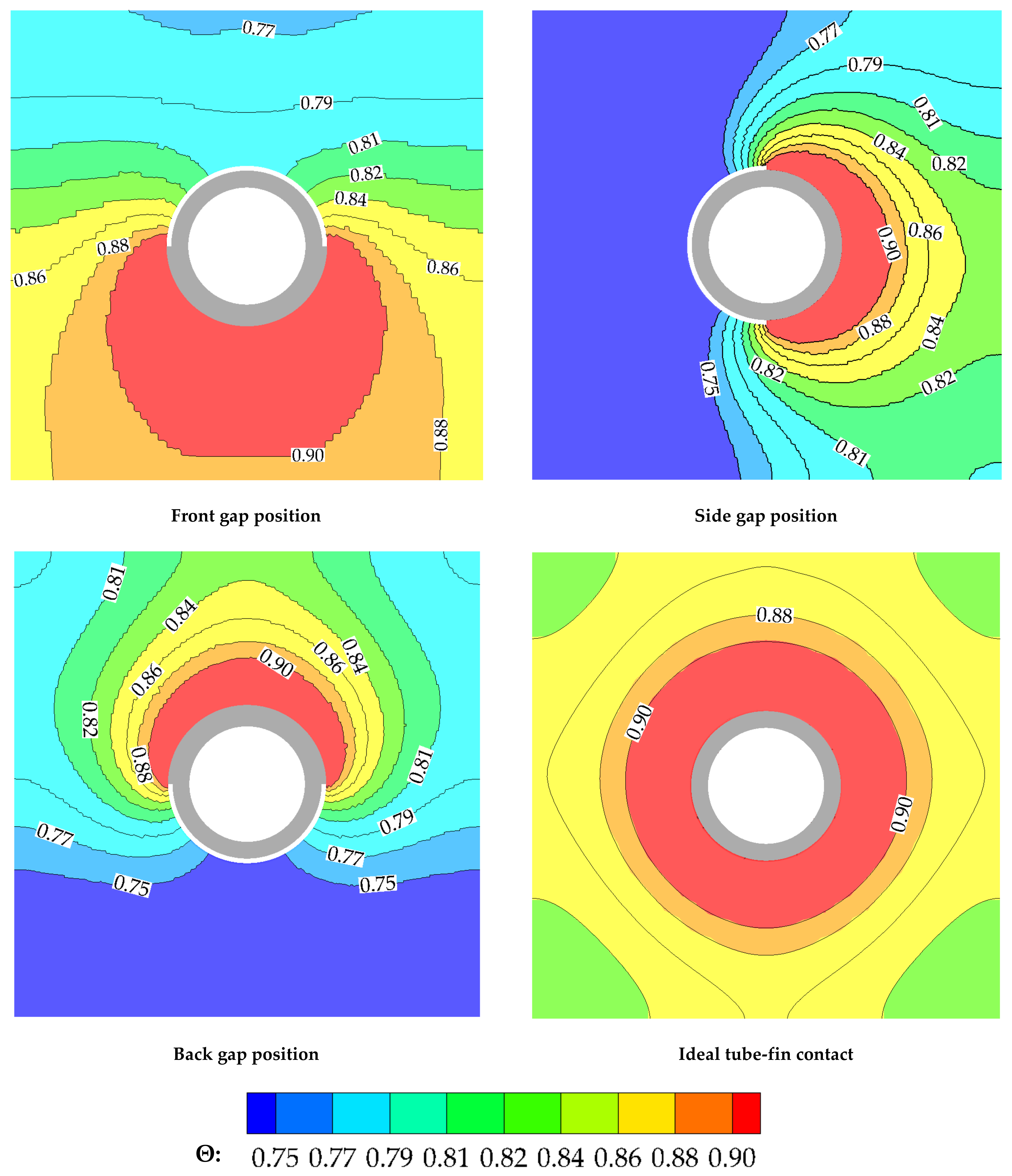
| θ | the gap placement angle |
| Θ | temperature excess |
| λ | thermal conductivity, W/m/K |
| μ | dynamic viscosity, kg·m/s |
| ν | kinematic viscosity, m2/s |
| ρ | density, kg/m3 |
| Reynolds stresses, Pa | |
| σ | linear temperature gradient, K/m |
| τij | stress tensor, Pa/m |
| ω | specific dissipation rate, 1/s |
| Subscripts | |
| 0 | zero gap thickness |
| ave | average |
| d | based on the tube outside diameter |
| f | fin |
| g | gap |
| i | inside, inner, for i-th mesh refinement |
| i, j, k | indices (1, 2, 3) |
| in | inlet |
| o | outlet, outer |
| t | tube, turbulent |
| w | wall |
References
- Gorecki, G. Investigation of two-phase thermosyphon performance filled with modern HFC refrigerants. Heat Mass Transf. 2018, 54, 2131–2143. [Google Scholar] [CrossRef] [Green Version]
- Chai, L.; Tassou, S. A Review of Airside Heat Transfer Augmentation with Vortex Generators on Heat Transfer Surface. Energies 2018, 11, 2737. [Google Scholar] [CrossRef] [Green Version]
- Taler, D.; Taler, J.; Trojan, M. Experimental Verification of an Analytical Mathematical Model of a Round or Oval Tube Two-Row Car Radiator. Energies 2020, 13, 3399. [Google Scholar] [CrossRef]
- Lotfi, B.; Sundén, B.; Wang, Q. An investigation of the thermo-hydraulic performance of the smooth wavy fin-and-elliptical tube heat exchangers utilizing new type vortex generators. Appl. Energy 2016, 162, 1282–1302. [Google Scholar] [CrossRef]
- Välikangas, T.; Karvinen, R. Conjugated Heat Transfer Simulation of a Fin-and-Tube Heat Exchanger. Heat Transf. Eng. 2018, 39, 1192–1200. [Google Scholar] [CrossRef]
- Bansal, P.; Wich, T.; Browne, M. Optimisation of egg-crate type evaporators in domestic refrigerators. Appl. Therm. Eng. 2001, 21, 751–770. [Google Scholar] [CrossRef]
- Blygold Blygold—Example of Galvanic Corrosion Damage. Available online: https://www.blygold.com/services/coil-coating/ (accessed on 15 May 2021).
- Critoph, R.; Holland, M.; Turner, L. Contact resistance in air-cooled plate fin-tube air-conditioning condensers. Int. J. Refrig. 1996, 19, 400–406. [Google Scholar] [CrossRef]
- Jannick, P.; Meurer, C.; Swidersky, H. Potential of Brazed Finned Tube Heat Exchangers in Comparison to Mechanical Produced Finned Tube Heat Exchangers. In Proceedings of the International Refrigeration and Air Conditioning Conference, West Lafayette, IN, USA, 16–19 July 2002. [Google Scholar]
- Zhao, H.; Salazar, A.J.; Sekulic, D.P. Analysis of Fin-Tube Joints in a Compact Heat Exchanger. Heat Transf. Eng. 2009, 30, 931–940. [Google Scholar] [CrossRef]
- Jeong, J.; Nyung Kim, C.; Youn, B.; Saeng Kim, Y. A study on the correlation between the thermal contact conductance and effective factors in fin–tube heat exchangers with 9.52 mm tube. Int. J. Heat Fluid Flow 2004, 25, 1006–1014. [Google Scholar] [CrossRef]
- Cheng, W.; Madhusudana, C. Effect of electroplating on the thermal conductance of fin–tube interface. Appl. Therm. Eng. 2006, 26, 2119–2131. [Google Scholar] [CrossRef]
- Taler, D.; Ocłoń, P. Thermal contact resistance in plate fin-and-tube heat exchangers, determined by experimental data and CFD simulations. Int. J. Therm. Sci. 2014, 84, 309–322. [Google Scholar] [CrossRef]
- Taler, D.; Cebula, A. A new method for determination of thermal contact resistance of a fin-to-tube attachment in plate fin-and-tube heat exchangers. Chem. Process Eng. 2010, 31, 839–855. [Google Scholar]
- Singh, S.; Sørensen, K.; Condra, T.J. Influence of the degree of thermal contact in fin and tube heat exchanger: A numerical analysis. Appl. Therm. Eng. 2016, 107, 612–624. [Google Scholar] [CrossRef]
- Saboya, F.E.M.; Sparrow, E.M. Local and Average Transfer Coefficients for One-Row Plate Fin and Tube Heat Exchanger Configurations. J. Heat Transf. 1974, 96, 265. [Google Scholar] [CrossRef]
- Menter, R.F. Zonal Two Equation Kappa-Omega Turbulence Models for Aerodynamic Flows. In Proceedings of the 23rd Fluid Dynamics, Plasmadynamics, and Lasers Conference, Orlando, FL, USA, 6–9 July 1993. [Google Scholar]
- Lindqvist, K.; Skaugen, G.; Meyer, O.H.H. Plate fin-and-tube heat exchanger computational fluid dynamics model. Appl. Therm. Eng. 2021, 189, 116669. [Google Scholar] [CrossRef]
- Taler, D.; Ocłoń, P. Determination of heat transfer formulas for gas flow in fin-and-tube heat exchanger with oval tubes using CFD simulations. Chem. Eng. Process. Process Intensif. 2014, 83, 1–11. [Google Scholar] [CrossRef]
- Jasiński, P.B. Numerical study of the thermo-hydraulic characteristics in a circular tube with ball turbulators. Part 2: Heat transfer. Int. J. Heat Mass Transf. 2014, 74, 473–483. [Google Scholar] [CrossRef]
- Ocłoń, P.; Łopata, S. Study of the Effect of Fin-and-Tube Heat Exchanger Fouling on its Structural Performance. Heat Transf. Eng. 2018, 39, 1139–1155. [Google Scholar] [CrossRef]
- Ansys Inc. ANSYS CFX Theory Guide; Ansys Inc.: Canonsburg, PA, USA, 2013. [Google Scholar]
- Shevchuk, I.V.; Jenkins, S.C.; Weigand, B.; Von Wolfersdorf, J.; Neumann, S.O.; Schnieder, M. Validation and analysis of numerical results for a varying aspect ratio two-pass internal cooling channel. J. Heat Transf. 2011, 133. [Google Scholar] [CrossRef]
- Siddique, W.; El-Gabry, L.; Shevchuk, I.V.; Fransson, T.H. Validation and Analysis of Numerical Results for a Two-Pass Trapezoidal Channel With Different Cooling Configurations of Trailing Edge. J. Turbomach. 2012, 135. [Google Scholar] [CrossRef] [Green Version]
- Goldstein, R.J.; Cho, H.H. A review of mass (heat) transfer measurements using naphthalene sublimation. Exp. Heat Transf. Fluid Mech. Thermodyn. 1993, 10, 21–40. [Google Scholar] [CrossRef]
- Kays, W.M.; William, M.; London, A.L.; Alexander, L. Compact Heat Exchangers; Krieger Pub. Co.: Malabar, FL, USA, 1998; ISBN 1575240602. [Google Scholar]
- Rosman, E.C.; Carajilescov, P.; Saboya, F.E.M. Performance of One- and Two-Row Tube and Plate Fin Heat Exchangers. J. Heat Transf. 1984, 106, 627. [Google Scholar] [CrossRef]
- Tecplot Inc. Tecplot.360 EX User’s Manual; Tecplot Inc.: Bellevue, WA, USA, 2018. [Google Scholar]
- Saboya, S.M.; Saboya, F.E.M. Transfer coefficients for plate fin and elliptical tube heat exchangers. In Proceedings of the 6th Brazilian Congress of Mechanical Engineering, Rio de Janeiro, Brazil, 15–18 December 1981. [Google Scholar]
- Stephan, P. B1 Fundamentals of Heat Transfer. In VDI Heat Atlas; Springer: Berlin/Heidelberg, Germany, 2010; pp. 15–30. [Google Scholar]


| Description | Symbol | Value [mm] |
|---|---|---|
| Length and width of the fin | Lf | 25 |
| Tube length | Lt | 2.5 |
| Outside diameter of the tube | D | 8 |
| Internal diameter of the tube | di | 6.2 |
| Fin thickness | δf | 0.05 |
| Gap thickness | δ | 0.25–2.0 |
| Tube spacing | Xt | 12.5 |
Publisher’s Note: MDPI stays neutral with regard to jurisdictional claims in published maps and institutional affiliations. |
© 2021 by the authors. Licensee MDPI, Basel, Switzerland. This article is an open access article distributed under the terms and conditions of the Creative Commons Attribution (CC BY) license (https://creativecommons.org/licenses/by/4.0/).
Share and Cite
Łęcki, M.; Andrzejewski, D.; Gutkowski, A.N.; Górecki, G. Study of the Influence of the Lack of Contact in Plate and Fin and Tube Heat Exchanger on Heat Transfer Efficiency under Periodic Flow Conditions. Energies 2021, 14, 3779. https://doi.org/10.3390/en14133779
Łęcki M, Andrzejewski D, Gutkowski AN, Górecki G. Study of the Influence of the Lack of Contact in Plate and Fin and Tube Heat Exchanger on Heat Transfer Efficiency under Periodic Flow Conditions. Energies. 2021; 14(13):3779. https://doi.org/10.3390/en14133779
Chicago/Turabian StyleŁęcki, Marcin, Dariusz Andrzejewski, Artur N. Gutkowski, and Grzegorz Górecki. 2021. "Study of the Influence of the Lack of Contact in Plate and Fin and Tube Heat Exchanger on Heat Transfer Efficiency under Periodic Flow Conditions" Energies 14, no. 13: 3779. https://doi.org/10.3390/en14133779