Energy Fluctuations in the Homogenized Hyper-Elastic Particulate Composites with Stochastic Interface Defects


Department of Structural Mechanics, Lodz University of Technology, 90-924 Łódź, Poland
*
Author to whom correspondence should be addressed.
Energies 2020, 13(8), 2011; https://doi.org/10.3390/en13082011
Submission received: 16 March 2020
/
Revised: 11 April 2020
/
Accepted: 14 April 2020
/
Published: 17 April 2020
(This article belongs to the Special Issue Recent Advances in Stochastic Methods for Energy Analysis)
Abstract
:The principle aim of this study is to analyze deformation energy of hyper-elastic particulate composites, which is the basis for their further probabilistic homogenization. These composites have some uncertain interface defects, which are modelled as small semi-spheres with random radius and with bases positioned on the particle-matrix interface. These defects are smeared into thin layer of the interphase surrounding the reinforcing particle introduced as the third component of this composite. Matrix properties are determined from the experimental tests of Laripur LPR 5020 High Density Polyurethane (HDPU). It is strengthened with the Carbon Black particles of spherical shape. The Arruda–Boyce potential has been selected for numerical experiments as fitting the best stress-strain curves for the matrix behavior. A homogenization procedure is numerically implemented using the cubic Representative Volume Element (RVE). Spherical particle is located centrally, and computations of deformation energy probabilistic characteristics are carried out using the Iterative Stochastic Finite Element Method (ISFEM). This ISFEM is implemented in the algebra system MAPLE 2019 as dual approach based upon the stochastic perturbation method and, independently, upon a classical Monte-Carlo simulation, and uniform uniaxial deformations of this RVE are determined in the system ABAQUS and its 20-noded solid hexahedral finite elements. Computational experiments include initial deterministic numerical error analysis and the basic probabilistic characteristics, i.e., expectations, deviations, skewness and kurtosis of the deformation energy. They are performed for various expected values of the defects volume fraction. We analyze numerically (1) if randomness of homogenized deformation energy can correspond to the normal distribution, (2) how variability of the interface defects volume fraction affects the deterministic and stochastic characteristics of composite deformation energy and (3) whether the stochastic perturbation method is efficient in deformation energy computations (and in FEM analysis) of hyper-elastic media.
1. Introduction
Interface defects are the very important engineering problem in composite materials. This is because they are the result of many manufacturing processes, they remarkably affect their mechanical (and coupled) response and occupy relatively small total volume fraction of the entire composite. They affect failure [1,2], reliability [3], durability [4] and thermal conductivity [5] of the composite and can be included in numerical analysis as geometrical imperfections [6]. Alternatively, interface defects can be represented as imperfect interfaces, which commonly serve for a realistic prediction of composites behavior [7,8]. They can also be adjusted to fine tune the characteristics of composites for specific needs [1,9]. Defective composites are investigated with an additional thin layer between its initial constituents [8,10,11,12,13] defined as the interphase. This model follows some manufacturing processes relevant to the polymeric composites where glassy phases may occur around the reinforcing fibers of particles due to thermal processing of such a composite. A very similar interphase can be noticed in rubber-based mixtures, where the occluded rubber forms some kind of the thin interphase about the reinforcing carbon particles. Other numerical approaches to the interface defects include introduction of a system of springs [14] or addition of specific contact finite elements [15]. As it has been documented, this interphase is the weakest link in composite structures and significantly affects effective (homogenized) material properties of multiple composites irrespective to their degree of anisotropy and also outside of the deterministic context. They affect probabilistic and stochastic characteristics of these composites [16,17]. An increase of probabilistic dispersion of defects volume fraction results in a considerable uncertainty in mechanical properties of entire composite and an increase of their amount typically causes degradation of these properties. An influence of the interphase could be either negative, in the case when the bond between the main constituents is weak or defective [18], or positive in the presence of chemical bonds between the principal phases [19,20], for example in bound rubber. Early approach to homogenization of composites included a pure analytical apparatus. It was strictly limited in application to linear elastic, reversible and isotropic constituents and also required a simple pattern of periodicity of the Representative Volume Element (RVE) [21,22,23]. Contemporary studies use a multi-scale approach rather to represent a nonlinear response for composites, elasto-plastic, visco-elasto-plastic and also the hyper-elastic one [24,25,26,27]. In such studies, deformation energy is necessary for determination of nonlinear model parameters but only few of them [27,28] focus on it directly. Nevertheless, they do not address the fundamental question of how the interface defects affect deformation process uncertainty of the composite and are not based on experimental tests for a specific material, which is done in this study.
The principle aim of this work is to determine how the initial stochastic interface defects affect the deformation process of a composite under classical uniaxial tension experiment; a dual probabilistic approach to the hyper-elastic problem is proposed here to achieve this goal. This is done to validate the Iterative Stochastic Finite Element Method (ISFEM)computation against the classical Monte-Carlo simulation [29] and provide an efficient alternative offering a reduced computational time and requiring less computer resources. The ISFEM is based on the iterative stochastic perturbation approach and is augmented with a supplementary FEM implementation. The deformation energy is determined with use of the homogenization technique and computed with the Finite Element Method (FEM) based on displacements. A unitary cubic Representative Volume Element (RVE) is used. The matrix of this composite is applied after laboratory tests of Laripur LPR 5020 and the particles are modeled as Carbon Black Fullerenes F60.
Stochastic perturbation approach is based on a cyclic FEM usage with a fluctuating parameter for numerical recovery of the polynomial response function relating the resulting deformation energy with the given uncertain initial parameter, i.e., interface defects volume fraction. The input parameter is included in a polynomial form directly in the effective strain energy of the composite that is based on Arruda–Boyce potential or, alternatively, this relation is represented as a bivariate polynomial. It is used for calculation of the first four probabilistic characteristics of the structural response using stochastic perturbation approach based upon the general order Taylor expansion.
2. Methods
Let us introduce a continuous and heterogeneous solid body in 3D Euclidean space Ω visualized on Figure 1. It describes a particle-reinforced composite and contains three distinct phases—matrix , interphase and particles and so that
The matrix and an interphase are both hyper-elastic and particles linear elastic. It is further assumed that a contact in-between matrix and interphase as well as in-between the particle and the interphase too is perfect and also load-independent. Further, it is mandatory to assume that interphase and the particle does not intersect the outer surfaces of the RVE , so that .
Total defects volume in the given RVE can be expressed via summation of all the defects contributions as follows
A single interface defect is approximated with semi-spherical shape penetrating the matrix and a geometrical center of such a defect is each time located on the particle surface. Each defect radius R is assumed to be statistically dispersed according to the normal distribution and is defined by its expected value E[R] and variance Var(R). Next, such a defected interface is replaced with the interphase (as artificial layer around the particle) having constant thickness around the particle, which includes all the interface defects and small portions of the matrix surrounding them. This thickness also serves as the upper limit of the defects radii that is limited by a three sigma rule
where is a thickness of hyper-elastic interphase which surrounds a particle. All material characteristics of the interphase necessary for further numerical simulation are simply calculated as volumetric average of the matrix and the defects contributions. Similarly, the effective stress of the interphase is recovered using the rule of mixtures connected to volumetric contributions of the matrix and the defects contained in
where denotes the stress intensity in the matrix contained in the interphase and stress intensity in the defects. The first two probabilistic moments of σint are further represented as
Let us next assume that defects do not provide a contribution for the stress and introduce a parameter denoting their volume fraction, so that
and let us assume that this parameter is independent of the strain level. Its characteristics, i.e., expectation and variance are determined analytically from E[R] and Var(R) using the basic definitions of probability theory; some details may be found in Appendix of the reference [16]. Multi-scale homogenization scheme is proposed to model their impact on the composite in its macro-scale and it consists of three steps. Firstly, the interphase is replaced with the new artificial material surrounding all the particles. Secondly, the interface defects are probabilistically averaged throughout the corresponding interphases. Finally, the composite is probabilistically homogenized together with all these interphases. A micro-geometry of this composite has been schematically given in Figure 2. Deformation gradient of hyper-elastic matrix is defined as , where represents the spatial configuration and describes the reference configuration and deformation energy accumulated in the matrix can be described as
where is the right Cauchy-Green deformation tensor.
Let us assume that this matrix is incompressible, its behavior depends upon the first two invariants only and that it can be efficiently represented by the Arruda–Boyce model [30]. Then, its energy can be calculated as
where is an additional material parameter, , stands here for the locking stretch of the polymer chain networks, while define the additional coefficients (given in Table 1). The effective strain energy of homogenized composite depends on the invariants and interface defects volume fraction. It could further be divided into three independent contributions—of the matrix, of the interphase and of the particle, independently. There holds
Consecutively, we rewrite a deformation energy formula adjacent to the Arruda–Boyce model using parameters corresponding to the homogenized composite , which additionally depend upon the interface defects volume fraction so that
It is aimed for composites with much softer matrix than the reinforcement. In such composites, deformation of stiff reinforcement is very small so that and the major contribution to deformation energy comes from hyper-elastic components. The relation between the stiffness tensor and the weakening coefficient is determined with two steps (a) material coefficients are calculated on the basis of the FEM experiments solved sequentially with varying and (b) these coefficients are replaced by a continuous polynomial with respect to proposed as
This polynomial is optimized with use of the Least Squares by maximization of correlation between the lab results and the computations as well as minimization of variance and error of the LSM. Such an approximation ensures continuous relation to and and introduces a very small error. The second formulation is based on the following approximation of the strain energy as a bivariate polynomial so that
where polynomial coefficients are denoted by and its rank by n. This approximation is next optimized in a two-step procedure. Firstly, a regression is applied for determination of polynomial coefficients with ranks between 1 and 12. Secondly, the optimum rank is selected that ensures a minimum LSM error. However, the principle objective of this study is to analyze numerically the deformation energy U for the hyper-elastic composite. Let denote the position vector related to the non-deformed body configuration, position vector related to the deformed configuration and displacement vector. Let us define in the three-dimensional physical space for the given material the Green–Lagrange strain tensor as
Let us define introduce the second Piola–Kirchhoff stress tensor as
where is the Jacobian of transformation from non-deformed to a deformed coordinate system. By definition of the hyper-elastic material we have the following relation:
where is an elastic potential dependent on the invariants of the strain tensor. One can derive the general constitutive relation for hyper-elastic isotropic material from the formula (15) as [30]
where is a derivative of the elastic potential with respect to the i-th invariant of the strain tensor
Finally, we calculate elastic strain energy in a traditional way as
It is done by assuming various forms of the elastic potential W corresponding to the constitutive models of hyper-elastic materials contrasted in numerical analysis and summarized in the table below. As it is seen, Arruda–Boyce theory adopted to the stochastic interface theory, includes higher powers of the strain tensor first invariant. So that, a precise initial FEM error analysis is extremely important to avoid any computational discrepancies during deformation energy determination; one could consider an application of some mesh adaptation procedure.
The Finite Element Method discretization of the entire RVE has been prepared with the use of 20-node three-dimensional iso-parametric finite element in three-dimensional physical space called C3D20 in ABAQUS. Let us introduce the global coordinate system and the local normalized coordinate system . The global coordinates of the i-th node after deformation we denote as respectively.
where are the applied shape functions:
- -
- for corner nodes:
- -
- for side nodes:
The coordinates of the element nodes in the local system are shown in Figure 3.
We consider an iso-parametric finite element, so we can use the same shape function functions (20) to describe displacements increments
where Δq is a vector containing the increments of the given degrees of freedom. Equation (24) can be further used to discretize the strain tensor increments Δε defined previously in formula (13) and one arrives at
The matrix B includes all spatial derivatives of the shape functions N. This allows for a determination of the stress tensor increments in the following way:
where is strain-dependent constitutive tensor. A parametrization of this FEM model with respect to the interphase parameter w necessary in further Stochastic Finite Element Method implementation proceeds by a selection of the set of real values of this parameter taken from a certain neighborhood of its mean value, sequential recalculation of several FEM models with varying w and the Least Squares Method approximation of approximating polynomials independently for strains, stresses and energies (similarly to the formula (11)). Final calculation of the stochastic moments of the energy follows the classical integral definition of the kth central probabilistic moment, which is
The right hand side is expanded using random Taylor series of the following form:
where is the mean value of effective energy under consideration, which means effective energy calculated for the mean value of the parameter w, and where odd order terms simply vanish. Such a procedure for the first four probabilistic moments of energy and for the given polynomial basis has been entirely programmed in MAPLE 2019, whose results are presented below.
3. Results and Discussion
3.1. Deterministic Numerical Experiments
Numerical experiments are done according to the homogenization method with use of a hexagonal Representative Volume Element (RVE). This RVE has unit dimensions and consists of three phases, i.e., the polymeric matrix that occupies 90% of the RVE volume, as well as a spherical particle and the surrounding interphase, that occupy remaining 10% of the RVE, 5% each. Linear elastic particles of carbon black have initial mechanical properties equal to and . The matrix and the interphase are modeled after the laboratory tests of Laripur LPR 5020. Fitting is provided with the Arruda–Boyce hyper-elastic potential and a set of parameters of chosen from 10 different hyper-elastic models because it ensured optimal fitting to laboratory data. A surface-based tie constraint is selected for modeling a perfectly rigid contact. The interface defects volumetric ratio takes the value 0, when interphase is perfect and 1, when this interphase is composed from the defects only. Deformation energy of uniaxial stretch is computed with an implicit solver available in the FEM system ABAQUS. It is recovered from a series of cell problems, in which particle has been discretized using the hexahedral 20-noded C3D20 finite elements and the remaining phases—with the hybrid linear pressure C3D20H finite elements; the entire mesh shown in Figure 4 consists of about 150,000 finite elements. The full Newton algorithm has been applied in incremental analysis and the direct sparse multi-front equation solver has been used. The displacement of outer edges of the RVE is linearly increased in each increment of analysis. Size of increments ranges between and , while the outputs are recovered exactly 55 times during the deformation process for for each FEM realization. The model of the matrix is optimized to best represent the mean value of the uniaxial tension laboratory tests of 10 specimens. The model used in further study is chosen by minimization of the total LSM error among 10 different hyper-elastic potentials. The fitting of material parameters is done by the Least Squares Method (LSM) with equal weights.
Fittings and results of laboratory tests (marked by the green points) are presented in Figure 5. They include 10 different potentials, namely the reduced (2nd order) and full polynomials (2nd, 4th, 5th and 6th order) as well as Neo–Hookean [31,32], Arruda–Boyce [33], Yeoh [34] and Mooney–Rivlin [35,36] models. Arruda–Boyce potential has been selected for further analysis with the following parameters: . It overestimates a little bit an overall value of the longitudinal stress at the strain level close to , but ensures at the same time an efficient overall estimation. As the confirmation one may notice that maximum stress coming from laboratory tests equals to and the one calculated from the Arruda–Boyce is equal to ; two other potentials ensuring relatively good fitting are the Mooney–Rivlin and the Neo–Hookean potentials.
Figure 6 reports a fluctuation of the effective deformation energy w.r.t. the interface defects volume fraction and for an increasing level of strain . The direct output of the FEM simulations is marked as ‘FEM’, the functional approximation as ‘LSM’ and a bivariate polynomial approximation as ‘BPO’ on this figure. It illustrates that the deformation energy exponentially increases together with an additional increase of the strain level and it has a converse relation with for all levels of the strain. Effective deformation energy differs approximately by 40% between and for the highest considered strain level and this decrease gets smaller together with decrease of .
Further, a relative error of the LSM and BPO is illustrated in Figure 7, which has been calculated as follows
Thanks to the series of previous computer experiments with this composite [37], an overall numerical error has been limited to the values equal or smaller than 1%, see Figure 7. It is a little bit expected that this error variations resulting from strain level fluctuations form quite regular patterns and typically decreases together with an increase of the strain level. An influence of the interface defects is of the accidental nature, where the extreme values are obtained for the defects of the smallest size and this deserves more detailed FEM tests, possibly with multiscale direct modelling of these defects. Such an analysis could be provided using the NURBS technique implemented together with stochastic perturbation-based formulation of the FEM [38,39]. Quite analogous observation concerns a coincidence of the BPO and the FEM series—they coincide almost perfectly while varying the strain level, whereas uniform changes of the parameter w results in accidental coincidence.
3.2. Stochastic Numerical Analysis
The final study includes computation of stochastic characteristics of the composite effective deformation energy relative to statistical variability of the input random parameter . These analyses are performed thanks to the common usage of the systems ABAQUS and MAPLE 2019. They are performed for fluctuating expectation of the interface defects volume fraction in range of , for its increasing coefficient of variation and for different levels of the uniaxial strain within . Approximating optimal polynomials have 5th or 6th order, whereas some numerical studies available in the literature provide linear approximation for the same phenomenon [40]. The probabilistic characteristics analyzed in this study include the expected value (Figure 8), coefficient of random dispersion (Figure 9), skewness (Figure 10) and kurtosis (Figure 11) of the resulting ; skewness is output distribution asymmetry measure and kurtosis is output distribution concentration measure. These characteristics are determined separately with two independent methods, i.e., the fourth order iterative stochastic perturbation technique (SPT) and Monte-Carlo simulation (MCS) computed for 250,000 trials for any discrete point given in these figures. Computation is based on the full bivariate polynomial. Its coefficients are optimized with use of WLSM of equal weights and optimum rank is chosen among first ten orders. Equal weighing is preferred over Dirac weighting scheme because all the computations are based on a single bivariate polynomial and the expected value of differs among realizations. It must be highlighted that computer resources required by the perturbation-based approach are much smaller than the ones necessary for Monte-Carlo simulation and time efficiency is also significantly better; the latter method is able to provide only discrete results that are marked on subsequent graphs with an asterisk.
The expectations of the effective deformation energy presented in Figure 8 are practically independent of the input random dispersion , decrease together with an increase of expected value of defects volume fraction and increase together with an additional increase of . A limited influence of on is quite common for the Gaussian input parameters and was also recognized for the elastic case in [17]. An extent of decrease of between extreme is comparable to the deterministic case presented on Figure 6.
Coefficients of variation presented in Figure 9 are practically independent of and increase together with an increase of the coefficient of variation of an input random variable as well as its expectation. Quite importantly, for is nearly 10 times lower than for , which means that the volume fraction of defects in the composite plays a crucial role not only for the energy itself but also its dispersion; this dispersion is smaller than the one of but considerable knowing the volume fraction of defects ( means that corresponds to approx. 0.005 ). Correspondence of the two probabilistic methods for these basic probabilistic characteristics (, ) is perfect for the entire analyzed statistical scattering. This means remarkable time savings in computational analysis since a time effort of the stochastic perturbation technique is closer to a several solutions of the FEM problem than to the statistical large size repetitive solution of the homogenization problem typical for the Monte-Carlo analysis.
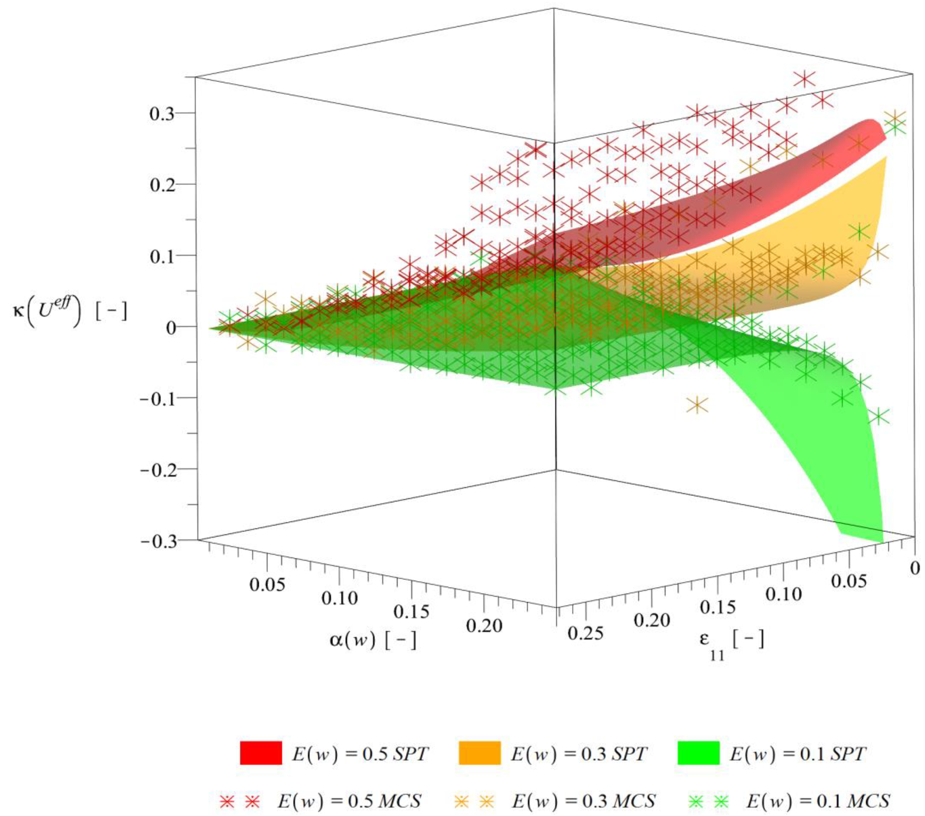
Higher order probabilistic characteristics, i.e., skewness (Figure 10) and kurtosis (Figure 11) are both increasing their magnitude together with an increase of as well as and generally decreasing in magnitude together with an increase of . Skewness remains always negative, whereas kurtosis—almost always positive. The level of the strain is important especially for low strains, for which the magnitudes of characteristics and their rate of change are the highest. Results of alternative probabilistic methods are still very good. Some differences are noticeable only for skewness with strains close to 0 and very high as well as for kurtosis with and .
The resulting homogenized deformation energy is definitely not Gaussian because of a non-zero skewness and kurtosis—its PDF changes character together with a change of the level of the strain and this result is similar to other stochastic interphase models [41]. Characteristics are most sensitive to strain changes close to zero and are also not unique for . An increase of always decreases expectation and increases dispersion as well as magnitudes of higher order characteristics. This means that interface defects are not only decreasing overall deformation energy of the composite but also increase a band of possible deformation curves. Moreover, higher order probabilistic characteristics computed using stochastic perturbation technique, even in the iterative mode [42], do not coincide with the statistical estimators of skewness and kurtosis computed via the Monte-Carlo scheme. They diverge from each other remarkably especially while increasing input coefficient of variation of the interphase parameter w.
4. Conclusions
It has been demonstrated here by numerical simulation that stochastic interface defects remarkably affect deformation process of the given composite. They considerably decrease a deformation energy of the homogenized composite at all the strain levels (up to 40%) and also cause its noticeable dispersion up to 5%. The resulting deformation energy cannot have Gaussian distribution and its PDF varies for different levels of the strain, especially close to 0. This means that application of a constant uncertain parameter independent of strain level for this composite is incorrect. The expected interface defects volume fraction has an influence on magnitudes of all stochastic characteristics of . The lower ones, i.e., expected value and coefficient of variation are increased and the higher ones, i.e., skewness and kurtosis are decreased together with its increase. The is almost independent of and all higher probabilistic characteristics of always increase their magnitude when dispersion of the defects volume fraction increases. It is verified here that the proposed defective composite model is efficient in catching the degradation of composite structural response with an increasing volume fraction of interface defects; numerical error of this FEM approximation is always kept below a single percent. Further, it is proved here that the iterative stochastic-perturbation technique implemented in conjunction with the Finite Element Method is efficient and reliable for calculation of the first four probabilistic characteristics of deformation process in hyper-elastic particle-reinforced composites with uncertain interface defects. The coincidence of the proposed stochastic perturbation-based method with statistical analysis using classical Monte-Carlo simulation is almost perfect for the expected values and coefficients of variation and very good for the skewness and kurtosis. This is valid for expected value of interface defects volume fraction between 0.1 and 0.5, for its coefficient of variation as high as 0.25 and irrespective to the level of the strain . Some divergence is visible only for kurtosis with and . This proves that the iterative stochastic-perturbation technique could replace a highly time and computational resource expensive Monte-Carlo technique well suited for discrete calculations and not especially for probabilistic processes. Further research investigations should focus on application of the stochastic techniques for truncated Gaussian or even non-Gaussian variables or processes to model stochastic effective stiffness of various nonlinear composites including interface defects.
Author Contributions
D.S. delivered numerical analysis, performed laboratory tests, organized sections and prepared both figures and the text, participated in final correction. A.W. provided the FEM analysis mathematical details, co-edited the text, made a linguistic revision and participated in final correction. M.K. suggested an idea of the research, wrote the nonlinear FEM analysis equations, unified all the contributions, edited the final version of the manuscript, brought also the iterative generalized stochastic perturbation equations and numerical apparatus and prepared the answers to the Reviewers comments. All authors have read and agreed to the published version of the manuscript.
Funding
The first Author would like to acknowledge financial support of the grant 2016/21/N/ST8/01224 from the National Science Center in Cracow, Poland.
Acknowledgments
The first Author would like to acknowledge the grant 2016/21/N/ST8/01224 from the National Science Center in Cracow, Poland and the scholarship from Rector’s Fund of Lodz University of Technology.
Conflicts of Interest
The authors declare no conflict of interest.
References
- Bismarck, A.; Blaker, J.J.; Anthony, D.B.; Qian, H.; Maples, H.A.; Robinson, P.; Shaffer, M.S.P.; Greenhalgh, E.S. Development of novel composites through fibre and interface/interphase modification. IOP Conf. Ser. Mater. Sci. Eng. 2016, 139, 012001. [Google Scholar] [CrossRef] [Green Version]
- Whitehouse, A.F.; Clyne, T.W. Effects of reinforcement contact and shape on cavitation and failure in metal-matrix composites. Composites 1993, 24, 256–261. [Google Scholar] [CrossRef]
- Beckmann, C.; Hohe, J. Effects of material uncertainty in the structural response of metal foam core sandwich beams. Compos. Struct. 2014, 113, 382–395. [Google Scholar] [CrossRef]
- Duigou, A.L.; Davies, P.; Baley, C. Exploring durability of interfaces in flax fibre/epoxy micro-composites. Comp. Part A 2013, 48, 121–128. [Google Scholar] [CrossRef] [Green Version]
- Koutsawa, Y.; Karatrantos, A.; Yu, W.; Ruch, D. A micromechanics approach for the effective thermal conductivity of composite materials with general linear imperfect interfaces. Compos. Struct. 2018, 200, 747–756. [Google Scholar] [CrossRef]
- Kamiński, M. Multiscale homogenization of n-component composites with semi-elliptical interface defects. Int. J. Sol. Struct. 2005, 42, 3571–3590. [Google Scholar] [CrossRef]
- Hashin, Z. Thermoelastic properties of fiber composites with imperfect interface. Mech. Mat. 1990, 8, 333–348. [Google Scholar] [CrossRef]
- Theocaris, P.S. Definition of interphase in composites. In The Role of the Polymeric Matrix in the Processing and Structural Properties of Composite Materials; Seferis, J.C., Nicolais, L., Eds.; Plenum: New York, NY, USA, 1983; pp. 481–502. ISBN 978-1-4615-9293-8. [Google Scholar]
- Livanov, K.; Yang, L.; Nissenbaum, A.; Wagner, D. Interphase tuning for stronger and tougher composites. Sci. Rep. 2016, 6, 26305. [Google Scholar] [CrossRef] [Green Version]
- Hashin, Z. Thin interphase/imperfect interface in elasticity with application to coated fiber composites. J. Mech. Phys. Solids 2002, 50, 2509–2537. [Google Scholar] [CrossRef]
- Jesson, A.D.; Watts, J.F. The Interface and Interphase in Polymer Matrix Composites: Effect on Mechanical Properties and Methods for Identification. Polym. Rev. 2012, 52, 321–354. [Google Scholar] [CrossRef]
- Ruchevskis, S.; Reichhold, J. Effective elastic constants of fiber-reinforced polymer-matrix composites with the concept of interphase. Sci. Proc. RTU Sect. Archit. Constr. Sci. 2002, 3, 148–161. [Google Scholar]
- Sokołowski, D.; Kamiński, M. Computational homogenization of carbon/polymer composites with stochastic interface defects. Compos. Struct. 2017, 183, 434–449. [Google Scholar] [CrossRef]
- Nazarenko, L.; Stolarski, H.; Altenbach, H. A statistical interphase damage model of random particulate composites. Int. J. Plast. 2019, 116, 118–142. [Google Scholar] [CrossRef]
- Barulich, N.D.; Godoy, L.A.; Dardati, P.M. A computational micromechanics approach to evaluate elastic properties of composites with fiber-matrix interface damage. Compos. Struct. 2016, 154, 309–318. [Google Scholar] [CrossRef]
- Sokołowski, D.; Kamiński, M. Homogenization of carbon/polymer composites with anisotropic distribution of particles and stochastic interface defects. Acta Mech. 2018, 229, 3727–3765. [Google Scholar] [CrossRef] [Green Version]
- Kamiński, M.; Sokołowski, D. Dual probabilistic homogenization of the rubber-based composite with random carbon black particle reinforcement. Comp. Struct. 2016, 140, 783–797. [Google Scholar] [CrossRef]
- Firooz, S.; Javili, A. Understanding the role of general interfaces in the overall behavior of composites and size effects. Comp. Mater. Sci. 2019, 162, 245–254. [Google Scholar] [CrossRef]
- Goudarzi, T.; Spring, D.W.; Paulino, G.H.; Lopez-Pamies, O. Filled elastomers: A theory of filler reinforcement based on hydrodynamic and interphasial effects. J. Mech. Phys. Sol. 2015, 80, 37–67. [Google Scholar] [CrossRef] [Green Version]
- Paran, S.M.R.; Saeb, M.R.; Formela, K.; Goodarzi, V.; Vijayan, P.; Puglia, D.; Khonakdar, H.A.; Thomas, S. To What Extent Can Hyperelastic Models Make Sense the Effect of Clay Surface Treatment on the Mechanical Properties of Elastomeric Nanocomposites? Macromol. Mater. Eng. 2017, 302, 1700036. [Google Scholar] [CrossRef]
- Eshelby, J.D. The determination of the elastic field of an ellipsoidal inclusion, and related problems. Proc. Math. Phys. Eng. Sci. 1957, 241, 376–396. [Google Scholar]
- Hashin, Z.; Shtrikman, S. A variational approach to the theory of the elastic behaviour of multiphase materials. J. Mech. Phys. Sol. 1963, 11, 127–140. [Google Scholar] [CrossRef]
- Mura, T. Micromechanics of Defects in Solids; Springer Science & Business Media: Dordrecht, The Netherlands, 1987; ISBN 978-90-247-3256-2. [Google Scholar]
- Jahanshahi, M.; Ahmadi, H.; Khoei, A.R. A hierarchical hyperelastic-based approach for multi-scale analysis of defective nano-materials. Mech. Mat. 2020, 140, 103206. [Google Scholar] [CrossRef]
- Masud, A.; Truster, T.J. A framework for residual-based stabilization of incompressible finite elasticity: Stabilized formulations and F methods for linear triangles and tetrahedra. Comput. Method Appl. Mech. Eng. 2013, 267, 359–399. [Google Scholar] [CrossRef]
- Bisegna, P.; Luciano, R. Bounds on the overall properties of composites with debonded frictionless interfaces. Mech. Mater. 1998, 28, 23–32. [Google Scholar] [CrossRef]
- Huang, Z.P.; Wang, J. A theory of hyper-elasticity of multi-phase media with surface/interface energy effect. Acta Mech. 2006, 182, 195–210. [Google Scholar] [CrossRef]
- López Jiménez, F. Variations in the distribution of local strain energy within different realizations of a representative volume element. Compos. Part B Eng. 2019, 176, 107111. [Google Scholar] [CrossRef]
- Hurtado, J.E.; Barbat, A.H. Monte-Carlo techniques in computational stochastic mechanics. Arch. Comput. Meth. Eng. 1998, 5, 3–30. [Google Scholar] [CrossRef]
- Timoshenko, S.; Goodier, J.N. Elasticity Theory; McGraw-Hill: New York, NY, USA, 1951. [Google Scholar]
- Ogden, R.W. Non-Linear Elastic Deformations, 1st ed.; Dover Publications: Dover, UK, 1984. [Google Scholar]
- Ogden, R.W. On the overall moduli of non-linear elastic composite materials. J. Mech. Phys. Solids 1974, 22, 541–553. [Google Scholar] [CrossRef]
- Yeoh, O.H. Some forms of the strain energy function for rubber. Rubber Chem. Technol. 1993, 66, 754–771. [Google Scholar] [CrossRef]
- Arruda, E.M.; Boyce, M.C. A three-dimensional model for the large stretch behavior of rubber elastic materials. J. Mech. Phys. Solids 1993, 41, 389–412. [Google Scholar] [CrossRef] [Green Version]
- Mooney, M. A theory of large elastic deformation. J. Appl. Phys. 1940, 11, 582–592. [Google Scholar] [CrossRef]
- Rivlin, R.S. Large elastic deformations of isotropic materials. IV. Further developments of the general theory. Philos. Trans. R. Soc. Lond. Ser. A Math. Phys. Sci. 1948, 241, 379–397. [Google Scholar]
- Kamiński, M. The Stochastic Perturbation Method for Computational Mechanics, 1st ed.; Wiley: Chichester, UK, 2013; ISBN 9780470770825. [Google Scholar]
- Sokołowski, D.; Kamiński, M. Hysteretic behavior of random particulate composites by the Stochastic Finite Element Method. Materials 2019, 12, 2909. [Google Scholar] [CrossRef] [PubMed] [Green Version]
- Hughes, T.J.R.; Cottrell, J.A.; Bazilevs, Y. Isogeometric analysis: CAD, finite elements, NURBS, exact geometry and mesh refinement. Comput. Meth. Appl. Mech. Eng. 2005, 39–41, 4135. [Google Scholar] [CrossRef] [Green Version]
- Almasi, A.; Silani, M.; Talebi, H.; Rabczuk, T. Stochastic analysis of the interphase effects on the mechanical properties of clay/epoxy nanocomposites. Comp. Struct. 2015, 133, 1302. [Google Scholar] [CrossRef]
- Zolfaghari, H.; Silani, M.; Yaghoubi, V.; Jamshidian, M.; Hanouda, A.M. Stochastic analysis of interphase effects on elastic modulus and yield strength of nylon 6/clay nanocomposites. Int. J. Mech. Mater. Des. 2019, 15, 109. [Google Scholar] [CrossRef]
- Kamiński, M. On iterative scheme in determination of the probabilistic moments of the structural response in the Stochastic perturbation-based Finite Element Method. Int. J. Num. Meth. Eng. 2015, 104, 1038. [Google Scholar] [CrossRef]
Figure 1.
A heterogeneous body under consideration. —heterogeneous solid body, —hyper-elastic interphase, —hyper-elastic matrix, —linear elastic reinforcing particles.
Figure 1.
A heterogeneous body under consideration. —heterogeneous solid body, —hyper-elastic interphase, —hyper-elastic matrix, —linear elastic reinforcing particles.
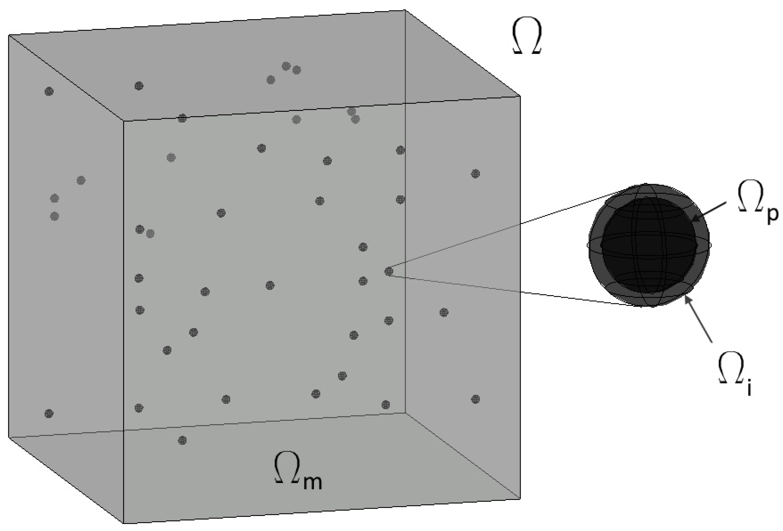
Figure 2.
Micro-structure composition of the composite under consideration.
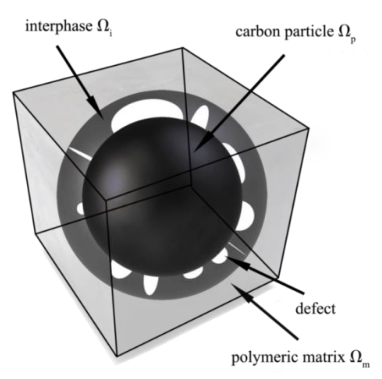
Figure 3.
Iso-parametric 20-noded 3D finite element: physical configuration—left graph, normalized local coordinate system—right graph.
Figure 3.
Iso-parametric 20-noded 3D finite element: physical configuration—left graph, normalized local coordinate system—right graph.

Figure 4.
Mesh of the RVE.

Figure 5.
Uniaxial stretch approximations for Laripur LPR 5020.
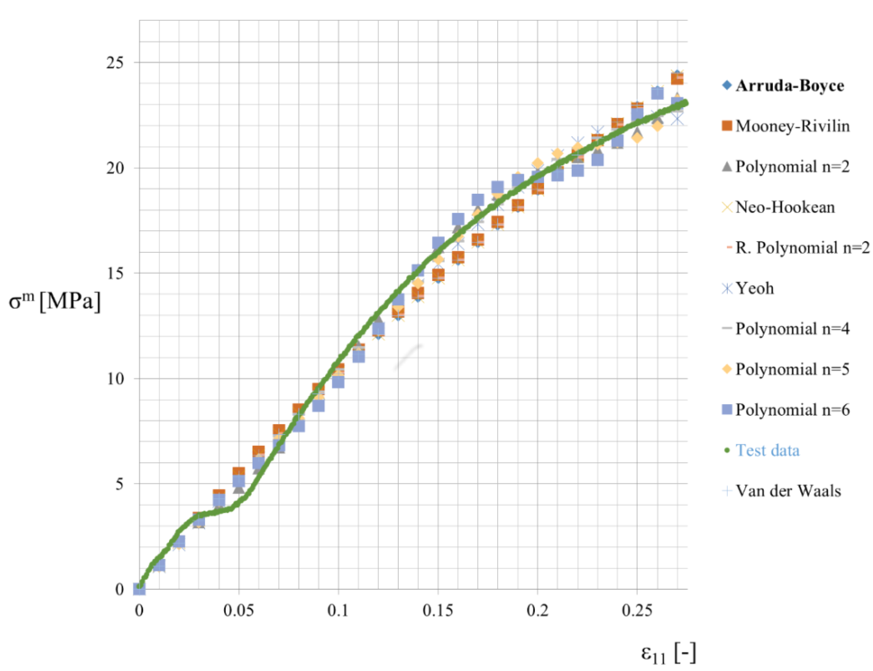
Figure 6.
Effective deformation energy of the composite.
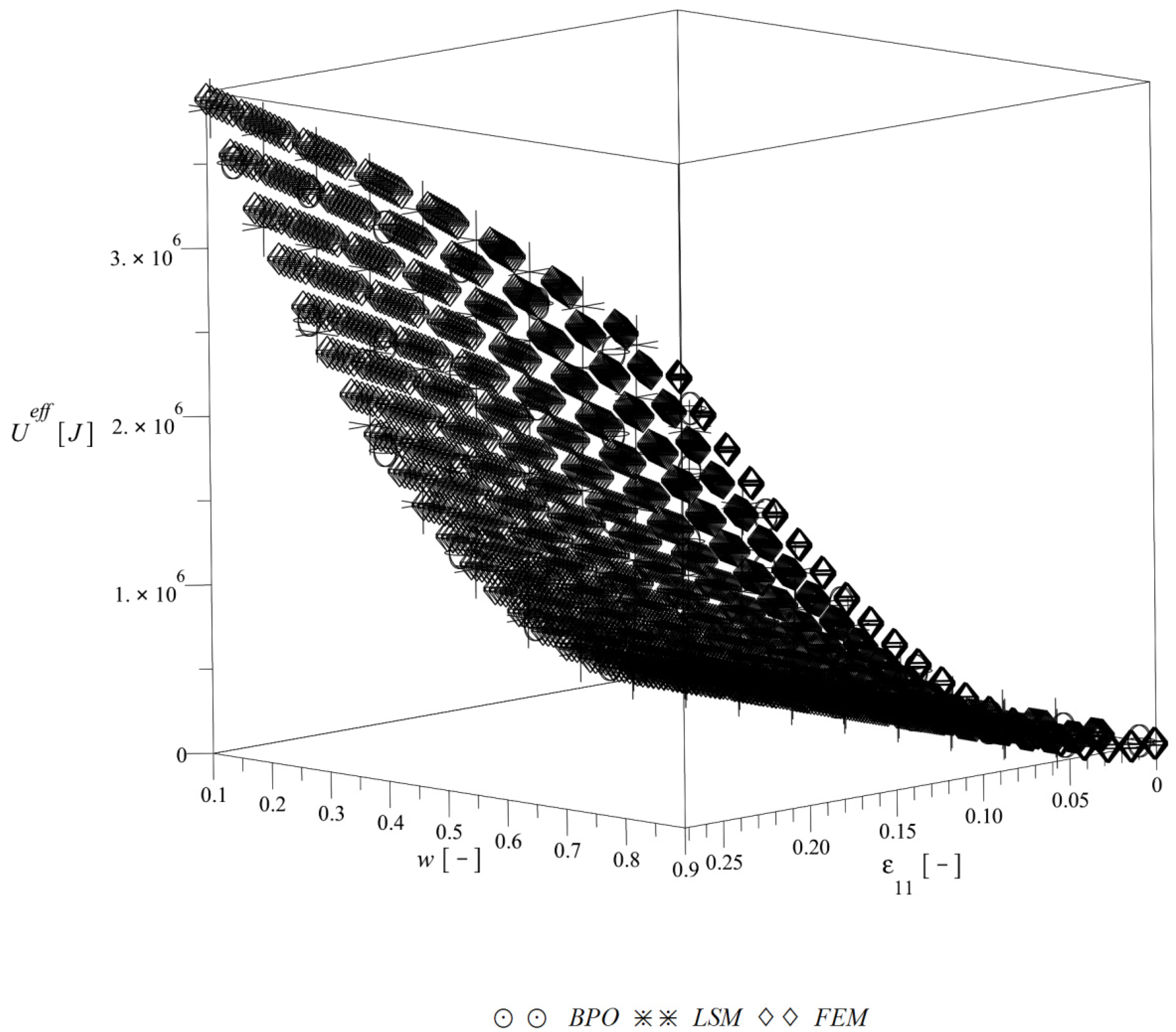
Figure 7.
Relative error of effective deformation energy approximations w.r.t. (a) the strain level and (b) the interface defects volume fraction .
Figure 7.
Relative error of effective deformation energy approximations w.r.t. (a) the strain level and (b) the interface defects volume fraction .

Figure 8.
Expected value of the effective deformation energy

Figure 9.
Coefficient of variation of the effective deformation energy .
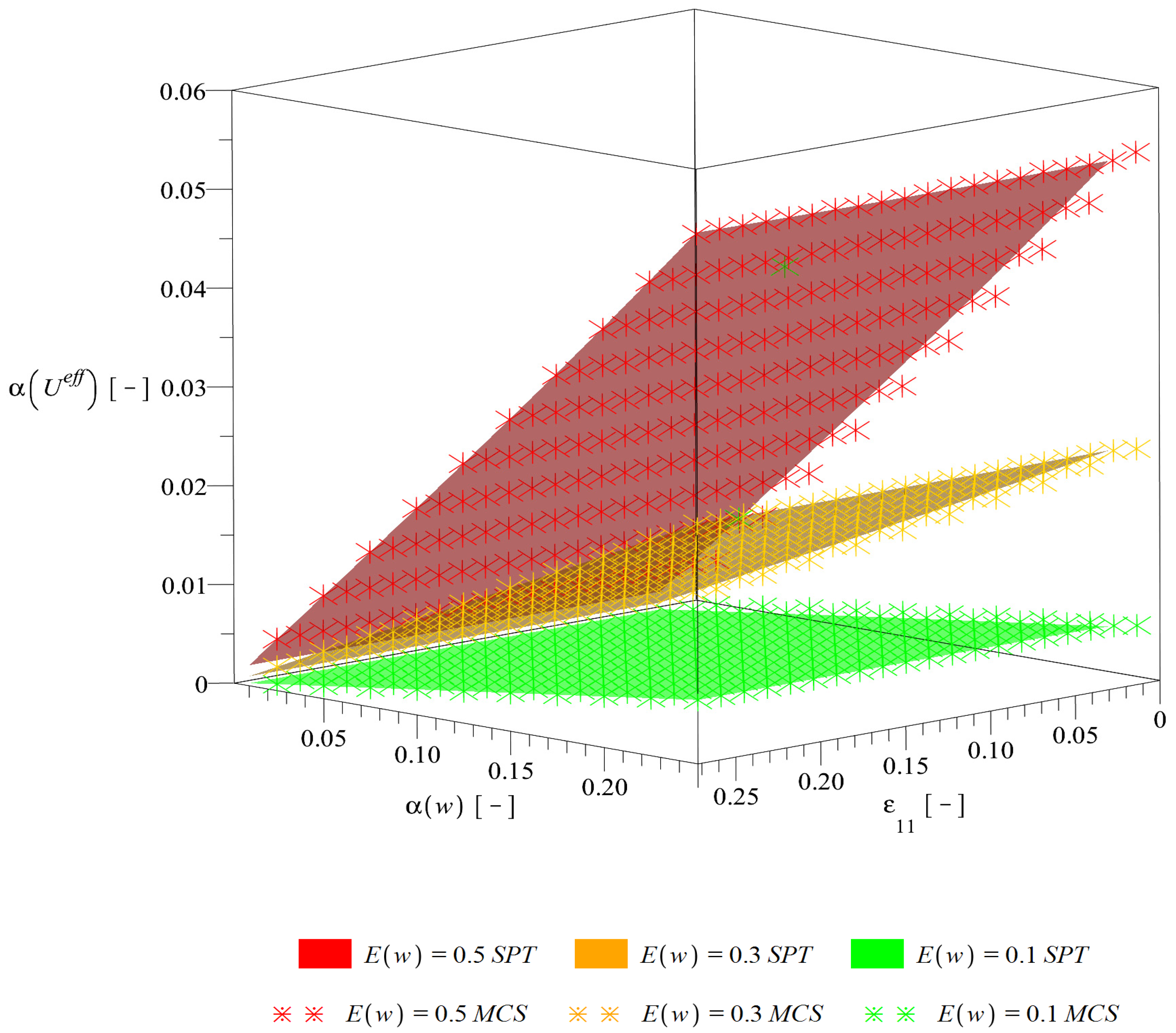
Figure 10.
Skewness of the effective deformation energy .

Figure 11.
Kurtosis of the effective deformation energy .

Table 1.
Elastic potentials for the selected hyper-elastic constitutive models.
| Constitutive Theory | Elastic Potential W |
|---|---|
| Neo–Hookean | , I1—the first invariant of the strain tensor, μ—shear modulus |
| Mooney–Rivlin | —empirical material constants, —the first and the second invariants of the left Cauchy-Green deformation tensor |
| Arruda–Boyce | |
| Yeoh | , —material constants |
| Van der Waals | , β—material parameter |
| Ogden | , , , —material constants, l1l2 are principal stretches |
© 2020 by the authors. Licensee MDPI, Basel, Switzerland. This article is an open access article distributed under the terms and conditions of the Creative Commons Attribution (CC BY) license (http://creativecommons.org/licenses/by/4.0/).
Share and Cite
MDPI and ACS Style
Sokołowski, D.; Kamiński, M.; Wirowski, A. Energy Fluctuations in the Homogenized Hyper-Elastic Particulate Composites with Stochastic Interface Defects. Energies 2020, 13, 2011. https://doi.org/10.3390/en13082011
AMA Style
Sokołowski D, Kamiński M, Wirowski A. Energy Fluctuations in the Homogenized Hyper-Elastic Particulate Composites with Stochastic Interface Defects. Energies. 2020; 13(8):2011. https://doi.org/10.3390/en13082011
Chicago/Turabian StyleSokołowski, Damian, Marcin Kamiński, and Artur Wirowski. 2020. "Energy Fluctuations in the Homogenized Hyper-Elastic Particulate Composites with Stochastic Interface Defects" Energies 13, no. 8: 2011. https://doi.org/10.3390/en13082011
Note that from the first issue of 2016, this journal uses article numbers instead of page numbers. See further details here.