Article

Bus Voltage Control of DC Distribution Network Based on Sliding Mode Active Disturbance Rejection Control Strategy

School of Electrical and Electronic Engineering, Tianjin University of Technology, Tianjin 300384, China
*
Author to whom correspondence should be addressed.
Energies 2020, 13(6), 1358; https://doi.org/10.3390/en13061358
Submission received: 10 January 2020 / Revised: 10 March 2020 / Accepted: 10 March 2020 / Published: 14 March 2020
(This article belongs to the Special Issue Advanced Control in Microgrid Systems)

Abstract

:
The DC distribution network has more advantages in power transmission, grid connection of distributed energy, and reliability of power supply when compared with AC distribution network, but there are still many problems in the development of DC distribution network. DC bus voltage control is one of the hot issues in the research of DC distribution network. To solve this problem, in this paper, a new type of sliding mode active disturbance rejection control (SMADRC) controller for AC/DC converters is designed and applied to the voltage outer loop. The linear extended state observer (LESO) can observe the state variables and the total disturbance of the system. The SMADRC is composed of a sliding mode controller, LESO, and disturbance compensator, which can compensate the total disturbance observed by LESO properly. Therefore, it improves the dynamic. At the same time, it can also reduce the system jitter that is caused by sliding mode controller. The state variables that are observed by the LESO are used in the design of sliding mode controller, which greatly simplifies the design of sliding mode controller. Finally, the simulation results of Matlab/Simulink show that the controller has good start-up performance and strong robustness.

Graphical Abstract

1. Introduction

In recent years, with the strong support of the government for distributed energy and the development of power electronics technology, increasing distributed energy sources (such as wind power generation, photovoltaic power generation and new energy vehicles) are connected to the power grid, as well as the popularization and promotion of many DC household electrical appliances and the wide application of industrial frequency conversion technology, which make the power supply and load composition of the distribution network change significantly [1,2,3]. The AC distribution network is facing many challenges, such as security, stability, and efficiency of power supply, because of the diversity and uncertainty of load and power supply. In response to this phenomenon, the concept of DC distribution network began to be put forward and gradually became a research hotspot.
Figure 1 shows the structure of DC distribution network. When compared with the AC distribution network, the DC distribution network has many advantages. On the one hand, the number and frequency of power electronic devices used in DC distribution network are less than that in AC distribution network. On the other hand, there is no eddy current loss in DC distribution network, which makes the DC distribution network have greater advantages in construction cost and transmission capacity. At the same time, the DC distribution network does not need to track reactive power and frequency, which will greatly improve the reliability and controllability of the system, and be more suitable for the access of distributed power [4].
Although DC distribution network has many advantages, it also faces many problems to be solved. Maintaining the voltage stability of DC bus is one of many problems. The load sudden change of DC distribution network and the three-phase voltage imbalance at the AC side will lead to the fluctuation of DC bus voltage. The bus voltage will exceed its normal working range if these disturbances are large enough, which will result in taking action of relay protection. If the situation is serious, it will lead to the system collapse, which will result in blackouts in large areas. Therefore, the study of DC distribution bus voltage stability has become a hot issue [5,6,7].
In view of this hot issue, many experts and scholars have conducted in-depth research. In reference [8,9,10], the AC-DC converter adopts the voltage and current double closed-loop control based on the traditional PI control strategy. Although the traditional PI controller has been widely used in industry, and achieved good control effect, it is difficult to achieve a good control effect in the face of DC distribution network. On the one hand, the control effect of PI controller largely depends on the precision of the mathematical model of the system, but, in the actual distribution network system, the AC-DC converter is strongly coupled and the load is time-varying, so it is difficult to establish the accurate mathematical model of the distribution network. Once the parameters of PI controller are set, they will not be changed. When the DC side load fluctuates in different degrees, it is difficult to ensure that the parameters of the PI controller are optimal. Therefore, the system under PI control has poor robustness. On the other hand, it is well known that the control principle of PI controller is to restrain the fluctuation of bus voltage through the deviation signal between the rated voltage and real-time bus voltage. In the actual DC distribution network, there are usually capacitor elements for suppressing the fluctuation of bus voltage. When the load power of DC side fluctuates, according to the principle of energy conservation (ignoring the power loss of power switch, that is, the energy input of AC side is equal to the energy absorbed by DC side), the power input of AC side should be immediately adjusted. However, the difference between the rated voltage and the real-time voltage of the bus is small, so that the voltage outer loop based on PI controller cannot make the appropriate response quickly, because the voltage at both ends of the capacitor cannot change suddenly, when the load power at the DC side changes suddenly. The current reference value of the current inner loop used to adjust the input power of the AC side is the output of the voltage outer loop. Therefore, the dynamic performance of the classical double closed-loop control strategy based on PI controller is poor, and the load disturbance will have a great impact on the system.
In reference [11,12], a fuzzy controller is designed to replace the PI controller of the voltage outer loop. The error e and the error change rate e ˙ of the voltage are taken as the input variables of the fuzzy controller, which are processed by fuzzy function and de fuzzy function to obtain the correction value. In reference [13,14], the error e and the error change rate e ˙ of the voltage are taken as the input variables of the fuzzy PI controller. The increment of the proportional gain Δ k p and the integral gain Δ k i are taken as the output variables of the fuzzy PI controller, which are used to modify the proportional gain k p and the integral gain k i of the PI controller, so as to improve the adaptability of the system. However, it still takes the deviation signal between the rated voltage and real-time bus voltage as its state variable. Therefore, it has not been able to overcome the response time delay that is caused by the voltage across the capacitor cannot be abruptly changed.
In response to the above-mentioned problem of the slow dynamic response of the voltage outer loop, a load current feedforward controller is added in reference [15,16,17] based on the voltage and current double closed loop. When the load changes suddenly, the load current feedforward control signal can quickly track the change of the load current and, together with the voltage outer loop control signal, can be used as the reference value of the current inner loop. The current of the AC-DC converter is quickly adjusted by the inner loop of the current loop, so that the input power can follow the change of the load power. This maintains the power balance between input and output and significantly improves the dynamic response speed of the system. However, this method needs to add additional current sensors, which increases the construction and maintenance costs of the system. When the DC bus is connected to multiple converter loads, multiple current transformers need to be installed, and the installation position of the current sensor becomes difficult. It is not conducive to the promotion of the DC distribution networks.
Sliding mode control is a kind of non-linear control. As it is not sensitive to system parameters and external disturbances, it has strong robust performance and a good control effect, especially for nonlinear time-varying nonlinear distribution networks. For this reason, many experts and scholars have made beneficial attempts on the application of sliding mode control in distribution networks. In reference [18], an integral term was added to the design of the sliding function in order to ensure that the system is located on or near the sliding surface in the initial state. This removes or reduces the time that is taken for the approach process, shortens the system startup time, and improves the rapidity of the system. Reference [19] introduced boundary layers on both sides of the sliding plane, which made the original discontinuous control variable continuous. This effectively reduces the chattering of the system and improves the control accuracy of the current, but it reduces the robustness of the system. Reference [20] used the second-order sliding mode control to suppress the fluctuation of bus voltage, and carried out experiments in actual physical systems. The results show that the second-order sliding mode control not only maintains the robustness of traditional sliding mode control, but also reduces the system jitter that is caused by the sliding mode control. Although the above sliding mode control reduces the chattering of the system and improves the starting characteristics of the system, they all take the deviation signal of voltage or current as the state variable of the sliding mode function. Therefore, it is difficult to overcome the time delay that is caused by the energy storage element. The dynamic performance of the system is hard to guarantee when the system is disturbed.
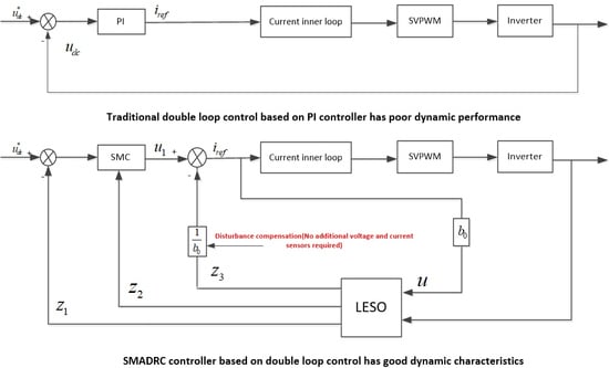
A sliding mode active rejection control controller is designed in this paper and applied to the voltage outer loop in view of the shortcomings of the above control strategies. The controller consists of a sliding mode controller, a linear expansion state observer, and a disturbance compensator. Its advantages lie in the following. Firstly, the sliding mode active disturbance rejection control (SMADRC) controller adds disturbance compensation when compared with the fuzzy controller and PI controller. When the load on the DC side of the distribution network abruptly changes, the disturbance compensator will respond quickly and be reflected in the reference current of the input current inner loop, together with the voltage outer loop control signal. Through the current inner loop, the incoming line current of the AC-DC converter is quickly adjusted, so that the input power can follow the change of the load power. Therefore, it avoids excessive charging and discharging of the capacitor, so that the bus voltage can be quickly stabilized, and the dynamic characteristics of the system are significantly improved. Secondly, when compared with adding load current feedforward controller based on double loop control, the controller that was designed in this paper does not need additional current sensor and control circuit. LESO can realize the observation and tracking of load current in the transient state, and the disturbance compensator, which reduces the difficulty of controller design and saves the cost of system construction and maintenance, properly compensates the observation value of LESO. Thirdly, when compared with the above-mentioned sliding mode control, the SMADRC controller that is designed in this paper still takes the voltage deviation signal as the state variable of the sliding mode function. The difference is that the LESO and disturbance compensator are added in this paper, which can not only reduce the chattering of the system and improve the control accuracy, but also improve the starting characteristics and anti-interference ability of the system. Finally, Matlab/Simulink simulation verify the authenticity and feasibility of the controller designed in this paper.

2. Mathematical Model of AC-DC Converter in DC Distribution Network

Figure 2 shows the circuit topology of the AC-DC converter. The following assumptions are be made in order to obtain a more concise mathematical expression of the AC-DC converter, combined with the actual power system:
(a)
The AC side power supply is an ideal three-phase power supply.
(b)
The AC side system is a symmetrical three-phase system.
(c)
The power switch is an ideal device, which has no transition process, no power loss, and no dead time effect.
In Figure 2, e a , e b , e c are equivalent AC power supply; i a , i b , i c are the AC side line current; R is the equivalent resistance of the filter; L is the equivalent inductance of the filter; C is the filter capacitance of DC side; U d c is the voltage at both ends of DC side capacitor; i d c is the current at both ends of DC side; i c is the current flowing through both ends of the capacitor; and, i L is the current flowing through both ends of the load. R L O A D is the equivalent load of DC distribution network.
S i = { 1 i   phase   upper   swith   is   on 0 i   phase   bottom   swith   is   on ,   i = a , b , c
Write the Kirchhoff voltage equation for nodes A, B and C in Figure 2, and Equation (2) can be obtained, as follows:
{ L d i a d t + R i a = e a ( U A N + U N O ) L d i b d t + R i b = e b ( U B N + U N O ) L d i c d t + R i c = e c ( U C N + U N O )
U N O is the voltage between node N and node O. Three-phase voltages ( U A N , U B N , U C N ) are related to the DC voltage ( U dc ) and three upper switching functions ( S a , S b , S c ), as shown in Equation (3):
{ U A N = S a U d c U B N = S b U d c U C N = S c U d c
Assume that the three-phase system on the AC side is balanced and there is no neutral line, the following Equation (4) can be obtained.
{ e a + e b + e c = 0 i a + i b + i c = 0 L d i a d t + L d i b d t + L d i c d t = 0 U A N + U B N + U C N = 0
According to Equations (2)–(4), voltage U N O can be expressed as in Equation (5).
U N O = U d c 3 i = a , b , c S i
Equation (6) can be obtained by writing Kirchhoff’s current equation for node M in Figure 2.
i d c C d U d c d t i L = 0
For the above system, there are always three power tubes that are on in normal operation, so there will be eight switching modes. The DC side current can be obtained, as shown in Equation (7):
i d c = i a S a S ¯ b S ¯ c + i b S ¯ a S b S ¯ c + i c S ¯ a S ¯ b S c + ( i a + i b ) S a S b S ¯ c + ( i a + i c ) S a S ¯ b S c + ( i b + i c ) S ¯ a S b S c + ( i a + i b + i c ) S a S b S c + 0 i a S a + i b S b + i c S c i L
Equation (8) can be obtained from Equations (6) and (7).
C d U d c d t = i a S a + i b S b + i c S c i L
To sum up, the mathematical model of DC distribution network can be expressed as Equation (9), as follows:
{ L d i a d t = e a R i a ( U d c S a U d c 3 i = a , b , c S i ) L d i b d t = e b R i b ( U d c S b U d c 3 i = a , b , c S i ) L d i c d t = e c R i c ( U d c S c U d c 3 i = a , b , c S i ) C d U d c d t = i a S a + i b S b + i c S c i L
The matrix form of Equation (9) can be obtained by Equations (10)–(14), as follows:
Z X ˙ = A ( t ) X + U
Z = [ L L L C ]
A ( t ) = [ R 0 0 U d c 3 i = a , b , c S i S a 0 R 0 U d c 3 i = a , b , c S i S b 0 0 R U d c 3 i = a , b , c S i S c S a S b S c 0 ]
X = [ i a i b i c U d c ] T
U = [ e a e b e c i L ] T

3. Classic Voltage and Current Double Closed Loop Control Based on PI Controller

The control strategy of the AC-DC converter is usually double closed-loop, namely current inner loop control and voltage outer loop control, which generally adopt the PI controller. When the system is in a stable state, the current inner loop control strategy can make the current phase consistent with the voltage phase, and realize the unit power rectification of the AC-DC converter. The output of the voltage outer loop is used as the given value of the current inner loop input. When the load power on the DC side changes, the current value of the current loop responds accordingly by continuously changing the given value. This realizes the tracking of the AC input power to the DC side load absorbed power.
According to Equation (9), the bus voltage of DC distribution network can be maintained as a constant value by adjusting the power switch of AC-DC converter and the AC side current. However, the control system design of AC-DC converter is difficult to achieve. On the one hand, the AC side current of AC-DC converter is always non-linear and time varying. On the other hand, the AC-DC converter itself is a multi-order nonlinear time-varying system. Therefore, it is necessary to transform the three-phase static coordinate system to the two-dimensional rotating coordinate system, whose rotating speed is the same as the fundamental frequency ω of the AC side power grid, in order to facilitate the design of the controller. Through coordinate transformation, the three-phase nonlinear time-varying alternating current in the static coordinate system can be transformed into the continuous current in the two-dimensional rotating coordinate system, which is more conducive to the design of the controller.
Three-phase static coordinate system is transformed into the coordinate of two-dimensional rotation (d–q) through the Park transformation matrix, as follows [21]:
T a b c / d q = 2 3 [ sin θ cos ( θ 120 ) cos ( θ + 120 ) sin θ sin ( θ 120 ) sin ( θ + 120 ) 0.5 0.5 0.5 ]
In matrix [ S d S q ] = T a b c / d q [ S a S b S c ] , θ is the angle between the a-axis in the three-phase phase stationary coordinate axis and the d-axis in the two-dimensional rotating coordinate axis.
Equation (16) is the mathematical model of AC side power supply in two-phase rotation coordinate (d–q), as follows:
[ e q e d e 0 ] = [ T a b c / d q ] [ e a e b e c ]
Matrix (17) is used to transform the (d–q) axis of two-phase rotation into the coordinate axis of two-phase static (α–β).
T d q / α β = [ cos θ sin θ sin θ cos θ ]
The mathematical model of t AC-DC converter circuit in two-dimensional rotation coordinates can be obtained by combining Equation (9) and Equation (16), as follows:
{ L d i d d t = e d R i d U d c S d + ω L i q L d i q d t = e q R i q U d c S q ω L i d C d U dc d t = 3 2 ( S d i d + S q i q ) i L
Assuming:
{ U d = S d U d c U q = S q U d c
The variables S d and S q are S a , S b , and S c in a two-dimensional rotating coordinate system.
The mathematical model of DC distribution bus voltage in two-dimensional rotating coordinate (d–q) can be obtained by substituting Equation (18) into Equation (19), as follows:
{ U d = e d R i d L d i d d t + w L i q U q = e q R i q L d i q d t w L i d
It can be seen from Equation (20) that there is coupling between voltage variable and current variable, which is not conducive to the design of the controller. Therefore, the feedforward decoupling control strategy is adopted to realize decoupling between voltage variable and current variable. When the PI controller is adopted in the current loop, the control law can be obtained in Equation (21), as follows:
{ U d = e d R i d + ω L i q k i p d ( i d * i d ) k i i d ( i d * i d ) d t U q = e q R i q ω L i d k i p q ( i q * i q ) k i i q ( i q * i q ) d t i d * = k u p ( U d c * U d c ) + k u i ( U d c * U d c ) d t
Variables ( e d , e q ) are the voltage of the phase voltage of the AC side power supply of the three-phase voltage type rectifier in the two-dimensional rotating coordinate axis; Variables ( U d , U q ) are the voltage of the AC side voltage of the three-phase voltage type rectifier in the two-dimensional rotating coordinate system; Variables ( i d , i q ) is the current of the AC side line current of the three-phase voltage type rectifier in the two-dimensional rotating coordinate system; Variables ( i d * , i q * ) are the current given in the two-dimensional rotating coordinate system value; k i p d and k i i d are d-axis proportional gain and integral gain in the current ring; k i p q and k i i q are the q-axis proportional gain and integral gain in current ring; U d c * is distribution network bus voltage rating; k u p and k u i are the proportional gain and integral gain in the voltage ring. When the three-phase grid is symmetrical, e d is a direct current with amplitude of E m and e q is equal to zero. When three-phase voltage and current are in phase, i d is a direct current with amplitude of I m and i q is equal to zero [22,23,24].
Figure 3 shows the control structure. The control system is composed of voltage outer loop, current inner loop, phase-locked loop, matrix conversion modules, and pulse signal generator. U d and U q are the output signal of PI controller, which are transformed into SVPWM recognizable signals after coordinate transformation. Subsequently, SVPWM sends control signals to the power switch tube, so as to realize the on or off of the power switch tube, which can realize the control of DC bus voltage.

Reason Analysis of Slow Dynamic Response of Classical Double Loop Control Based on PI Controller

When AC/DC bidirectional converter adopts double closed-loop control based on PI controller, its control block diagram can be obtained, as shown in Figure 4.
G v ( s ) is the closed-loop transfer function of the voltage loop; G i ( s ) is the open-loop transfer function of the current loop; U d c * ( s ) is the bus voltage of the branch frequency distribution network in the complex frequency domain; i L ( s ) is the load current of the DC distribution network in the complex frequency domain.
The relationship between U d c and i c in Figure 2 is Equation (22) (assume that the voltage across the capacitor at zero is zero).
U ( d c ) = 1 c 0 t i c d t
i c is the current flowing through both ends of the capacitor at time t .
According to Equation (22), the voltage change value Δ U ( d c ) from t 0 to t is Equation (23).
Δ U ( d c ) = 1 c t 0 t Δ i c d t
Equation (24) can be obtained by writing Kirchhoff’s current equation for node M, as in Figure 2.
i c = i d c i L
From Equation (24), when the load current ( i L ) changes, as long as i d c can track the change of i L well, it will not cause the change of i c . At the same time, it can be seen from Equation (23) that the fluctuation of the bus voltage is mainly caused by the change in current flowing across the capacitor.
Therefore, the fluctuation degree of the bus voltage mainly depends on whether i d c can track i L in time. It can be known that the value of i d c is mainly controlled by the current inner loop ( G i ( s ) ), and the current reference value ( i r e f ) of the current inner loop is the output value of the voltage outer loop G v ( s ) , according to Figure 4. As we all know, the traditional PI controller eliminates the fluctuation of the bus voltage based on the difference between the rated voltage and the real-time voltage of the bus. When the system is disturbed, the voltage difference will not change suddenly, because the voltage across the capacitor cannot be suddenly changed. Therefore, the PI controller based on error cannot respond quickly. This is the main reason why the dynamic response of the system is slow when PI controller is used in the voltage outer loop.

4. SMADRC Controller

Although the traditional PI controller has been widely used in industry and has good control effect, when the bi-directional AC-DC converter is started or the DC side load is suddenly changed, it is difficult for PI controller to ensure that the system has good dynamic quality according to the above.
A SMADRC controller is designed in this paper in view of the shortcomings of traditional PI controller. SMADRC controller consists of sliding mode controller, linear expansion state observer, and disturbance compensator. LESO is the heart of SMADRC controller. On the one hand, LESO can observe the state variables of the system. The observed state variables will be applied to the design of the sliding mode controller, which greatly simplifies the design of the sliding mode controller. On the other hand, LESO can also observe the total disturbance of the system. The observed total disturbance will be used in the design of the disturbance compensation link, which greatly improves the dynamic response of the system.

4.1. Introduction of Linear Extended State Observer

LESO is the core of linear active disturbance rejection control technology. LESO can estimate the state variables and the total disturbance of the system without giving an accurate mathematical model. For an n-order system with external interference, its expression is as follows:
y ( n ) = a n 1 y ( n 1 ) a n 2 y ( n 2 ) a 1 y ˙ a 0 y + ω + b u
In the above expression: y is the output of the system, u is the input of the system, ω is the unknown disturbance, the constants a 0 , a 1 , a n 1 are the structural parameters of the system, which might be unknown or partially known, and b is the controller gain. Let x 1 = y , x 2 = y ˙ x n = y ( n 1 ) , x n + 1 = f , f = a n 1 y ( n 1 ) a n 2 y ( n 2 ) a 1 y ˙ a 0 y + ω + ( b b 0 ) u . Suppose that f is differentiable. b 0 is the estimated value of b, b0b. The physical meaning of f is the total disturbance of the system, which consists of two parts: one is the uncertainty of the system itself and the other is the unknown disturbance of the outside the system. The disturbance f is extended to the (n + 1) state variable of the system. Subsequently, Equation (21) can be transformed into (n + 1) orders extended state space, which is described, as follows:
{ X ˙ = A X + B u + E f ˙ y = C X
In the above expression
X = [ x 1 x 2 x n x n + 1 ]
X ˙ = [ x ˙ 1 x ˙ 2 x ˙ n x ˙ n + 1 ]
A = [ 0 1 0 0 0 0 1 0 0 0 0 1 0 0 0 0 ] ( n + 1 ) × ( n + 1 ) B = [ 0 0 b 0 0 ] ( n + 1 ) × 1 E = [ 0 0 0 1 ] ( n + 1 ) × 1
C = [ 1 0 0 0 ] 1 × ( n + 1 )
The state variables of the above systems can be estimated by the following extended state observers:
{ Z ˙ = A X + B u + L ( y y ^ ) y ^ = C Z
The coefficient matrix A, B, C in Equation (31) is the same as that in Equation (26). Z is the state variable matrix of the extended state observer and Z ˙ is the derivative matrix of the state variable. L is the error feedback gain matrix of the observer to be designed. The expression of matrix L is as follows:
L = [ l 1 , l 2 l ( n + 1 ) ] T
The bandwidth ω 0 of the observer is introduced in reference in order to simplify the parameter design of matrix L [25]. Its expression is as follows:
s n + 1 + l 1 s n + + l n s + l n + 1 = ( s + ω 0 ) n + 1
The elements in matrix L can be determined, according to the property of identity, that is, the left and right sides of equal sign are equal.
{ l 1 = 3 ω 0 l 2 = 3 ω 0 2 l 3 = ω 0 3
When the system is asymptotically stable, the state variables of the system be traced by the state variables of the observer.
{ z 1 y z 2 y ˙ z n + 1 f
It can be seen from Equation (35) that, with the introduction of bandwidth, the original adjustment of parameters ( l 1 , l 2 l n ) of the LESO is changed to the adjustment of parameter ω 0 , which greatly simplifies the design of LESO. That is to say, the parameter ω 0 determines the whole performance of LESO. When the parameter ω 0 is larger, the bandwidth of LESO will be wider, which will lead to a higher tracking accuracy of LESO [26]. Therefore, the control effect of the controller will be better. However, there is usually noise in the actual system. The increase of ω 0 will improve the tracking accuracy of LESO, but it will also amplify the noise signal, which will affect the control quality of the controller.

4.1.1. The LESO Design of DC Distribution System

The expression of DC distribution bus voltage in two-dimensional rotating coordinate system is Equation (8). Equation (36) can be obtained by differential derivation of time on both sides of Equation (8).
d 2 U d c d t 2 = 3 2 L C k = d , q ( S k e k S k i k R ) 3 ω 2 C ( S q i d S d i q ) 3 2 L C k = d , q S k U k i ˙ L
Equation (37) can be obtained when the oriented voltage control [23] is adopted in the bus voltage control system of DC distribution network.
{ e q = 0 e d = E m i q = 0
E m is the effective value of the three-phase AC phase voltage.
Equation (38) can be obtained by bringing Equation (37) into Equation (36).
d 2 u d c d t 2 = 3 2 L C ( S d E M S d i d R ) 3 2 L C k = d , q S k U k 3 ω 2 C S q i d i ˙ L
Write Equation (38) in the form of state space, as shown in Equation (39):
{ [ x ˙ 1 x ˙ 2 x ˙ 3 ] = [ 0 1 0 0 0 1 0 0 0 ] [ x 1 x 2 x 3 ] + [ 0 0 b 0 0 0 1 ] [ u f ˙ ] y = x 1
In the above expression, b 0 = 3 ω / 2 C , the state variables ( x 1 , x 2 ) are the output voltage U d c and its differential U ˙ d c , x 3 = f is the total disturbance of the DC distribution network u = i d , f = 3 2 L C ( S d E M S d i d R ) 3 2 L C k = d , q S k U k i ˙ L + ( b b 0 ) u (Appendix A) According to the above description, the third-order LESO of the system can be obtained, as follows:
{ z ˙ 1 = z 2 3 ω 0 ( z 1 U d c ) z ˙ 2 = z 3 ω 0 2 ( z 1 U d c ) + b 0 u z ˙ 3 = ω 0 3 ( z 1 U d c )
According to the expression (40), if the parameter ω 0 is set, then the output variable ( z 1 , z 2 , z 3 ) of the third-order LESO can, respectively, track the bus voltage signal, differential signal of voltage, and the total disturbance of the system.

4.1.2. Convergence Proof of Third-Order LESO

Equation (41) is obtained by the Laplace transformation of Equation (40).
{ Z 1 ( s ) = ( 3 ω 0 s 2 + 3 ω 0 2 s + ω 0 3 ) ( s + ω 0 ) 3 U d c ( s ) + b 0 s ( s + ω 0 ) 3 i d ( s ) Z 2 ( s ) = ( 3 ω 0 2 s + ω 0 3 ) ( s + ω 0 ) 3 U d c ( s ) + b 0 ( s + 3 ω 0 ) ( s + ω 0 ) 3 i d ( s ) Z 3 ( s ) = ω 0 3 s 2 ( s + ω 0 ) 3 U d c ( s ) b 0 ω 0 3 ( s + ω 0 ) 3 i d ( s )
The tracking error of the third-order linear extended state observer is defined as in Equation (42).
{ e 1 = z 1 u d c e 2 = z 2 u ˙ d c e 3 = z 3 f
Equation (43) is obtained by the Laplace transformation of Equation (42)
{ E 1 ( s ) = b 0 s ( s + ω 0 ) 3 i d ( s ) s 3 ( s + ω 0 ) 3 U d c ( s ) E 2 ( s ) = b 0 s ( s + 3 ω 0 ) ( s + ω 0 ) 3 i d ( s ) + ( s + 3 ω 0 ) s 3 ( s + ω 0 ) 3 U d c ( s ) E 3 ( s ) = b 0 ( 1 ω 0 3 s 2 ( s + ω 0 ) 3 ) i d ( s ) ( 1 ω 0 3 ( s + ω 0 ) 3 ) s 2 U d c ( s )
In order to simplify the analysis, it can be assumed that i d and U d c are constant, then i d ( s ) and U d c ( s ) are equal to the following formula:
{ i d ( s ) = k 1 s U d c ( s ) = k 2 s
k 1 > 0 , k 2 > 0 . According to the classical control theory, Equation (45) shows the steady-state error expression of each state of the system.
{ e 1 s = lim s 0 s E 1 ( s ) = 0 e 2 s = lim s 0 s E 2 ( s ) = 0 e 2 s = lim s 0 s E 3 ( s ) = 0
It can be seen from Equations (42) and (45) that the third-order LESO can track the state variables and total disturbances of the DC distribution network well.

4.2. Design of Sliding Mode Controller

The rated voltage U d c r of the bus in the DC distribution network is a constant value, and U d c is the actual measured voltage of the DC bus. Subsequently, the tracking error is Equation (46).
e = U d c r U d c
Take differentiation on both sides of Equation (46) at the same time to get Equation (47).
e ˙ = U ˙ d c r U ˙ d c
Take differentiation on both sides of Equation (47) at the same time to get Equation (48).
e ¨ = U ¨ d c r U ¨ d c
Equation (49) can be obtained from Equation (40).
{ z 1 U d c z 2 U ˙ d c z 3 U ¨ d c b 0 u
In order to obtain good control effect, the differential signals of bus voltage error and voltage error in DC distribution network are selected as the state variables of the sliding mode function. Therefore, the sliding mode function is obtained as shown in Equation (50).
{ s = c e + e ˙ c > 0
Take differentiation on both sides of Equation (50) at the same time to get Equation (51).
s ˙ = c e ˙ + e ¨
The exponential reaching law is used to design the sliding mode controller in order to improve the control quality of the controller [27,28]. Take the sliding mode approach law as Equation (52) [29].
{ s ˙ = ε s i g n ( s ) k s ε > 0 k > 0
In the above equation, ε is the speed of the system state variable toward the sliding surface, if the value of ε is too small, then it will take a long time to converge from the initial state of the system to the sliding surface, but if the value of ε is too large, the state variable will produce obvious jitter on the sliding mode switching surface. K is the coefficient of exponential approach term. If the value of K is very large, the time from the initial position of the system state variable to the sliding surface will be shorter, but it will also reduce the area where the "sliding mode" exists. In general, in the process of parameter adjustment, if the ε is increased, then the k needs to be reduced in order to achieve good control effect [30,31].
The sliding mode control law can be obtained by simultaneous Equations (46)–(52).
u 1 = b 0 1 ( ε s i g n ( s ) + k s c z 2 z 3 )
The control rate u ( u = i r e f i r e f is the current inner loop reference value in Figure 2) of SMADRC controller is mainly composed of sliding mode control rate ( u 1 = b 0 1 ( ε s i g n ( s ) + k s c z 2 ) ) and disturbance compensator ( z 3 / b 0 ) by Equation (53). When the system is just started, the difference between the rated voltage of the bus and the real-time voltage of the bus is relatively large. At this time, the sliding mode controller in SMADRC controller plays the main role to ensure that the system has good startup characteristics. When the system is suddenly disturbed, the disturbance compensator will appropriately compensate according to the total disturbance that was observed by LESO. This will improve the dynamic quality of the system.
Figure 5 shows the SMADRC controller designed in this paper, which is composed of three order linear extended state observer, sliding mode controller, and disturbance compensator.
Figure 6 shows the application of SMADRC controller in the DC distribution network bus voltage control.

Proof of Reachability of Sliding Surface

Let Lyapunov function be Equation (54).
V = 0.5 s 2
According to Lyapunov’s second law [32], when the function value of the derivative function of V is less than or equal to zero, it meets the condition that the sliding mode can reach. Equation (55) shows the specific calculation formula.
d V d t = s d s d t = s ε s i g n ( s ) k s 2
Equation (56) can be got because of ε > 0 , k > 0 , s s i g n ( s ) 0 .
d V d t = s d s d t = s ε s i g n ( s ) k s 2 0
It can be seen from the above proof that the variable index approach rate meets the accessibility requirements. It can converge the initial point of the system to the sliding surface in a finite time in any state space.

5. Simulation Results and Analysis

The control variable analysis method is used, that is to say, only the voltage loop controller is different, the current loop controller uses PI controller, and whose parameters are the same, in order to evaluate the control effect of the SMADRC designed in this paper. The simulation experiment is completed with Matlab/Simulink. Table 1 gives the system parameters and Table 2 provides the controller parameters. Figure 7 shows the system structure used in the simulation experiment.
Figure 8 shows the overall control effect diagram of the two controllers during the simulation period. It can be seen from the effect diagram that, when compared with the traditional PI controller, the SMADRC controller designed in this paper has greater advantages in the starting, PV grid-connected, load mutation, and steady state characteristics. Next, this paper will compare the two kinds of controllers from the following five situations: starting characteristics, load mutation, PV grid-connected, three-phase voltage imbalance, and transient three-phase current.
Figure 9 shows the waveform change of the bus voltage in the DC distribution network during the start-up of the AC-DC converter. On the one hand, as we all know, the value of the proportional gain affects the speediness and overshoot of the PI controller. The larger the proportional gain is, the better the speediness and overshoot of the system will be. It can be seen from Figure 9 that the rise time of the system under the control of the two controllers is the same, but the overshoot of the system under the control of PI controller is larger than that under the control of SMADRC. If we want to continue to improve the rise time of the system under the control of PI controller, we need to increase the proportional gain, but this will cause the overshoot of the system to become larger. On the other hand, it can be seen from Figure 9 that, when the bus voltage of DC distribution network under SMADRC control reaches the rise time, it will quickly stabilize near the rated voltage, but the system under PI controller control will need a long transition process to stabilize near the rated voltage. In conclusion, the AC-DC converter that is controlled by SMADRC has better starting performance and transient performance.
At 0.3 s, the resistive load of the DC distribution network was suddenly reduced to half of the original and, at 0.9 s, the constant power load of the DC distribution network was suddenly reduced to half of the original, which will lead to a transition process of the system. It can be seen from Figure 10 that, on the one hand, the maximum amplitude variation of bus voltage in DC distribution network controlled by SMADRC controller is about half of that under PI controller. On the other hand, the system transition time under SMADRC controller is much shorter than that under the PI controller. Therefore, SMADRC controller has stronger robust performance than PI controller.
At 0.5 s, the photovoltaic is connected to the power grid and, at 0.7 s, the light intensity changes from the original 1000 W/m2 to 100 W/m2. The corresponding bus voltage diagrams are Figure 11a,b, as in Figure 10. It can be seen from Figure 11a that, when the PV is connected to the grid, the SMADRC controller has slightly better control performance than the PI controller. However, when the light intensity suddenly decreases, the SMADRC controller’s control effect is much better than the PI controller. The maximum bus voltage fluctuation under SMADRC controller is approximately half of the PI controller. Accordingly, when compared to PI controllers, the SMADRC controllers are more suitable for distribution networks with distributed power.
At 1.1 s, the three-phase voltage is not symmetrical and, at 1.2 s, the three-phase voltage becomes symmetrical three-phase voltage again. Figure 12 shows the waveform diagram. Figure 13 shows the corresponding bus voltage. It can be seen from Figure 13 that the SMADRC controller has better robustness than the PI controller when the three-phase imbalance occurs in the AC power supply. When the three-phase imbalance disappears, the SMADRC controller can return to the equilibrium point faster.
It can be seen from Figure 14 that the SMADRC controller has no effect on the current inner loop controller. The PI controller of current inner loop can make the current phase of AC side track the voltage phase and realize unit power rectification. The control effect of the two controllers is almost the same from this point of view.
Figure 15 illustrates the current waveform change diagram of the AC side of the DC distribution network with different controllers. When the system is in steady state, its waveforms are sine wave. When the time is 0.3 s, the load side of the DC distribution network suddenly changes to the original half. The system will have a transient process because of the existence of inductance and capacitance. However, the transient time of the system with SMADRC controller is less than that of the system with PI controller.

6. Conclusions

The SMADRC controller that is designed in this paper consists of sliding mode controller, LESO, and disturbance compensator. The LESO can track the total disturbance of the system without adding additional current transformers. Subsequently, the disturbance compensator appropriately compensates the total disturbance observed by the observer, which improves the dynamic performance of the system. At the same time, the LESO can also observe the state variables of the system. The observed values are applied to the design of the sliding mode controller, which simplifies the design of the sliding mode controller. The sliding mode controller guarantees a good starting performance of the system. Finally, numerical simulation verifies its performance. The simulation results show that the SMADRC controller that is designed in this paper can effectively suppress the bus voltage fluctuation, significantly shorten the bus voltage fluctuation time, and is more conducive to distributed power supply. At the same time, because it does not require information transmission between devices to suppress bus voltage fluctuations, it is more conducive to plug and play of the load. Finally, the SMADRC that is designed in this paper can control the system without knowing the specific mathematical model of the system, so it has strong portability. It provides a new design idea for other systems that are difficult to build accurate mathematical models.

Author Contributions

X.Z. conceived the main idea for the proposed LADRC and performed overall analysis; B.W. wrote this paper; Y.M. contributed to analyzing the experimental results. All authors have read and agreed to the published version of the manuscript.

Funding

This work was funded by National Natural Science foundation of China (NO. 51877152) and Natural Science Foundation of Tianjin of China (NO. 18JCZDJC97300).

Acknowledgments

The authors are grateful to the support by the National Natural Science foundation of China (NO. 51877152), Natural Science Foundation of Tianjin of China (NO. 18JCZDJC97300) and Tianjin University of Technology for their support.

Conflicts of Interest

The authors declare no conflict of interest.

Abbreviations

LESOLinear Extended State Observer
SMADRCSliding Mode Active Disturbance Rejection Control
SVPWMSpace Vector Pulse Width Modulation
MPPTMaximum Power Point Tracking
SMCSliding Mode Control

Appendix A

Differentiable description of f in line 356.
f contains a switching function, so it also gives the illusion that f cannot be differentiable, but the switching function is differentiable. Its differentiation is an impact function, and the differential of an impulse function is an impact even function. On the other hand, in the actual power system, there are inductance devices in the AC measurement, so there is no disconnection phenomenon. That is to say, if a more accurate mathematical model is established in the actual system, the differentiation of f will be easier to know. The design of LESO does not need to know the specific expression of f , but only needs to know that f can be differentiated.

References

  1. Yoldas, Y.; Onen, A. Enhancing smart grid with microgrids: Challenges and opportunities of the article. Abbreviated Renew. Sustain. Energy Rev. 2017, 72, 205–214. [Google Scholar] [CrossRef]
  2. Prabhala, V.A.; Baddipadiga, B.P. An Overview of Direct Current Distribution System Architectures & Benefits of the article. Abbreviated Energy 2018, 11, 2463. [Google Scholar]
  3. Arunkumari, T.; Indragandhi, V. An overview of high voltage conversion ratio DC-DC converter configurations used in DC micro-grid architectures of the article. Abbreviated Renew. Sustain. Energy Rev. 2017, 77, 670–687. [Google Scholar] [CrossRef]
  4. Wang, C.; Li, W.; Wang, C.; Meng, Z.; Yang, L. Summary of classification and suppression methods of bus voltage fluctuation in DC microgrid. Chin. J. Electr. Eng. 2017, 37, 84–98. [Google Scholar]
  5. Wu, B.; Xie, W.; Ye, H. DC bus voltage stability control technology of AC/DC hybrid microgrid. China Power 2017, 50, 62–66. [Google Scholar]
  6. Li, X.; Wang, C.; Guo, L.; Zhou, L.; Feng, Y. Summary of research on Key Technologies of DC micro grid stability control. Power Supply 2015, 32, 1–14. [Google Scholar]
  7. Kang, Z.; Chen, X.; Cui, C.; Yu, H. Bus voltage control of DC distribution network based on ESO and terminal sliding mode control. Chin. J. Electr. Eng. 2018, 38, 3235–3243. [Google Scholar]
  8. Shimizu, T.; Jin, Y.; Kimura, G. DC ripple current reduction on a single-phase PWM voltage-source rectifier. IEEE Trans. Ind. Appl. 2000, 36, 1419–1429. [Google Scholar] [CrossRef]
  9. Li, P.; Dong, Y.; Duan, K.; Wu, W. Simulation Research on control strategy of bi-directional AC/DC converter parallel system in DC microgrid. Power Syst. Prot. Control 2017, 45, 43–50. [Google Scholar]
  10. Ma, H.; Xu, D. Passive filtering technology to eliminate the influence of long cable of PWM inverter driven AC motor. J. Electr. Technol. 2001, 6, 1–3. [Google Scholar]
  11. Guo, Q.; Yuan, S.; Zhou, C.; Wang, H.; Wang, X. Research on Microgrid Smooth Switching Control Strategy Based on Fuzzy Control. High Volt. Eng. 2015, 41, 3281–3287. [Google Scholar]
  12. Wang, S.; Chen, S.; Zhao, W. A fuzzy control method for three-phase voltage regulator of intelligent distribution network. Autom. Electr. Power Syst. 2016, 40, 72–80. [Google Scholar]
  13. Zheng, Z.; Wang, N.; Sun, Z. Fuzzy PI Compound Control of PWM Rectifiers with Applications to Marine Vehicle Electric Propulsion System. Int. J. Fuzzy Syst. 2018, 20, 587–596. [Google Scholar] [CrossRef]
  14. Yang, X.; Fang, J.; Liu, C. Research on three-phase PWM rectifier based on fuzzy adaptive control. Comput. Technol. Autom. 2017, 36, 29–32 + 45. [Google Scholar]
  15. Jiang, S.G.; Wang, W.; Wang, P.B.; Liu, G.H. Power-feedforward-based control strategy of grid-connected single-phase PV system. Electr. Power Autom. Equip. 2010, 30, 16–19. (In Chinese) [Google Scholar]
  16. Li, X.; Guo, L.; Feng, Y. A nonlinear disturbance observer based DC bus voltage control for a dc microgrid. Proc. CSEE 2016, 36, 350–359. (In Chinese) [Google Scholar]
  17. Li, S.; Li, Y.; Chen, R. Study of the optimum feed-forward control strategy in back-to-back converter system. Proc. CSEE 2006, 26, 74–79. (In Chinese) [Google Scholar]
  18. Baghaee, H.R.; Mirsalim, M.; Gharehpetian, G.B.; Talebi, H.A. A decentralized power management and sliding mode control strategy for hybrid AC/DC microgrids including renewable energy resources. IEEE Trans. Ind. Inform. 2017, 1–12. [Google Scholar] [CrossRef]
  19. Morstyn, T.; Savkin, A.V.; Hredzak, B.; Agelidis, V.G. Multi-agent sliding mode control for state of charge balancing between battery energy storage systems distributed in a DC microgrid. IEEE Trans. Smart Grid 2017, 9, 4735–4743. [Google Scholar] [CrossRef]
  20. Cucuzzella, M.; Lazzari, R.; Trip, S.; Rosti, S.; Sandroni, C.; Ferrara, A. Sliding mode voltage control of boost converters in DC microgrids. Control Eng. Pract. 2018, 73, 161–170. [Google Scholar] [CrossRef]
  21. Li, S.; Li, Y.; Sun, J.; Jin, Q.; Li, X. Power quality control method of micro grid based on control strategy of inverter distributed power supply. Grid Technol. 2010, 34, 6–11. [Google Scholar]
  22. Zhu, X. Research on Grid Voltage Oriented Three-Phase Grid Connected Inverter; Nanjing University of Aeronautics and Astronautics: Nanjing, China, 2010. [Google Scholar]
  23. Fan, Z. Research on Low Voltage Ride through Control Strategy of Photovoltaic Grid Connected Power Generation System; Tianjin University of Technology: Tianjin, China, 2019. [Google Scholar]
  24. Gao, Z. Scaling and bandwidth-parameterization based control tuning. In Proceedings of the American Control Conference, Denver, CO, USA, 4–6 June 2003; pp. 4989–4996. [Google Scholar] [CrossRef]
  25. Yuan, D.; Ma, X.; Zeng, Q.; Qiu, X. Frequency band characteristics and parameter configuration of linear ADRC for second-order systems. Control Theory Appl. 2013, 30, 1630–1640. [Google Scholar]
  26. Chen, K.; Cao, Y.; Jiang, Y. Fuzzy PI control strategy of three-phase grid connected inverter based on grid voltage vector directional control. J. Shanghai Electr. Power Univ. 2017, 33, 55–59. [Google Scholar]
  27. Zhang, L.; Su, Y.; Wang, H. A nonsingular fast terminal sliding mode control with an exponential reaching law for robot manipulators. Proc. Inst. Mech. Eng. 2019, 233, 1575–1587. [Google Scholar] [CrossRef]
  28. Devika, K.B.; Thomas, S. Power rate exponential reaching law for enhanced performance of sliding mode control. Int. J. Control Autom. Syst. 2017, 15, 2636–2645. [Google Scholar]
  29. Rahman, M.H.; Saad, M.; Kenné, J.P.; Archambault, P.S. Control of an exoskeleton robot arm with sliding mode exponential reaching law. Int. J. Control Autom. Syst. 2013, 11, 92–104. [Google Scholar] [CrossRef]
  30. Liu, J.; Sun, F. Research and development of sliding mode variable structure control theory and algorithm. Control Theory Appl. 2007, 24, 407–418. [Google Scholar]
  31. Luo, X.; Zhu, Z.; Guan, X. Chattering weakening adaptive sliding mode control for nonlinear time-delay systems. Control Decis. 2009, 24, 1429–1431 + 1435. [Google Scholar]
  32. Chekroun, A.; Frioui, M.N.; Kuniya, T.; Touaoula, T.M. Global stability of an age-structured epidemic model with general Lyapunov functional. Math. Biosci. Eng. 2019, 16, 1525–1553. [Google Scholar] [CrossRef]
Figure 1. System structure of DC distribution network.
Energies 13 01358 g001
Figure 2. AC-DC converter circuit topology.
Energies 13 01358 g002
Figure 3. Control structure of the system using PI controller.
Energies 13 01358 g003
Figure 4. Double closed loop control block diagram based on PI controller.
Energies 13 01358 g004
Figure 5. Sliding mode active disturbance rejection control (SMADRC) controller.
Energies 13 01358 g005
Figure 6. Application of SMADRC controller in DC distribution network bus voltage control.
Energies 13 01358 g006
Figure 7. System structure.
Energies 13 01358 g007
Figure 8. The overall control effect of the two controllers during the simulation period.
Energies 13 01358 g008
Figure 9. DC voltage during the start-up.
Energies 13 01358 g009
Figure 10. DC voltage during the load transients: (a) Resistance type load and (b) Constant power load.
Energies 13 01358 g010
Figure 11. Impact of photovoltaic on bus voltage: (a) Photovoltaic connection to the grid and (b) Sudden decrease in light intensity.
Energies 13 01358 g011
Figure 12. Three-phase voltage.
Energies 13 01358 g012
Figure 13. Bus voltage.
Energies 13 01358 g013
Figure 14. Grid voltage and current of phase A: (a) PI controller and (b) SMADRC controller.
Energies 13 01358 g014
Figure 15. Three-phase grid currents during the load transients. (a) PI controller (b) SMADRC controller.
Energies 13 01358 g015
Table 1. System parameters.
SubsystemParameterValue
AC system parametersPhase voltage380 V
Source voltage frequency50 Hz
AC-DC converterFilter inductance at AC side0.003 H
Filter resistance at AC side0.1 Ω
Sample time5 × 10−6 s
DC bus capacitor0.008 F
Bus capacitor initial voltage500 V
Photovoltaic DC-DC converter parametersSample time5 × 10−6 s
Energy storage inductor0.005 H
Energy storage capacitor0.000162 F
DC-AC converterSample time5 × 10−6 s
Filter inductor0.0001 H
Filter capacitor0.0023 F
DC side loadRated DC constant power load3000 W
Rated DC resistance load40 Ω
Rated AC resistive load80 Ω
Bus rated voltage700 V
Table 2. Controller parameters.
ParameterValue
Sliding Mode Controller Parameters/ c 100
Sliding Mode Controller Parameters/ k 180
Sliding Mode Controller Parameters/ ε 110
Observer Bandwidth/ ω 0 460
Observer Bandwidth/ b 0 19,625
Outer Loop PI Controller Parameters/ k u p 1.1
Outer Loop PI Controller Parameters/ k u i 45
Inner Loop PI Controller Parameters/ k i p d 20
Inner Loop PI Controller Parameters/ k i i d 120
Inner Loop PI Controller Parameters/ k i p q 20
Inner Loop PI Controller Parameters/ k i i q 100

