T2FL: An Efficient Model for Wind Turbine Fatigue Damage Prediction for the Two-Turbine Case


Technical University of Denmark, Department of Wind Energy, Frederiksborgvej 399, 4000 Roskilde, Denmark
*
Author to whom correspondence should be addressed.
Energies 2020, 13(6), 1306; https://doi.org/10.3390/en13061306
Submission received: 20 December 2019
/
Revised: 3 March 2020
/
Accepted: 5 March 2020
/
Published: 11 March 2020
(This article belongs to the Special Issue Lifetime Extension of Wind Turbines and Wind Farms)
Abstract
:Wind farm load assessment is typically conducted using Computational Fluid Dynamics (CFD) or aeroelastic simulations, which need a lot of computer power. A number of applications, for example wind farm layout optimisation, turbine lifetime estimation and wind farm control, requires a simplified but sufficiently detailed model for computing the turbine fatigue load. In addition, the effect of turbine curtailment is particularly important in the calculation of the turbine loads. Therefore, this paper develops a fast and computationally efficient method for wind turbine load assessment in a wind farm, including the wake effects. In particular, the turbine fatigue loads are computed using a surrogate model that is based on the turbine operating condition, for example, power set-point and turbine location, and the ambient wind inflow information. The Turbine to Farm Loads (T2FL) surrogate model is constructed based on a set of high fidelity aeroelastic simulations, including the Dynamic Wake Meandering model and an artificial neural network that uses the Bayesian Regularisation (BR) and Levenberg–Marquardt (LM) algorithms. An ensemble model is used that outperforms model predictions of the BR and LM algorithms independently. Furthermore, a case study of a two turbine wind farm is demonstrated, where the turbine power set-point and fatigue loads can be optimised based on the proposed surrogate model. The results show that the downstream turbine producing more power than the upstream turbine is favourable for minimising the load. In addition, simulation results further demonstrate that the accumulated fatigue damage of turbines can be effectively distributed amongst the turbines in a wind farm using the power curtailment and the proposed surrogate model.
1. Introduction
Wind turbines are typically designed for specific wind conditions that satisfy the requirements defined by the IEC standards [1]. In a wind farm, wind turbines are usually grouped together, and the performance of the turbines in power and loads are affected significantly by the turbine aerodynamic wake interactions. For example, downstream wind turbines are typically subjected to the wake generated by upstream turbines, and this wake effect causes power loss and additional fatigue to the downstream turbines. Thus, site-specific assessments, including simulations over many design load cases, need to be conducted. Such turbine load calculations, which take into account the inflow wind condition and wind direction in a wind farm, typically require Computational Fluid Dynamics (CFD), which are computationally expensive. This motivates the development of methods and procedures for simplifying load assessments.
A variety of engineering models has been developed to facilitate the simplification of the wind farm load assessment. One of the early models was developed by Sten Frandsen [2]. It maps the wake effects to an equivalent ambient turbulence level. This fictitious turbulence causes the same level of fatigue load accumulation as the actual wind-induced turbulence for the downstream turbines. The Sten Frandsen approach is widely used due to its simplicity; however, some studies suggested that the load assessment by the method is often conservative [3]. A later developed more advanced engineering approach, the Dynamic Wake Meandering (DWM) model [4], includes the wake velocity deficit, meandering dynamics and added wake turbulence in a wind field for aeroelastic load simulations. This engineering model can predict the wake-induced load effects very well and has been validated in numerous studies [5,6]. To further simplify the wind farm load assessment, a surrogate-model-based approach became popular, for example [7,8,9], where the model contains the fatigue loads and statistics from a large number of aeroelastic simulations, including various wind speeds, turbulence intensities and wake profiles. For example, [8] developed a model that maps the wake properties into wind turbine loads, whilst a study by [9] proposed the development of a surrogate model that captures the turbine fatigue in considerations of numerous yaw and inflow conditions.
The majority of surrogate model studies focus on relating the wind inflow and wake information to the turbine fatigue loads. However, the turbine operating condition, such as down-regulation, would also impact upon the fatigue of the downstream turbines. Therefore, the aim of this work is to define and demonstrate a procedure that constructs a simplified and efficient surrogate model to map the turbine operating condition together with the wind inflow information to the fatigue loads of a wind farm. The proposed Turbine to Farm Loads (T2FL) surrogate model produces a quick load assessment for a wind farm, allowing a number of applications, such as wind farm layout optimisation, turbine lifetime estimation and wind farm control.
The remainder of this paper is organised as follows. In Section 2, the model development is presented together with the input variables and its limits. In addition, the framework used for the simulations is discussed together with the data set used to train the surrogate models. The verification of the surrogate model is demonstrated in Section 3. In Section 4, applications of the proposed surrogate model on wind farm fatigue studies and wind farm control are discussed. Finally, it is followed by conclusions in Section 5.
2. Methodology: Surrogate Model Development
2.1. Selection of Input Variables And Limits
2.1.1. Input Parameters
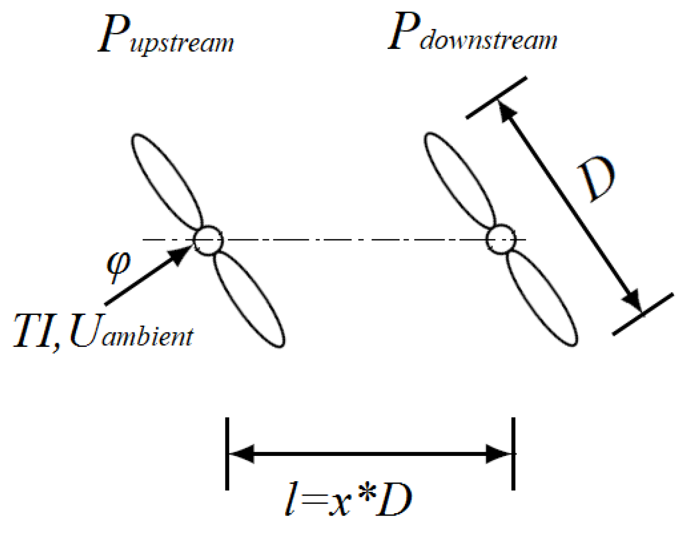
First, the factors that influence the turbine loads in a wind farm need to be identified. In order to identify the important factors, without loss of generality, a farm with two wind turbines (WTs) is considered (Figure 1). The turbine diameter is D, and its interspace l is given as a function of the diameter. The most important external factors with direct impact on the WT loading are the inflow wind characteristics:
- Ambient wind speed (),
- Ambient wind direction (),
- Ambient wind turbulence intensity ().
The wind direction in combination with the upstream WT wake alters the operation of the downstream one. The latter can operate under a full-to-no wake situation. Other wind characteristics, such as the wind shear and stability of the atmosphere, are not considered as variables in this study.
The two wind turbine array can be parameterised by the distance l between the turbines (WT interspace) as a function of rotor diameter. Furthermore, the power output level on each WT, in other words, the power down-regulation, is also considered as a parameter. Down-regulation becomes important in wind farms nowadays with high wind penetration in the electric grid mixture. The operators are asked to produce a certain amount of power to keep the grid stable or provide ancillary services, such as frequency control and reserve power [10]. The authors have performed a study on the impact on wind turbine loads from different down-regulation control strategies [11] on a downstream WT within a wind farm. It was based on aeroelastic simulations and has shown how the fatigue loads change as a function of down-regulation percentage as well as the changes between different control strategies. Here, the most commonly used strategy from the turbine manufacturers is considered. It is called induction control and the WT constrains its power output by pitching the blades to feather after the rated rotor speed has been reached. The WT power output control set point leads to these parameters:
- Derating percentage of Upstream WT (),
- Derating percentage of Downstream WT ().
where the power output for each WT (, ) is constrained to the desired level as a function of nominal WT power (Equation (1)):
2.1.2. Input Space
Next, the boundaries of the parameter space need to be defined. For the ambient wind speed, the range from WT cut-in to cut-out operation is considered, typically 3 to 25 m/s. The ambient turbulence intensity (TI) varies between offshore and onshore wind farms; thus, a wide range is included. The , which is observed at offshore farms, is selected as the lowest value. The selection is based on published measurements on real wind farms. The authors of [12] have reported minimum ambient TI measurements on the Greater Gabbard offshore wind farm of around . Similar met-mast measurements have been reported for the Horns Rev 1 and Lillgrund offshore wind farms in the study of [13]. In this study, the highest value is set to , which can be found in complex onshore terrain [14]. The turbulence is stochastic in nature; therefore, more than one realisation per case should be simulated for robust statistics and consistent load prediction. The IEC standard proposes to run six realisations per case; however, in this study, four are used as a compromise between accuracy and efficiency.
The wind turbine interspace is dependent solely on the farm layout. In this analysis, the minimum turbine distance of is considered, which covers even tight wind farm layouts, for example, the Lillgrund wind farm with a minimum wind turbine inter-spacing of [13]. The maximum value is taken as in order to be conservative since the authors do not have a specific reference of the maximum distance that the wake will affect the downstream WT depending on the wind conditions. The interspacing is considered at diameters of 3, 5, 7, 9 and 20.
The incoming wind direction together with the WT interspace determines if the downstream turbine is under full, partial or no wake situation. The authors of [7] have observed that for an incoming wind direction of 18 degrees or higher with WT inter-spacing, the wake effect on the downstream WT fatigue damage is negligible. In order to be conservative, the upper value is set as 22 degrees. It was also shown that the load level at full wake (0 degrees) and small angle steps around 0 degrees, such as from 0 to 2 degrees case, alters the load levels significantly, thus, a fine discretisation angle of 2 degrees should be used around that range. Thus, from zero to ten degrees, a step of two is considered, and afterwards, the step is set to four degrees.
Finally, for the WT power output constraints, the boundaries are set to no down-regulation () and up to curtailed. For example, WT down-regulation indicates the shut down of a WT, which can also be analysed using the proposed method. In this case, the non-operating WT is neglected and the inter-spacing between the ‘new’ pair of operating WTs is considered. The wind speed and the de-rating variables are uniformly distributed in the input space.
Table 1 summarises the input variables and spaces. After identifying the relevant parameter space, which in this case there are six parameters, the aeroelastic simulations can be defined. A WT model needs to be selected, and typical ten minute aeroelastic simulations are performed using aeroelastic code HAWC2 (Horizontal Axis Wind turbine simulation Code 2nd generation) [15]. The short term (1 Hz) fatigue loads are computed based on the rain-flow counting algorithm [16]. Depending on the material, a Wöhler exponent is selected. Typical values are 4, for construction steel, which is used in most of the turbine towers, and 12 for composite materials, such as the blade.
The outcome of the aeroelastic simulations is then organised in a database, and a surrogate model is generated for every output of interest. The T2FL surrogate model is quite general thus powerful and can be used for both optimisations of wind farm layouts or real-time wind farm control based on WT fatigue loads. For instance, fatigue load alleviation or redistribution on a WT level or global load minimisation in a WF for given external and WT operating and conditions can be achieved.
2.2. Definition of Training Set Data and Output
For this study, a T2FL database is created using a 2.3MW aeroelastic model coupled with the DTU Wind Energy turbine controller [17], including the power de-rating functionality. The Siemens WT with 2.3MW rated power and 93m rotor diameter [18,19] has been selected in this study because this size of turbine is installed in many current wind farms, for example, the Lillgrund Wind Farm. Moreover, this turbine model is also used within the Concert project, which funds the study [20]. The input parameters and their boundaries are kept the same as described above. The wind shear is modelled with the power law and exponent of 0.14, as suggested by IEC standard 61400-3 [21]. Ten minute simulations are performed with four different turbulence realisations per set of parameters, as explained above. After the calculation of the short term statistics and equivalent fatigue loads, the values are averaged over the four turbulence realisations. The selected outputs for both the upstream and downstream WTs are:
- Blade root flapwise () and edgewise () bending moments
- Tower base fore-aft () bending moment
- Tower top yaw () moment (nacelle yaw bearing)
- Electrical power ()
- Rotor speed ()
- Blade pitch angle ()
2.3. Simulation Platforms (HAWC2 and DWM)
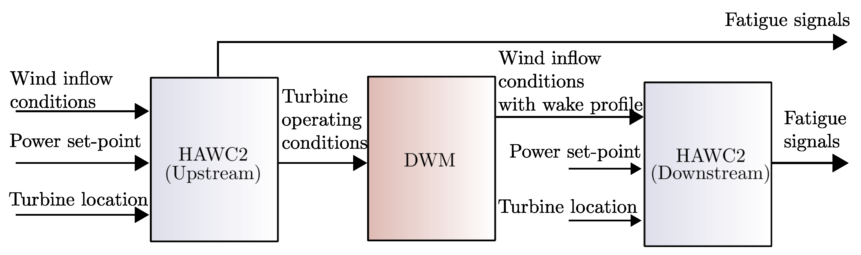
In this study, the HAWC2-DWM framework is utilised and a database is created, which serves as the basis for WT main component fatigue load prediction under various conditions in an array of turbines. Figure 2 depicts the HAWC2-DWM framework used in this work.
HAWC2 is an aeroelastic tool developed by the DTU Wind Energy Department and is used for the prediction of the wind turbine global response and loading under various external conditions.
The calculations are performed in the time domain, and Timoschenko beam elements are used for modelling the main structural parts of the turbine, such as the blades, the main shaft, the tower and the support structure. The turbine aerodynamics are captured with Blade Element Momentum (BEM) theory, including various corrections such as tip loss factor, dynamic inflow and dynamic stall effects. For the wake effects, the DWM model has been incorporated in the main code. The aerodynamic and wake model, in particular, has a long history of development and validation against experimental data—for both onshore and offshore applications [6,22,23].
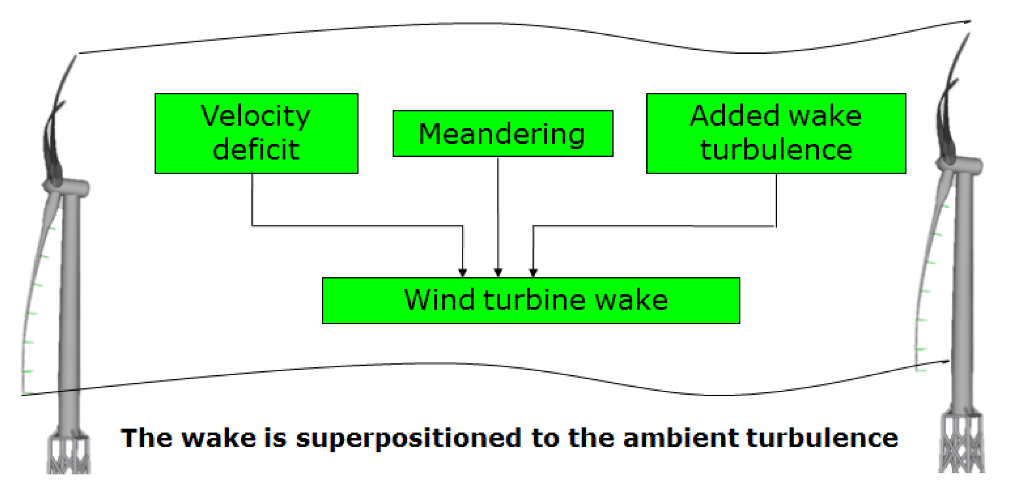
The DWM model captures the wakes generated by a wind turbine, where the wake is assumed to be transported downstream as a passive tracer by the large scale atmospheric turbulence structures. Three turbulence ‘boxes’ are used to model the overall change of the ambient turbulence based on the Mann model [24]. One large box with coarse grid size resolution (typically one rotor diameter) covers the entire wind farm and is used as the transport media of the wake deficits. The second turbulence box models the small eddies and micro-scale turbulence within the wake, and a third one covers the wind turbine rotor area for the ambient turbulence. The latter is the one that is also used in the simulations of stand alone wind turbines. The velocity deficit is extracted from the Blade Element Momentum (BEM) theory together with the boundary layer approximation of the Navier–Stokes equations. The DWM model takes into account the contribution of the strongest upstream WT wake up to rated (ambient) wind speeds, while summing linearly the upstream wakes for wind speeds above rated. As a result, for each turbine in a wind farm, the inflow wind field is a linear superposition of the ambient field, and any relevant wake deficit and induced small scale turbulence. Figure 3, which is taken from reference [18], illustrates how the wake effects are modelled.
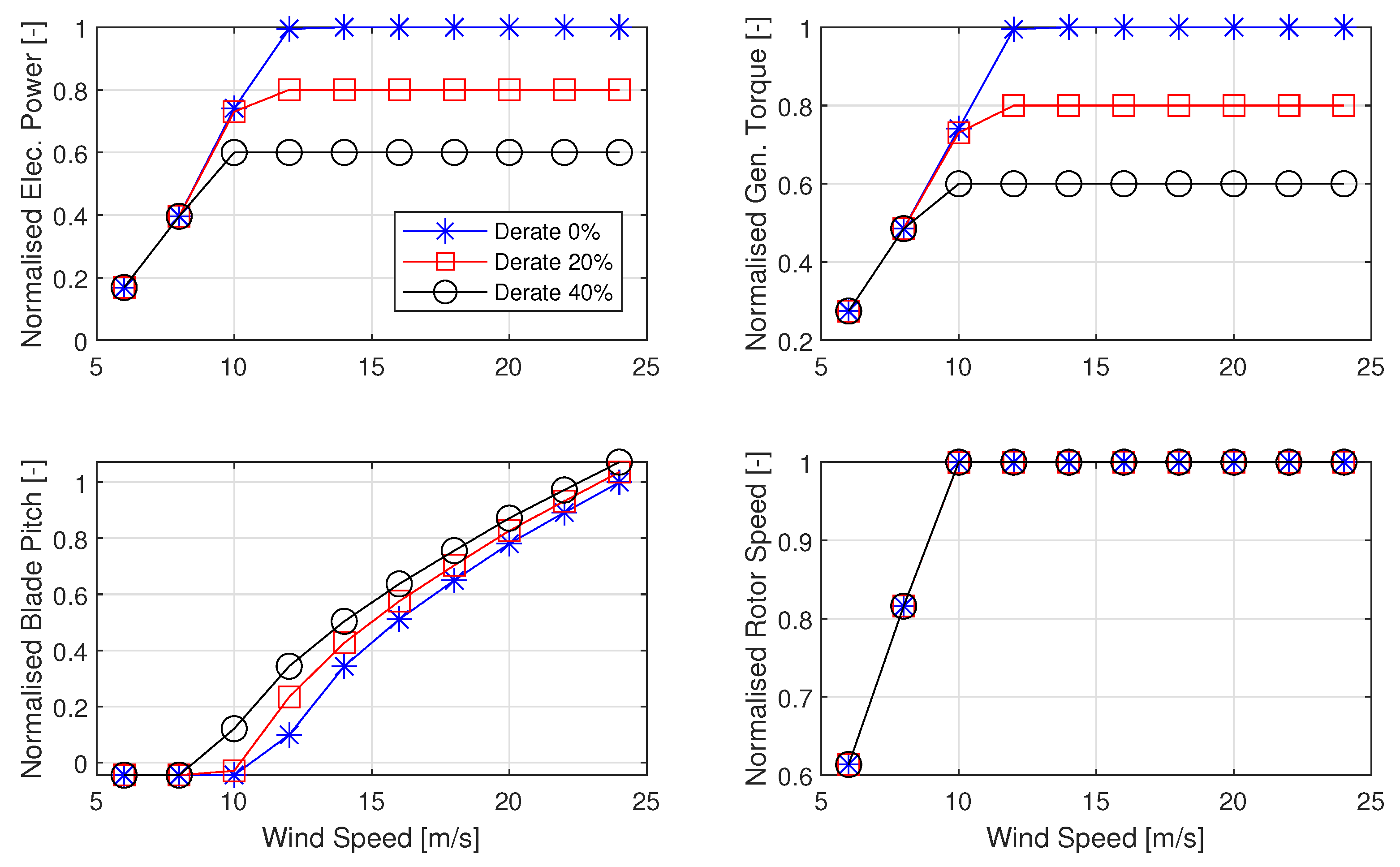
The input parameters for the current HAWC2-DWM implementation are the upstream turbine operational rotor speed and collective blade pitch angle for a given ambient inflow. This set of operating quasi-steady points alters the created deficit and turbulence mixing downstream, influencing the downstream turbine operation and loading. Down-regulation can be achieved by either changing the generator torque or pitch angle or both [25]. For this study, the maximum rotational speed (Max-) down-regulation is used, where the generator torque is modified as follows:
where is the power demand and is the rated rotor speed. The strategy ensures the rotor is operating at the maximum speed, thus reserving the kinetic spinning energy to support the power grid. As soon as the nominal rotor speed is reached, the blades are pitched towards feather to reduce the power to the desired level. This strategy is widely used in the literature (e.g. [26,27]). In Figure 4, the quasi-steady WT operational pitch angle and rotor speed, as well as the electrical power output and generator torque, are presented for different derating percentages. The results are normalised by the normal operation values at 24 m/s wind speed. The turbine controller increases the rotor speed as the wind speed increases until the nominal value, and then the pitch actuator turns the blade to feather in order to regulate the power.
2.4. Neural Network
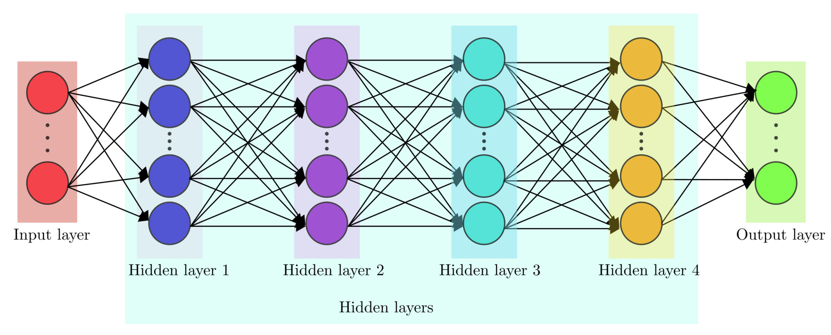
In this study, the T2FL model is constructed using artificial neural network (ANN) algorithms of MATLAB’s Neural Network Toolbox [28]. The choice was based on the fact that they are fast to train on a normal desktop computer. Furthermore, the fitting ANN type of function was selected with four hidden layers, which can fit any finite input–output mapping problem. It is expected that different algorithms will perform differently depending on the screened sensor type. More than one algorithm for each output is explored due to the fact of fast training of each algorithm and possible variations of their accuracy in the prediction. The fitting is done using the Bayesian Regularisation (BR) or the Levenberg–Marquardt (LM) algorithms. The BR algorithm minimises a linear combination of squared errors in the beginning and further modifies the linear combination in order for the ANN to have good global response [29]. The LM algorithm also known as the Damped Least-squares Method interpolates between the Gauss–Newton algorithm and the method of gradient descent. The LM is more robust compared to the Gauss–Newton algorithm. More about the LM algorithm can be found in [30,31]. Additionally, an ensemble of surrogate models is built and its performance is evaluated. An ensemble of surrogate models can reduce the tedious manual fine tuning work in the case of using one algorithm and can provide a more robust overall model. Figure 5 depicts the architecture of the artificial neural network with four layers used in this study.
Two metrics are used to evaluate the different algorithms. The first metric is the Root-Mean-Square Error (RMSE), which is defined in Equation (3), and the second metric is the Mean Absolute Error (MAE) at the evaluation points:
where N is the number of evaluation points and y, , are the actual and predicted outputs, respectively.
The MAE was also computed since each error contributes proportionally to the absolute value of the error. In contrast, the RMSE is characterised by the square of the error, and therefore weighs larger errors more. Lower metrics indicate better performance of the model predictions.
3. Verification of the Surrogate Model
Each model was trained using of the aeroelastic simulation results and the remaining for testing. Table 2 and Table 3 summarised the normalised RMSE and MAE metrics as evaluated based on the whole database. The values have been normalised by the actual simulated results of the upstream WT at 16 m/s wind speed and 7% turbulence intensity under normal power production. They represent how well the surrogate models are able to predict the loads and power at the same input parameters where aeroelastic simulations were performed. The results shown below have been normalised with the loads and power output of the turbine at 16 m/s wind speed. The individual algorithms had very similar metrics for the load evaluation, but for the power prediction, the BR metrics were around half of the LM ones. In other words, the BR algorithm performed better in the turbine power prediction. However, the ensemble of models outperformed both algorithms for all the sensors. It should be noted that a weighting factor of 0.5 was applied on the ensemble model creation of load outputs, since the error metrics between the BR and LM algorithms were similar. For the power, initially the weighing factors were set equal; however, due to the fact that the BR performed much better than the LM, a series of tests with increasing the BR weighting factor with a step of 0.1 were evaluated. A weighting factor of 0.8 for the BR and 0.2 for the LM algorithms was found by brute-force search to perform the best, and these results are reported in the tables.
4. Applications
4.1. Power and Fatigue Studies of Two-Turbine Wind Farms
It is very important to know the turbine component loads and the power output for every variation of the input parameters. The key results on wind farm power production and fatigue loads from the proposed surrogate model are presented and discussed through contour maps in Figure 6, Figure 7 and Figure 8.
4.1.1. Power Production
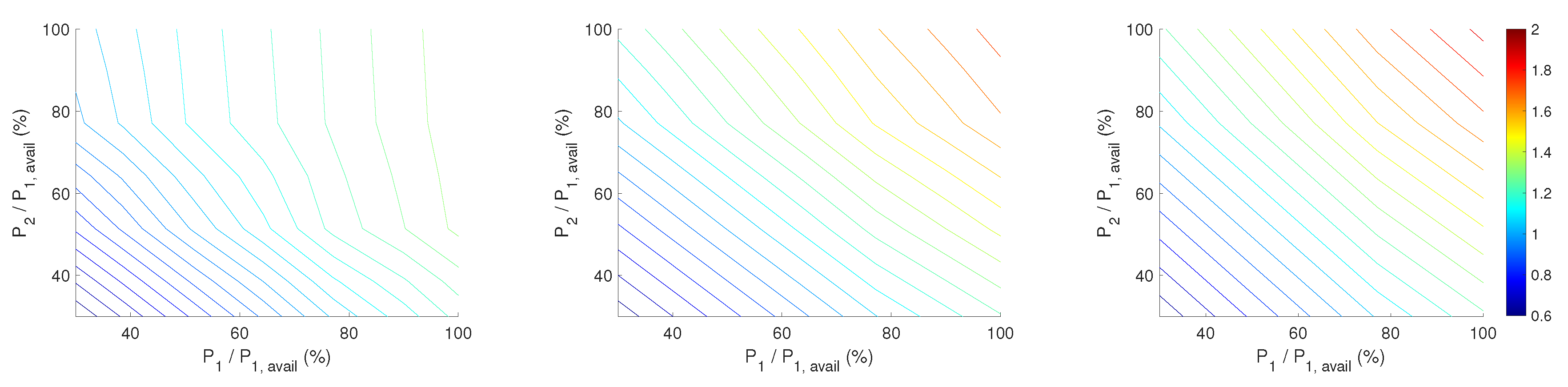
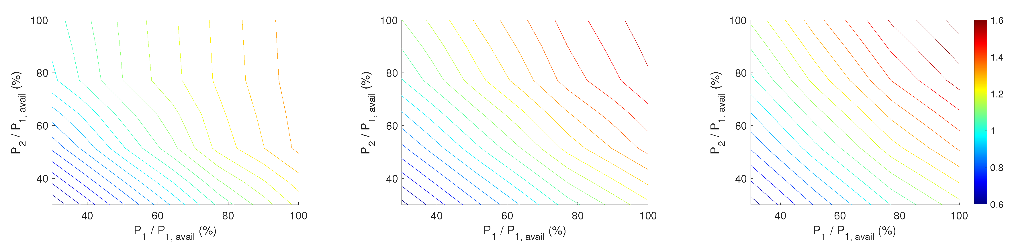
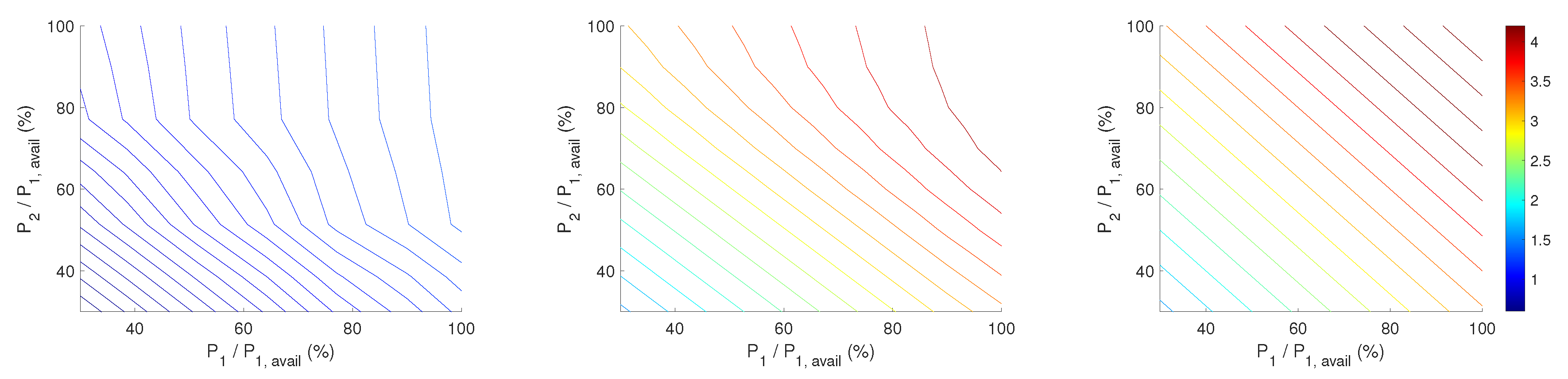
In Figure 6, Figure 7 and Figure 8, the normalised total power of the two turbine array is plotted as a function of WTs normalised power. The turbine array power normalisation is done with the available power of turbine one () at 8 m/s wind speed and 7% TI. Figure 6 presents results for three different incoming wind directions 0°, 10°, 22° from left to right plots at 8 m/s, 7% turbulence intensity and 5D turbine inter-spacing. In Figure 7 and Figure 8, the TI (7%, 14%, 27%) and wind speed (8, 12 and 16 m/s) were varied, respectively. The other parameters were kept the same. Figure 6, Figure 7 and Figure 8 reveal the total power gain by the wind farm by down-regulating turbine 1 and 2 under changes in wind direction, ambient turbulence intensity and mean wind speed, respectively. Figure 6 reveals the effect of wakes in power production because the wind direction affects the wake propagation. Moving from full wake (left plot) to no wake (right plot) effects, the array of turbines could produce more power for the same ambient wind speed and TI. An increase in the ambient TI also affected positively the turbine array power output, as seen in Figure 7. This is due to the higher mixing and eventually shorter wakes. Lastly, the most drastic effect in power, as expected, shown in Figure 8. At 16 m/s, the iso-contours are becoming straight lines, which means that the same power down regulation of either upstream or downstream WT would have the same effect on total power. This is because at 16 m/s, the downstream WT was able to produce the rated power, despite the wake effects of upstream. However, the component loads between the WTs were expected to be different and will be studied next.
4.1.2. Tower Fatigue Damage
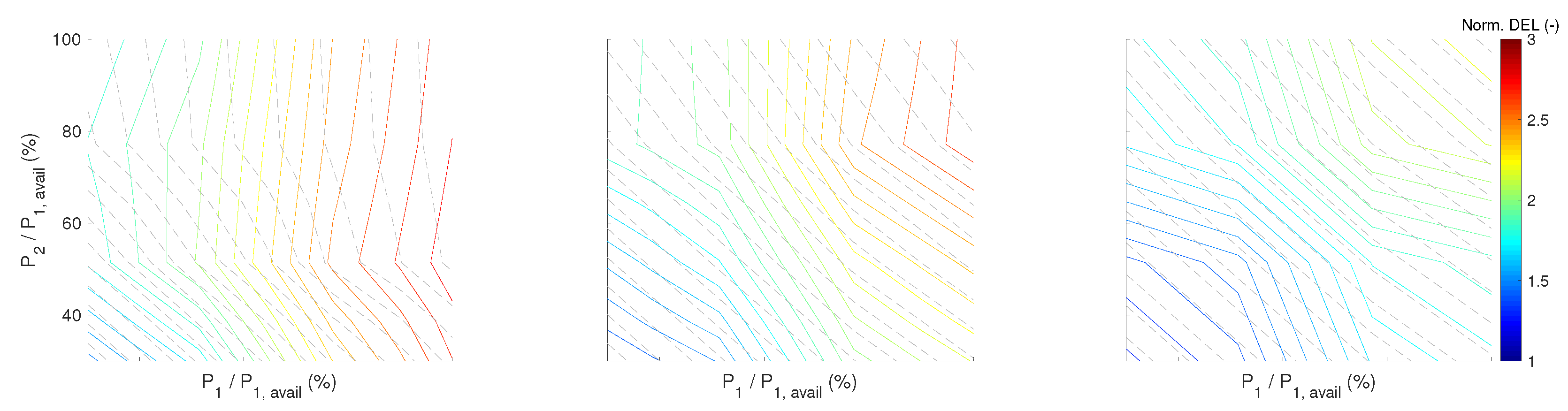
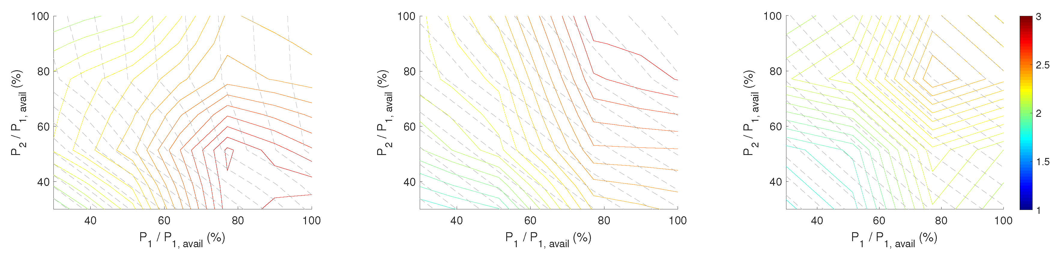
In Figure 9, Figure 10 and Figure 11, the sum of the normalised Tower Bottom Fore-Aft (TBFA) Damage Equivalent Loads (DEL) of the two turbine array are plotted with coloured contours as a function of WTs normalised power. The power normalisation is done with the available power of turbine one () at the given free wind speed. The grey dashed lines in the background denote contours of the same sum power output of the turbine array. These grey lines correspond to the plots of Figure 6, Figure 7 and Figure 8. In contrast, the fatigue load normalisation is done with the minimal total DEL of two turbines. Similar to Figure 6, Figure 9 presents results for three different incoming wind directions 0°, 10°, 22° from left to right plots at 8 m/s, 7% turbulence intensity and 5D turbine interspace. In Figure 10, the TI was varied (7%, 14%, 27%) from left to the right plots, while the other parameters were kept the same as in Figure 9. Similarly, Figure 11 shows results for different wind speeds (8, 12, 16 m/s) from left to right, while the other parameters were kept the same as in Figure 9.
Focusing on the left plot in Figure 9, it can be seen that the total normalised DEL was the highest for full power production of upstream turbine 1 () and letting downstream WT-2 produce as much as it could. As the wind direction changed from 0° to 10° and then 22° (centre and right plots), the total DEL decreased since the downstream WT was getting out of the wake of the upstream one. It can also be seen that for high curtailment operation of WT-1 and WT-2 (the lower left corner of the plot), the total tower DEL and total power output of the turbine array have a linear relation with very similar slope. As a result, the operation of each turbine could be regulated at a given total power setpoint such that each tower DEL could be redistributed among the turbines in order to reduce the imbalance of the lifetime fatigue between them. This linear behaviour and same slope between loads and power can also be seen for high curtailment operation at other wind conditions, as shown in Figure 10, centre and right plots, where the TI is 14% and 27%. The DEL was increasing with higher TI and wind speed, as observed in Figure 10 and Figure 11, respectively.
4.1.3. Blade Fatigue Damage
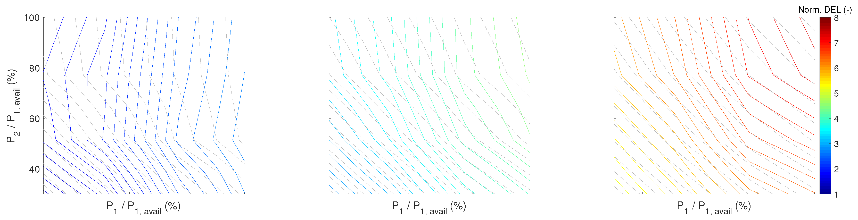
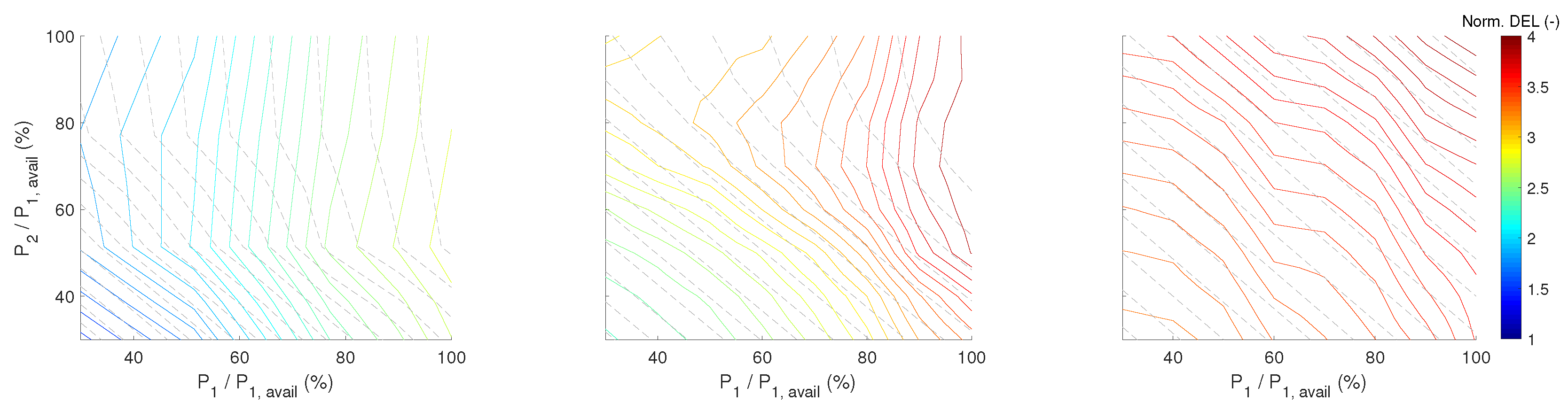
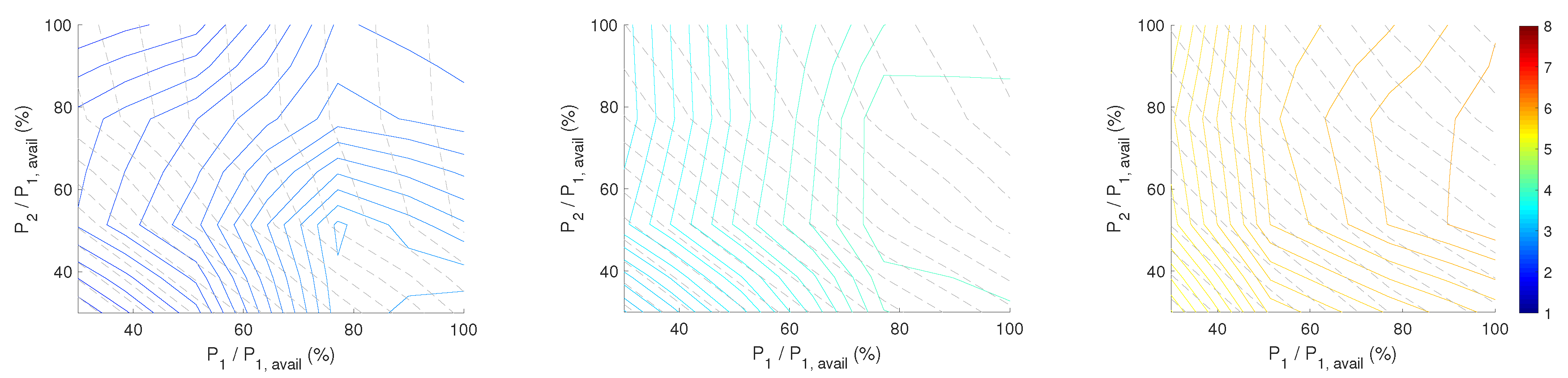
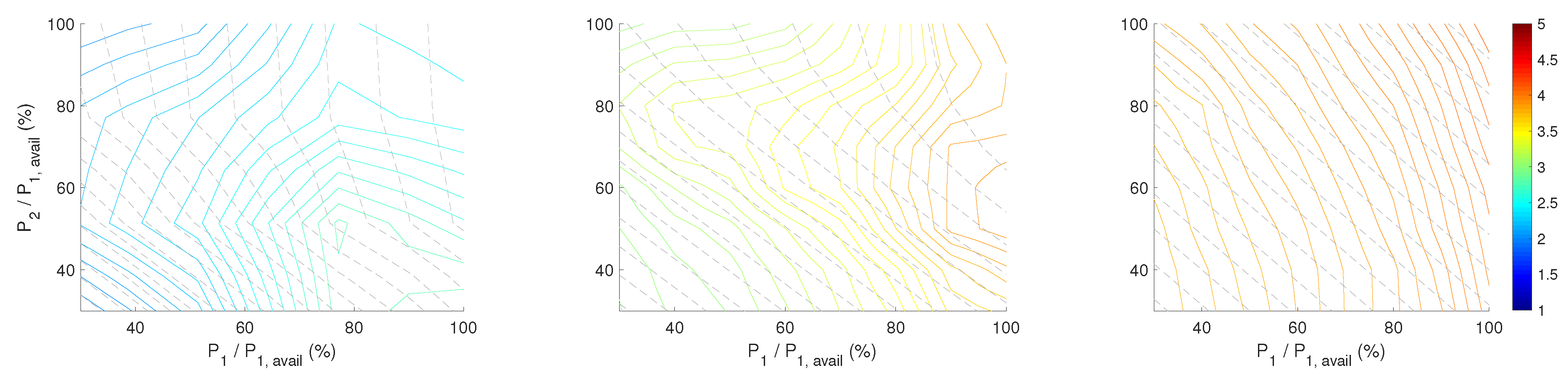
The blade root flapwise (BRF) DEL results for the same wind conditions and turbine interspace are presented in Figure 12, Figure 13 and Figure 14. Studying the left subplot of Figure 12, one can see that the total blade DEL had a similar pattern like the tower DEL at a high power de-rating of WT one and two and differs in the remaining area. For instance, it is possible to save on total blade fatigue when WT-1 is producing power of up to 80% and WT-2 is regulated above 60%. This can be seen by following the grey dashed constant turbine array power curves. For the partial wake and free wake situations, Figure 12 centre and right plots, the DEL contours had a similar pattern to the tower plots in Figure 9, Figure 10 and Figure 11. The effect of increasing turbulence is depicted in Figure 13, where TI increases from 7% to 14% and 27% from left to right. The tower loads and the blade loads increase a lot independently of the turbines operation set points, as the TI increased up to a factor of eight. The loads at different incoming wind speeds (8, 12, 16 m/s) were given in Figure 14. Operation of turbines at high wind speeds caused more total fatigue; however, it was still feasible to re-distribute the damage between the turbines.
The contour plots reveal that depending on the desired power output from the cluster of turbines, it is possible to minimise the total fatigue. Furthermore, it is also feasible to redistribute the fatigue loads between the WTs. For instance, at 14 m/s, 7% TI and 0 degrees wind direction and when the turbine array power is derated by 25% on available power, one can dig into the database and find more favourable operation points favourable more either for the upstream or the downstream turbine loads. In this specific case, the individual WT normalised TBFA loads can be between 1.632 to 1.3056 for the upstream, and 1.5154 to 1.9584 for the downstream, respectively. A systematic way of finding optimum WT operation set-points for a given power output, while minimising the loads, is presented in the next section.
4.2. Wind Farm Control: Synthesised Optimum Operation
The developed T2FL model can be used to estimate the individual turbine fatigue loads that emanate on various wind farm control strategies and for layout optimisation.
The T2FL model can be used in wind farm controllers to reduce fatigue loads during down-regulated wind farm operation. Typically such a control approach is realised using model-predictive control (MPC) [32,33]. The MPC objectives are to (i) follow the reference for the total power of the wind farm, (ii) reduce the fatigue loads of wind turbines, and potentially, (iii) other additional objectives. Hence, a typical objective function J can have the following form [34,35]
where is the reference for the total power of the wind farm at time step n, N is the number of steps of the prediction horizon of the MPC, is the power output of turbine i at time step n, I is the number of wind turbines in the wind farm. Function represents the objective of the wind farm operator with regards to turbine fatigue loads. As such, the operator could have the objective to minimise the sum fatigue loads of the wind farm, thus . is a weighting factor to trade off between the different parts of the objective function. The novel fatigue model T2FL provides the relation between power set-points of wind turbines and fatigue loads of wind turbines . Function shall represent any potential additional operational objectives. comprises the set-points of turbine power over the entire control horizon. The power set-point of a wind turbine is constrained by the available power of the wind turbine.
Example
The T2FL model can be used to derive operation strategies that optimise the fatigue-related objective of an operator. In the present study, the objective is the minimisation of the sum fatigue loads of wind turbine components in the wind farm. Such strategies could be derived manually, for instance from Figure 9, Figure 10 and Figure 11 for the tower. In the following, the optimum strategy is derived using numerical optimisation of the following problem
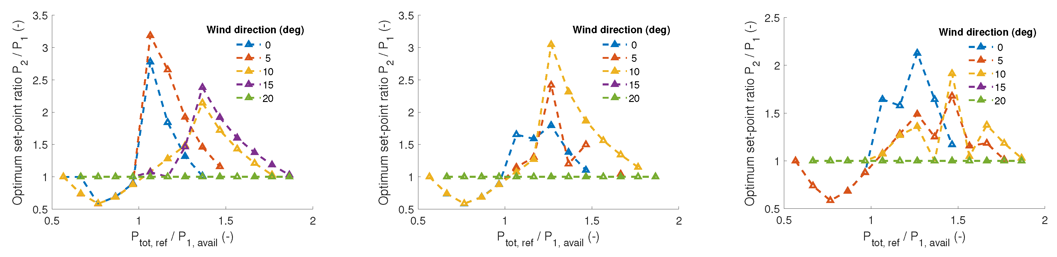
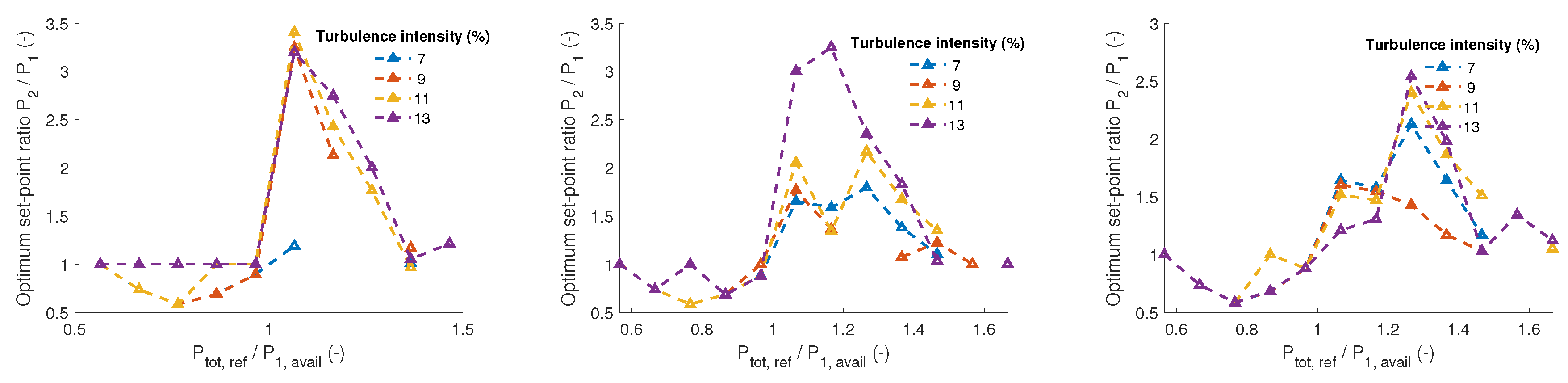
where are the power set-point of upstream turbine 1 and downstream turbine 2. is the reference for the mean total power output. are time-averaged power output of upstream turbine 1 and downstream turbine 2. Figure 15 and Figure 16 give the optimum ratios of turbine power set-points as a function of total power reference. The ambient wind is 8 m/s and going from left to right subplots, the turbine interspace is 5D, 7D and 9D, respectively. The wind direction is varied in Figure 15 from 0 to 20 degrees, while the turbulence intensity is varied from 7% to 13% in Figure 16. When the available power is insufficient to satisfy the demanded total reference power, the optimum strategy is nonexistent. This is the case in the plots where points do not exist for some combinations of power ratios. Focusing on the left plot in Figure 15, one can see that at 20 degrees wind direction, the optimum set-point ratio is constant for any ratio of . This is the case where the upstream WT wake does not affect the downstream WT wind field. For smaller wind direction angles, wake effects are present, and the optimum set-point varies. It is favourable for load minimisation to produce more power from the downstream WT rather than from the upstream one for ratios larger than 0.95, while the opposite is true for smaller ratios.
4.3. Wind Farm Layout Optimisation
The wind farm layout optimisation problem is inevitably part of every wind farm development project. After the selection of a suitable site and knowing the wind condition, the question arises of how many turbines should be installed and where. The objective typically is the maximisation of annual energy production, the minimisation of the Cost of Energy (COE) or their combination [36]. The COE can be split into the turbine installation, operation and maintenance and decommissioning. As such, the problem can include many sub-modules depending on the desired fidelity of the outcome. A multi-fidelity optimisation method for wind farms is given in paper [37]. The authors established three levels of complexity, with the third being the one with the highest fidelity. The approach was described, however was not implemented or considered in the optimisation loop. It considers turbine aeroelastic simulations coupled directly with the dynamic wake meandering model and would lead to the inclusion of the turbine component fatigue and remaining lifetime as the cost function. This is what the T2FL model can contribute to a WF layout optimisation framework, for example, TOPFARM [37]. The main WT component equivalent fatigue loads (, typically 1Hz) are given by the T2FL model. is a metric of how large the fatigue is and it is a way to compare arbitrary load time series by converting them to an equivalent value, which will have the same effect to the fatigue of the structure. Thus, it is possible to calculate the x-year lifetime fatigue damage () for any given wind conditions by Equation (7),
where the material dependent Wöhler exponent m and the x-year equivalent number of cycles are set to the desired values. T is the duration of each simulation in seconds and corresponds to equivalent cycles. is the probability of the mean wind speed U and is the number of simulations considered for each condition in order to capture the stochasticity of the wind turbulence taking into account the x-years of operation. Having as reference, one can compute the remaining lifetime of a component or the consumed one D by Equation (8).
where is the component accumulated fatigue damage and can also be calculated by Equation (7) knowing the fatigue loads for a given operation time interval.
5. Conclusions
An efficient wind farm load prediction framework has been presented in detail for the optimisation of turbine fatigue loads. It can be used for both wind farm layout optimisation and optimal control of wind farms. A case study of two turbines was demonstrated, and the wind farm controller set points were derived for minimisation of the sum fatigue loads within the farm. The study was based on high fidelity aeroelastic simulations, including the dynamic wake meandering model to account for the wake effects. A detailed analysis was given for the selection of the range of input parameters of the database. This is crucial since the number of parameters was large and directly affects the needed number of simulations.
A surrogate modelling approximation technique was introduced using artificial neural networks in order to minimise the number of simulated cases and to be able to predict the loads and power for a wide range of incoming wind conditions and turbine down regulation operations. Two algorithms were evaluated, the Bayesian Regularisation (BR), and the Levenberg–Marquardt (LM). Furthermore, an ensemble of the surrogate models was developed and evaluated. Results showed that the ensemble model outperformed both individual model predictions of the BR and LM algorithms. The case study of two turbines gave interesting insights into individual turbine loads and ways of distributing fatigue damage between turbines while optimising the power production. The result revealed that the minimal total fatigue load occurs when the downstream turbine produces more power than the upstream turbine. Additionally, the results revealed that it is possible to minimise overall fatigue damage during curtailed operation.
Author Contributions
The paper was a collaborative effort among the authors. C.G.: conceptualisation, methodology, Software, formal analysis, writing—original draft preparation, visualisation; J.K.: conceptualisation, writing—original draft preparation, investigation; W.H.L.: visualisation, writing—review and editing; G.G.: project administration, funding acquisition. All authors have read and agreed to the published version of the manuscript.
Funding
This work has been funded by the ForskEL Programme under project CONCERT—Control and unCERTainties in real-time power curves of offshore wind power plants (Grant No. 12396) and PowerKey—Enhanced WT control for Optimised WPP Operation (Grant No. 12558), and European Unions Horizon 2020 research programme under grant agreement no. 727680 (TotalControl).
Acknowledgments
The authors would also like to acknowledge Siemens Gamesa Renewable Energy for the provided wind turbine data.
Conflicts of Interest
The authors declare no conflict of interest.
References
- IEC. International Standard IEC61400-1: Wind Turbines-Part 1: Design Guidelines; IEC: Geneva, Switzerland, 2005. [Google Scholar]
- Frandsen, S. Turbulence and Turbulence Generated Fatigue in Wind Turbine Clusters; Technical Report Risø-R-1188; Risø National Laboratory: Roskilde, Denmark, 2007. [Google Scholar]
- Keck, R.E.; de Maré, M.; Churchfield, M.J.; Lee, S.; Larsen, G.; Madsen, H.A. Two improvements to the dynamic wake meandering model: Including the effects of atmospheric shear on wake turbulence and incorporating turbulence build-up in a row of wind turbines. Wind Energy 2013, 18, 111–132. [Google Scholar] [CrossRef]
- Larsen, G.C.; Madsen, H.A.; Thomsen, K.; Larsen, T.J. Wake meandering: A pragmatic approach. Wind Energy 2008, 11, 377–395. [Google Scholar] [CrossRef]
- Madsen, H.A.; Larsen, G.C.; Larsen, T.J.; Troldborg, N.; Mikkelsen, R.F. Calibration and Validation of the Dynamic Wake Meandering Model for Implementation in an Aeroelastic Code. J. Sol. Energy Eng. 2010, 132, 041014. [Google Scholar] [CrossRef]
- Larsen, T.J.; Madsen, H.A.; Larsen, G.C.; Hansen, K.S. Validation of the dynamic wake meander model for loads and power production in the Egmond aan Zee wind farm. Wind Energy 2013, 16, 605–624. [Google Scholar] [CrossRef] [Green Version]
- Galinos, C.; Dimitrov, N.; Larsen, T.J.; Natarajan, A.; Hansen, K.S. Mapping Wind Farm Loads and Power Production-A Case Study on Horns Rev 1. J. Phys. Conf. Ser. 2016, 753, 032010. [Google Scholar] [CrossRef]
- Dimitrov, N. Surrogate models for parameterized representation of wake-induced loads in wind farms. Wind Energy 2019, 22, 1371–1389. [Google Scholar] [CrossRef]
- Mendez Reyes, H.; Kanev, S.; Doekemeijer, B.; van Wingerden, J.W. Validation of a lookup-table approach to modeling turbine fatigue loads in wind farms under active wake control. Wind Energy Sci. Discuss. 2019, 4, 549–561. [Google Scholar] [CrossRef] [Green Version]
- Mirzaei, M.; Soltani, M.; Poulsen, N.; Niemann, H. Model based active power control of a wind turbine. In Proceedings of the American Control Conference, Portland, OR, USA, 4–6 June 2014; pp. 5037–5042. [Google Scholar] [CrossRef]
- Galinos, C.; Larsen, T.J.; Mirzaei, M. Impact on wind turbine loads from different down regulation control strategies. J. Phys. Conf. Ser. 2018, 1104, 012019. [Google Scholar] [CrossRef]
- Argyle, P.; Watson, S.; Montavon, C.; Jones, I.; Smith, M. Turbulence intensity within large offshore wind farms. In Proceedings of the European Wind Energy Association Annual Conference and Exhibition 2015, Ewea 2015-Scientific Proceedings, Paris, France, 10–12 March 2015; pp. 187–191. [Google Scholar]
- Göçmen, T.; Giebel, G. Estimation of turbulence intensity using rotor effective wind speed in Lillgrund and Horns Rev-I offshore wind farms. Renew. Energy 2016, 99, 524–532. [Google Scholar] [CrossRef] [Green Version]
- Ren, G.; Liu, J.; Wan, J.; Li, F.; Guo, Y.; Yu, D. The analysis of turbulence intensity based on wind speed data in onshore wind farms. Renew. Energy 2018, 123, 756–766. [Google Scholar] [CrossRef]
- Larsen, T.J.; Hansen, A.M. How to HAWC2, the User’s Manual; Technical Report R-1597(ver.12.7)(EN); Technical University of Denmark, Department of Wind Energy: Lyngby, Denmark, 2019. [Google Scholar]
- Matsuishi, M.; Endo, T. Fatigue of metals subjected to varying stress. Jpn. Soc. Mech. Eng. Fukuoka Jpn. 1968, 68, 37–40. [Google Scholar]
- Mirzaei, M.; Hansen, M.H.; Tibaldi, C.; Henriksen, L.C.; Hanis, T. Basic DTU Wind Energy Controller Version 2; Technical Report; Technical University of Denmark, Department of Wind Energy: Lyngby, Denmark, 2015. [Google Scholar]
- Larsen, T.; Larsen, G.; Aagaard Madsen, H.; Petersen, S. Wake effects above rated wind speed. An overlooked contributor to high loads in wind farms. In Proceedings of the Scientific Proceedings. EWEA Annual Conference and Exhibition 2015. European Wind Energy Association (EWEA), Paris, France, 10–12 March 2015; pp. 95–99. [Google Scholar]
- Wikipedia Contributors. Lillgrund Wind Farm—Wikipedia, The Free Encyclopedia. 2018. Available online: https://en.wikipedia.org/w/index.php?title=Lillgrund_Wind_Farm&oldid=867298522 (accessed on 21 August 2019).
- Available online: http://posspow.vindenergi.dtu.dk/ (accessed on 9 March 2020).
- IEC. International Standard IEC61400-3: Wind Turbines-Part 3: Design Requirements for Offshore Wind Turbines; IEC: Geneva, Switzerland, 2009. [Google Scholar]
- Larsen, T.J.; Larsen, G.C.; Madsen, H.A.; Thomsen, K.; Markkilde, P.S. Comparison of measured and simulated loads for the Siemens SWT 2.3 operating in wake conditions at the Lillgrund Wind Farm using HAWC2 and the dynamic wake meander model. In Proceedings of the EWEA Annual Conference and Exhibition, Paris, France, 17–20 November 2015. [Google Scholar]
- Madsen, H.A.; Sørensen, N.N.; Bak, C.; Troldborg, N.; Pirrung, G. Measured aerodynamic forces on a full scale 2MW turbine in comparison with EllipSys3D and HAWC2 simulations. J. Phys. Conf. Ser. 2018, 1037, 022011. [Google Scholar] [CrossRef]
- Mann, J. Wind Field Simulation. Probab. Eng. Mech. 1998, 13, 269–282. [Google Scholar] [CrossRef]
- Lio, W.H.; Mirzaei, M.; Larsen, G.C. On wind turbine down-regulation control strategies and rotor speed set-point. J. Phys. Conf. Ser. 2018, 1037, 032040. [Google Scholar] [CrossRef] [Green Version]
- Galinos, C.; Urbán, A.M.; Lio, W.H. Optimised de-rated wind turbine response and loading through extended controller gain-scheduling. J. Phys. Conf. Ser. 2019, 1222. [Google Scholar] [CrossRef]
- Lio, W.H.; Galinos, C.; Urban, A. Analysis and design of gain-scheduling blade-pitch controllers for wind turbine down-regulation. In Proceedings of the 15th IEEE International Conference on Control and Automation (IEEE ICCA 2019), Edinburgh, UK, 16–19 July 2019. [Google Scholar]
- MATLAB. Version 7.10.0 (R2018a); The MathWorks Inc.: Natick, MA, USA, 2019. [Google Scholar]
- MacKay, D.J. Bayesian interpolation. Neural Comput. 1992, 4, 415–447. [Google Scholar] [CrossRef]
- Marquardt, D.W. An algorithm for least-squares estimation of nonlinear parameters. J. Soc. Ind. Appl. Math. 1963, 11, 431–441. [Google Scholar] [CrossRef]
- Hagan, M.T.; Menhaj, M.B. Training feed forward networks with the marquardt algorithm. IEEE Trans. Neural Netw. 1994, 5, 989–993. [Google Scholar] [CrossRef]
- Kazda, J.; Merz, K.; Tande, J.O.; Cutululis, N.A. Mitigating Turbine Mechanical Loads Using Engineering Model Predictive Wind Farm Controller. J. Phys. Conf. Ser. 2018, 1104, 012036. [Google Scholar] [CrossRef] [Green Version]
- Kazda, J.; Cutululis, N. Model-optimised Dispatch for Closed-loop Power Control of Waked Wind Farms. IEEE Trans. Control Syst. Technol. 2019, 1–8. [Google Scholar] [CrossRef]
- Horvat, T.; Spudic, V.; Baotic, M. Quasi-stationary Optimal Control for Wind Farm with Closely Spaced Turbines. In Proceedings of the MIPRO, 35th International Convention, Opatija, Croatia, 21–25 May 2012; pp. 829–834. [Google Scholar]
- Soleimanzadeh, M.; Wisniewski, R.; Kanev, S. An Optimization Framework for Load and Power Distribution in Wind Farms. J. Wind Eng. Ind. Aerodyn. 2012, 107–108, 256–262. [Google Scholar] [CrossRef] [Green Version]
- Tesauro, A.; Réthoré, P.E.; Larsen, G.C. State of the art of wind farm optimization. In Proceedings of the Ewea 2012-European Wind Energy Conference and Exhibition, Copenhagen, Denmark, 16–19 April 2012. [Google Scholar]
- Available online: https://gitlab.windenergy.dtu.dk/TOPFARM/ (accessed on 9 March 2020).
Figure 1.
Illustration of the wind farm layout consisting of two turbines with diameter D and interspace l equal to x times the diameter.
Figure 1.
Illustration of the wind farm layout consisting of two turbines with diameter D and interspace l equal to x times the diameter.

Figure 2.
Illustration of the HAWC2-DWM framework for the prediction of turbine component fatigue damage.
Figure 2.
Illustration of the HAWC2-DWM framework for the prediction of turbine component fatigue damage.

Figure 3.
Illustration of the Dynamic Wake Meandering (DWM) method. The upfront wakes are superpositioned to the ambient turbulence, including a stochastic meandering process [18].
Figure 3.
Illustration of the Dynamic Wake Meandering (DWM) method. The upfront wakes are superpositioned to the ambient turbulence, including a stochastic meandering process [18].

Figure 4.
Normalised wind turbine mean electrical power, torque, blade pitch and rotor speed curves as a function of wind speed for different derating percentages.
Figure 4.
Normalised wind turbine mean electrical power, torque, blade pitch and rotor speed curves as a function of wind speed for different derating percentages.

Figure 5.
Schematics of the artificial neural network with four hidden layers.

Figure 6.
Contours of normalised power output of turbine array. Wind direction is 0, 10 and 22 degrees from left to right. Default wind conditions are mean wind speed of 8 m/s, turbulence intensity of 7%, and wind direction of 0 degrees, in which direction is aligned with turbine array. Turbine interspace is 5D.

Figure 7.
Contours of normalised power output of turbine array. Ambient turbulence intensity is 7%, 14% and 27% from left to right. Default wind conditions are mean wind speed of 8 m/s, turbulence intensity of 7%, and wind direction of 0 degrees, in which direction is aligned with turbine array. Turbine interspace is 5D.

Figure 8.
Contours of normalised power output of turbine array. Ambient mean wind speed is 8, 12 and 16 m/s from left to right. Default wind conditions are mean wind speed of 8 m/s, turbulence intensity of 7%, and wind direction of 0 degrees, in which direction is aligned with turbine array. Turbine interspace is 5D.

Figure 9.
Impact of wind conditions and turbine power set-points on simulated sum TBFA damage equivalent loads of two turbine array. Contour lines show sum TBFA loads normalised by the load of upstream turbine in default wind conditions. Grey dashed lines denote contours of same sum power output of turbine array. Wind direction is 0, 10 and 22 degrees from left to right. Default wind conditions are mean wind speed of 8 m/s, turbulence intensity of 7%, and wind direction of 0 degrees, in which direction is aligned with turbine array. The distance between the turbines is 5D.

Figure 10.
Impact of wind conditions and turbine power set-points on simulated sum Tower Bottom Fore-Aft (TBFA) damage equivalent loads of two turbine array. Contour lines show sum TBFA fatigue normalised loads. Ambient turbulence intensity is 7%, 14% and 27% from left to right.
Figure 10.
Impact of wind conditions and turbine power set-points on simulated sum Tower Bottom Fore-Aft (TBFA) damage equivalent loads of two turbine array. Contour lines show sum TBFA fatigue normalised loads. Ambient turbulence intensity is 7%, 14% and 27% from left to right.

Figure 11.
Impact of wind conditions and turbine power set-points on simulated sum TBFA damage equivalent loads of two turbine array. Contour lines show sum TBFA normalised fatigue loads. Ambient mean wind speed is 8, 12 and 16 m/s from left to right.
Figure 11.
Impact of wind conditions and turbine power set-points on simulated sum TBFA damage equivalent loads of two turbine array. Contour lines show sum TBFA normalised fatigue loads. Ambient mean wind speed is 8, 12 and 16 m/s from left to right.

Figure 12.
Impact of wind conditions and turbine power set-points on simulated sum blade root flapwise (BRF) damage equivalent loads of two turbine array. Contour lines show sum BRF fatigue loads normalised by the load of upstream turbine in default wind conditions. Grey dashed lines denote contours of same sum power output of turbine array. Wind direction is 0, 10 and 22 degrees from left to right. Default wind conditions are mean wind speed of 8 m/s, turbulence intensity of 7%, and wind direction of 0 degrees, in which direction is aligned with turbine array.

Figure 13.
Impact of wind conditions and turbine power set-points on simulated sum BRF damage equivalent loads of two turbine array. Contour lines show sum BRF normalised fatigue loads. Ambient turbulence intensity is 7%, 14% and 27% from left to right.
Figure 13.
Impact of wind conditions and turbine power set-points on simulated sum BRF damage equivalent loads of two turbine array. Contour lines show sum BRF normalised fatigue loads. Ambient turbulence intensity is 7%, 14% and 27% from left to right.

Figure 14.
Impact of wind conditions and turbine power set-points on simulated sum BRF damage equivalent loads of two turbine array. Contour lines show sum BRF normalised loads. Ambient mean wind speed is 8, 12 and 16 m/s from left to right.
Figure 14.
Impact of wind conditions and turbine power set-points on simulated sum BRF damage equivalent loads of two turbine array. Contour lines show sum BRF normalised loads. Ambient mean wind speed is 8, 12 and 16 m/s from left to right.

Figure 15.
Optimum ratios of turbine power set-points as a function of total power reference for different wind directions and turbine spacing. The ambient wind speed is 8 m/s, turbulence intensity is 7% and turbine spacing is 5D, 7D and 9D from left to right subplots.
Figure 15.
Optimum ratios of turbine power set-points as a function of total power reference for different wind directions and turbine spacing. The ambient wind speed is 8 m/s, turbulence intensity is 7% and turbine spacing is 5D, 7D and 9D from left to right subplots.

Figure 16.
Optimum ratios of turbine power set-points as a function of total power reference for different turbulence intensity (TI) and turbine spacing. The ambient wind speed is 8 m/s, wind direction is 0 degrees and turbine spacing is 5D, 7D and 9D from left to right subplots.
Figure 16.
Optimum ratios of turbine power set-points as a function of total power reference for different turbulence intensity (TI) and turbine spacing. The ambient wind speed is 8 m/s, wind direction is 0 degrees and turbine spacing is 5D, 7D and 9D from left to right subplots.


Table 1.
Summary of input variables, bounds and numbers of sampling points.
| Variable | Unit | Lower Bound | Upper Bound | Number of Sampling Point |
|---|---|---|---|---|
| (m/s) | 4 | 24 | 11 | |
| (deg) | 0 | 22 | 9 | |
| (%) | 7 | 27 | 3 | |
| (%) | 0 | 70 | 8 | |
| (%) | 0 | 70 | 8 | |
| l | (D) | 3 | 20 | 5 |
Table 2.
Normalised RMSE of the surrogate models.
| Model | Blade DEL (%) | Tower DEL (%) | El. Power (%) |
|---|---|---|---|
| BR | 1.145 | 1.253 | 0.029 |
| LM | 1.132 | 1.186 | 0.045 |
| Ensemble model | 1.054 | 1.118 | 0.028 |
Table 3.
Normalised MAE of the surrogate models.
| Model | Blade DEL (%) | Tower DEL (%) | El. Power (%) |
|---|---|---|---|
| BR | 0.753 | 0.829 | 0.015 |
| LM | 0.746 | 0.790 | 0.024 |
| Ensemble model | 0.680 | 0.732 | 0.015 |
© 2020 by the authors. Licensee MDPI, Basel, Switzerland. This article is an open access article distributed under the terms and conditions of the Creative Commons Attribution (CC BY) license (http://creativecommons.org/licenses/by/4.0/).
Share and Cite
MDPI and ACS Style
Galinos, C.; Kazda, J.; Lio, W.H.; Giebel, G. T2FL: An Efficient Model for Wind Turbine Fatigue Damage Prediction for the Two-Turbine Case. Energies 2020, 13, 1306. https://doi.org/10.3390/en13061306
AMA Style
Galinos C, Kazda J, Lio WH, Giebel G. T2FL: An Efficient Model for Wind Turbine Fatigue Damage Prediction for the Two-Turbine Case. Energies. 2020; 13(6):1306. https://doi.org/10.3390/en13061306
Chicago/Turabian StyleGalinos, Christos, Jonas Kazda, Wai Hou Lio, and Gregor Giebel. 2020. "T2FL: An Efficient Model for Wind Turbine Fatigue Damage Prediction for the Two-Turbine Case" Energies 13, no. 6: 1306. https://doi.org/10.3390/en13061306
Note that from the first issue of 2016, this journal uses article numbers instead of page numbers. See further details here.