An Optimal Air-Conditioner On-Off Control Scheme under Extremely Hot Weather Conditions

1
Qatar Environment and Energy Research Institute, Hamad Bin Khalifa University, Doha 5825, Qatar
2
ICube Laboratory, Université de Strasbourg-CNRS, 67000 Strasbourg, France
*
Author to whom correspondence should be addressed.
Energies 2020, 13(5), 1021; https://doi.org/10.3390/en13051021
Submission received: 24 December 2019
/
Revised: 12 February 2020
/
Accepted: 20 February 2020
/
Published: 25 February 2020
(This article belongs to the Special Issue Automation, Control and Energy Efficiency in Complex Systems)
Abstract
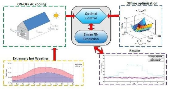
:Being reliant on Air Conditioning (AC) throughout the majority of the year, desert countries with extremely hot weather conditions such as Qatar are facing challenges in lowering weariness cost due to AC On-Off switching while maintaining an adequate level of comfort under a wide-range of ambient temperature variations. To address these challenges, this paper investigates an optimal On-Off control strategy to improve the AC utilization process. To overcome complexities of online optimization, a Elman Neural Networks (NN)-based estimator is proposed to estimate real values of the outdoor temperature, and make off-line optimization available. By looking up the optimum values solved from an off-line optimization scheme, the proposed control solutions can adaptively regulate the indoor temperature regardless of outdoor temperature variations. In addition, a cost function of multiple objectives, which consider both Coefficient of Performance (COP), and AC compressor weariness due to On-Off switching, is designed for the optimization target of minimum cost. Unlike conventional On-Off control methodologies, the proposed On-Off control technique can respond adaptively to match large-range (up to 20 C) ambient temperature variations while overcoming the drawbacks of long-time online optimization due to heavy computational load. Finally, the Elman NN based outdoor temperature estimator is validated with an acceptable accuracy and various validations for AC control optimization under Qatar’s real outdoor temperature conditions, which include three hot seasons, are conducted and analyzed. The results demonstrate the effectiveness and robustness of the proposed optimal On-Off control solution.
1. Introduction
Famous for its unique geographic location between desert and sea, Qatar has significant desert climate and extremely hot weather conditions with a high temperature, humidity, and sand storms. The Air Conditioning (AC) systems in this region are highly mandatory for daily life through the year. The local weather has some significance of representing a unique desert and coastline climate, which attract a lot of research interests in various fields such as building efficiency, health, urban environment, and renewable energy [1,2,3,4,5,6,7,8,9,10,11]. As elaborated in [12], in GCC region such as Saudi Arab, more than 60% of the electricity consumed by local buildings goes to Air conditioning (AC). This is particularly valid for other GCC countries like Qatar, which is reliant on AC throughout the majority of the year. Due to the persistent heavy cooling load caused by high temperature weather conditions and desert climate, heating, ventilation, and Air Conditioning (HVAC) equipment degrades faster compared to HVAC facilities in other areas and also requires higher reliability while maintaining energy efficiency and adequate levels of quality and comfort.
An Air Conditioner system is made up of a compressor as key part, and other parts such as a condenser and an evaporator, where the air conditioning capacity depends on the compressor power. In space cooling scenarios, indoor temperature will oscillate at a set-point because the compressor work in switch modes of on or off [13]. The component used to implement this control philosophy is known as an Air-Conditioner On-Off (or bang-bang) controller or thermoset. The On-Off compressor works as either being ON or OFF depending on the set-point boundary and the measured outdoor temperature. There is a dead range of 1.5 C to 2.0 C to prevent the too frequent On-Off fluctuations of the compressor that could lead to a reduced lifespan. Especially under hot weather conditions, long-term running with extra cooling load could degrade AC systems in a faster way, in particular if a very slight tracking error is imposed. Due to its simplicity, On-Off control is widely applied for temperature regulation application scenarios. However, On-Off control also have eminent drawbacks, which include temperature oscillation and non-optimal operation which negatively impacts the AC moving parts and its energy consumption [13,14,15,16,17,18,19,20,21].
Currently, a body of research work has been reported in the literature in response to challenges around HVAC control optimization. Several research works have been proposed to optimize building HVAC system [22,23], and address On-Off control issues under different constraints. The related research work can be summarized as two approaches: low-complexity optimization, and dynamic optimization. In low-complexity optimization approaches, Hysteresis controllers and Pulse Width Modulation (PWM) are widely utilized [13,24]. A hysteresis controller has a simple structure to implement in practice, so it is widely used in HVAC applications. Because the AC systems by hysteresis control work under fixed hysteresis conditions/parameters (with a set-point temperature boundary), the hysteresis controller does not perform well if ambient parameters/working conditions change. PWM control is usually used in PWM actuated split air conditioners. The PWM controller tunes the duty ratio of the AC On-Off control signal in a continuous way to allow continuous change of the manipulated variable. It can accommodate some work conditions change based on its fast feedback control, which is similar to Proportional-Integral-Derivative (PID) control. However, PWM controller has to change under very fast switching frequency at the initial stage of the control process or scenarios of large variations in the working conditions. This fast change could degrade the AC compressor, and it has also been proven not to be optimal for all the HVAC control cases. Both of these optimized controllers treat control process time horizon as a long-term general process in one day, one week, one month or one year. Thus, the full control process needs to rely on the temperature profile of an entire period and also the controller parameters can only be set and tuned in advance. For instance, the hysteresis control parameters are pre-set with a hysteresis result under certain working conditions. The controllers cannot accommodate ambient temperature variations in an adaptive way.
As a dynamic optimization approach, Model-Predictive Control (MPC) is employed to accommodate disturbances and variations of the operating conditions such as time-variant parameters and target [14,24,25,26,27,28,29,30,31]. The MPC’s optimization performance is subjected to the prediction horizon length. In theory, a longer prediction horizon can helps the solution be closer to the global optimum; therefore, it needs more computational power and resources. However, a proper prediction horizon is difficult to determine in practice, and MPC optimization will consume a lot of online computation loads. As such, online optimization and offline optimization need to be integrated and balanced for a trade-off between the computational load and AC control adaptiveness. In [32], a scheme of AC On-Off control and optimization is proposed for variant ambient conditions, but the transition between off-line optimization and online control is not integrated, and the part of outdoor temperature prediction is missing because it is assumed. Moreover, demonstrations under Qatar climatic conditions for three hot seasons of a full year are missing.
Motivated by the heavy cooling demand and its associated HVAC components wearing issues under harsh weather conditions in desert countries such as Qatar, an optimal AC On-Off Control Scheme is presented to improve cooling performance under heavy cooling load scenarios. In this scheme, optimizations are performed offline to generate the optimal solutions under certain conditions and range of outdoor temperatures, and then, a static data table of optimized parameters is generated. Based on the proposed lookup algorithm for online optimization, On-Off control parameters are tuned online to accommodate outdoor temperatures variation. As opposed to the existing AC hysteresis On-Off control schemes, the proposed On-Off control and optimization scheme can process more complex cooling scenarios such as large range and fast temperature variations. This is because the controller can adaptively accommodate the variations by tuning the parameters optimization online. Compared to the MPC control, the proposed control scheme performs optimization work offline which does not require a huge computational power in a real-time way like the online optimization technique.
This paper is structured as follows: a typical Qatar outdoor temperature profile is analyzed and the thermal model of a simple house is built in Section 2; Section 3 presents the proposed optimal On-Off control scheme, which includes off-line optimization and online adaptive tracking scheme. The validation results under different cooling scenarios are presented in Section 4 and Section 5 concludes the paper.
2. Problem Formulation
Due to Qatar’s unique geographical environment, the outdoor environment shows a very unique desert climate with high temperature. According to the data from local weather records shown in Figure 1, the average outdoor temperature varies from 15 C to 46 C throughout the four seasons. The daily temperature variation range could be up to 20 C during autumn or spring. This makes it necessary to study a typical thermal dynamics of a house with the local outdoor temperature profile analysis.
2.1. Outdoor Temperature Measurement under Qatar Weather Conditions
A three-day outdoor temperature profile in October 2017, which represents typical weather characteristics of Qatar, is measured in real time using thermal sensors at the outdoor test facilities of Qatar Environment and Energy Research Institute (QEERI). The facilities are shown in Figure 2, and the three-day profile is shown in Figure 3. The outdoor facilities site mainly host renewable energy facilities such as 200 kW PV farm, 250 kW/500 kWh Lithium-ion battery storage system, and other micro-grid components. Moreover, a weather measurement station for solar irradiance and other weather parameters, which include the outdoor temperatures, is deployed for research purposes. The daily outdoor temperature variations in October, shown in Figure 3, have a very uniform probability distribution, which means that the weather prediction can be performed with higher accuracy. In practice, one day ahead prediction horizon is available for outdoor temperature prediction based on existing weather measurement and prediction technologies. Thus, it is feasible to have enough time to do offline optimization in advance based on predicted weather conditions, which can prevent the complexities of online optimization.
2.2. House Thermal Model
To mimic thermal dynamics of a house, an Air-Conditioned house with heat exchange diagram is shown in Figure 4 [32]. The model thermal dynamics related equations can be denoted as follows:
By combining Equations (1) and (2), the house thermal dynamics are derived as follows:
The parameters in the above equations are defined in reference to the Table 1 of [32]. For simplicity, several assumptions need to be clarified to formulate the HVAC control problem. These assumptions are
- The AC system works only in cooling mode, which removes heat from the room;
- The AC house is modelled as a first-order state-space physical system;
- Only heat transferred from the outdoors is considered;
Remark 1.
The assumption of only cooling mode fits Qatar’s weather conditions because for most of the year (three hot seasons), the daytime outdoor temperature is over 25 C, and only AC cooling is needed. The last two assumptions are general for AC control and optimization studies, but it could be different in parameter setting for representing various application scenarios. For example, the indicator for extremely hot weather outdoor temperatures are considered as be time-variant in the studied house model.
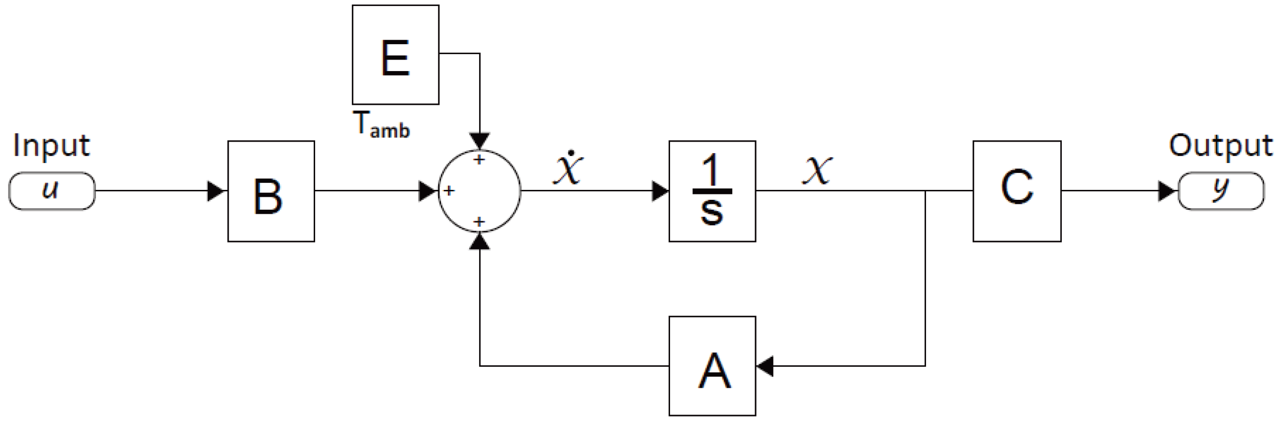
Based on the assumptions mentioned above, the house thermal model can be reformulated as a state-space model structure shown in Figure 5.
The mathematical format of the state-space model shown in Figure 5 can be represented as follows:
In Equation (4), the variables and parameters have the following physical meaning: x is the vector of the state, is the corresponding time derivative, u and y is the input vector and the output vector, respectively, A,B,C, and E is the corresponding state-space coefficient matrixes. Of note, x represents the state , which is measurable, and therefore . If denotes the rated power consumed by AC when the status is ON, u represents the On-Off control input , and it holds:
By converting Equation (3) into the format of equations (4), the coefficients A,B,E can be expressed as follows:
Remark 2.
In Equations (6), the term E is a function of , which means that if is changes as a variable and is not constant, the state-space model of Equation (4) could be more complex. Because the dynamics in (4) will be changed as first-order state-space model with time-variant parameters. Therefore, the control input (shows in u) needs to adaptively accommodate the disturbance E due to time-varying outdoor temperature. Moreover, with a full consideration on both comfort level and On-Off switch weariness, multiple optimizations are needed to improve the control strategy to achieve an optimal solution for multiple objectives.
3. Optimal On-Off Control for Time-Variant Outdoor Temperature
In this section, an optimal AC On-off control methodology is presented for stabilizing the room temperature regardless of the outdoor temperature variations. The optimal control scheme can be divided into an offline phase and an online phase. The offline phase is to solve optimum solutions by corresponding solvers for multiple objectives, while the online phase is to regulate the indoor temperature by tuning the controller with the updated parameters from the offline optimization.
3.1. Offline Multiple-Objective Optimization
3.1.1. Dynamics Subjected to On-Off Control
Because the control variable u in Equation (4) indicates On-Off binary variables, the solution of Equation (4) is different from the analytical solution of the standard state-space equation. The time-domain analytical solution can be written as follows:
Figure 6 presents the physical meanings of the variables and parameters in by a diagram of oscillation period dynamics. Based on the temporal relationship shown in Figure 6, the following mathematics must hold:
In addition, and can be derived from Equation (7) under , , and . The solution is shown as follows:
3.1.2. Cost Function for Multiple-Objective Optimization
Considering lowering the weariness cost due to AC On-Off switching while maintaining an adequate level of comfort in Coefficient of Performance (COP) value, the cost function can be defined as follows:
where J denotes the cost of one period of oscillation in one cycle and denotes the switching cost leading to weariness and is assumed to be constant. Q and R denote the weight coefficients of the COP cost and the switching cost. is the target indoor temperature. To convert this optimization as a convex optimization problem, the optimization variables of , can be converted into T and , their boundary conditions holds:
The optimization process leads to the following optimal solution:
3.1.3. Optimization Result Lookup Table Generation
With the proposed cost function in (10) constrained by the boundary conditions in (11), an offline optimization algorithm is designed to generate the optimum parameters for online adaptive On-Off Control. The flow chart of the offline optimization is shown in Figure 7, and the details can be referred in the justification of Figure 3 in [32].
3.2. Online Adaptive Control for Variable Outdoor Temperature
By looking up the optimum parameters generated by offline optimizations, the online control scheme can adaptively accommodate outdoor temperature variations with a light computational load. The online control scheme is comprised of three parts: outdoor temperature profile discretion, online adaptive control, and Outdoor temperature prediction.
3.2.1. Temperature Profile Discretion
Normally, the outdoor temperature is recorded by one-hour intervals. However, if we analyze the temperature profile of Qatar, it shows slow variation properties. Thus, variation within one hour is not notable. Moreover, it is not necessary to use hourly outdoor weather data because more hour points in a day means more duplicate or similar optimization procedures are needed. Therefore, to simplify the proposed online control scheme, the one-hour temperature profile needs to be discretized as longer intervals such as 2-h interval or 4-h interval. To implement the discretion, some interpolation algorithms such as nearest neighbor interpolation and linear interpolation can be applied, Interpolation results for the example of a 3-day profile with different intervals are shown in Figure 8.
3.2.2. Online Adaptive Control Scheme
After the outdoor temperature profile is discretized, the online adaptive control scheme is employed to stabilize the indoor temperature and accommodate the temperature variations adaptively. Figure 9 shows a flowchart of the proposed online AC control scheme. Firstly, the normal On-Off control is initiated to enable the AC system to converge into the target temperature range. Secondly, two cascaded control loops are executed. The outer control loop works to tune the On-Off controller parameters with the optimized solution. The inner loop works on the search for optimum parameter set by the index in a lookup table, which is previously generated online, in one horizon period. Finally, the scheme ends if all the time horizon of a full day is scanned.
3.2.3. Outdoor Temperature Prediction
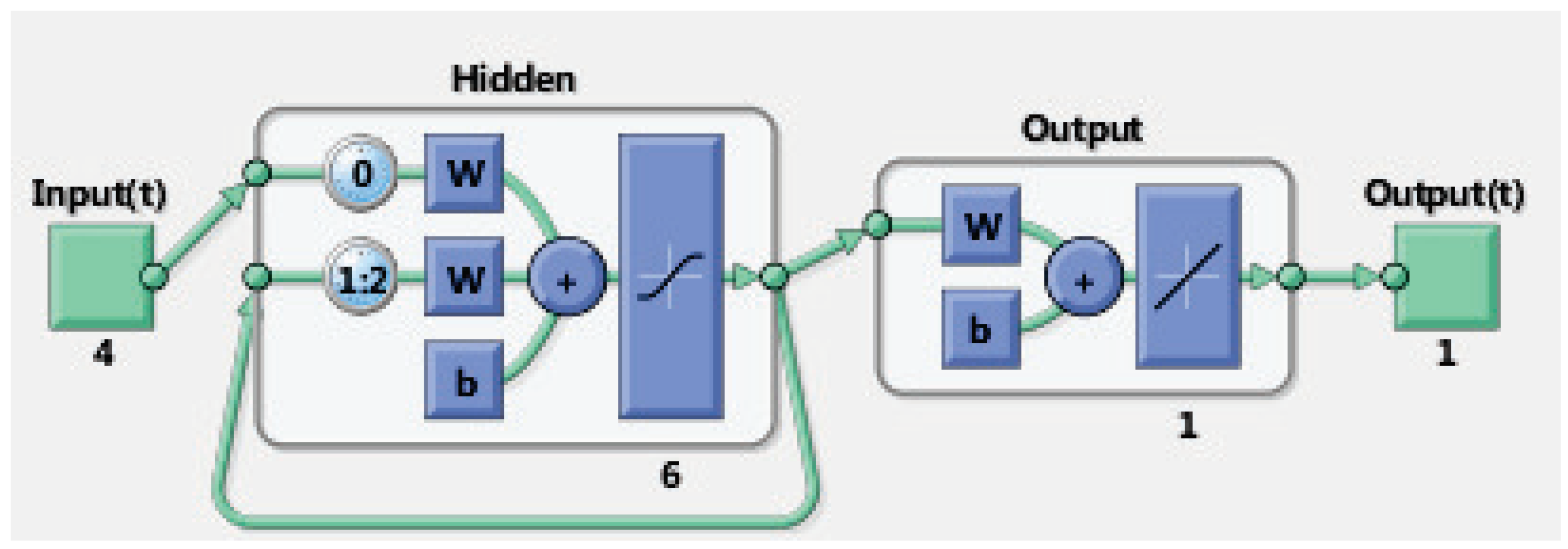
Temperature prediction is important for AC optimization control because the optimization objectives cover a period of control step processes. In the studied optimal control scenarios, at least 2 h ahead, prediction is mandatory for the online control process. With the consideration on a trade-off between prediction accuracy and computational complexities, a typical Elman Neural Network (NN) model shown in Figure 10 is employed as an estimator for outdoor temperature prediction.
To represent the prediction process, the outdoor temperature series can be denoted as follows:
Due to the temporal relativity of the outdoor temperature in the time domain, the outdoor temperature variation process can be denoted as follows:
where denotes the outdoor temperature at current instant k, is the function between and the temperature series at previous instants . For temperature time series prediction, a mapping model is needed to build firstly for approximating the mapping function . In this paper, a two-layer (second order) Elman neural network model in Figure 10 is proposed to approximate the mapping function . The mathematical representation of Elman network can be denoted as follows:
where , , are weight coefficients, , are offset coefficients, and are activation functions for hidden layer output and output layer respectively. For the outdoor temperature prediction, different prediction windows configurations exist. Depending on the availability of data series length, the input data vector length M could be 2, 3, …, 24. Thus, the cascaded prediction equations can be represented as follows:
Here, denotes the predicted or estimated value by the Elman NN model, denotes the prediction step number based on M existing temperature serial data. To get an effective and high-accuracy estimation model, the Elman NN offline training based on a set of sample data is essential and needs to be done in advance. Thus, the training problems of the Elman NN can be denoted as follows: Given a set of sample dataset as
By selected training algorithms, the Elman NN model parameters such as , , and weight coefficients, , can be determined based on the following criteria:
4. Validation Results
To validate the proposed On-Off control and optimization scheme, the studied house model parameters are referred from [13], and the AC power is changed as 1500 W but not 300 W because It is more reasonable due to the hot climate in Qatar. Moreover, to the best of our knowledge, the HVAC facilities in Qatar is prone to easily degrading and failing and normally need a high maintenance cost. Considering the fact that the AC weariness under hot climate is more serious, the weight factors of Q in (10) are reduced to reflect the factor of cost impact. The updated parameters are shown in Table 1.
Based on the AC parameter model list in Table 1, the proposed control and optimization scheme is demonstrated, which includes offline optimization and online AC control performance, in different cooling scenarios.
4.1. Offline Optimization Results
To verify the offline optimization performance, a simplified AC cooling scenario is assumed for comparison in a quantitative way. In this cooling scenario, the indoor temperature is expected to be 24 C by different controller parameter settings with the outdoor temperature set as 34 C. For comparison, the temperature profiles subjected to three types of controller settings are shown in Figure 11, and the corresponding COP values are compared. Figure 11 shows that the COP value of the proposed optimum control is the lowest at among optimization and non-optimization scenarios. Based on the cost value comparison, the optimum case has lower cost value, which means that it achieves better multiple-objective optimizations than other control scenarios. The cost-saving performance among the three cooling scenarios are presented in Table 2. As shown in Table 2, 30.16% can be saved from the case under outdoor temperature 29 C while 55.45% can be saved from the case under outdoor temperature 38 C by comparing with the optimum case.
To verify the effectiveness of offline optimization under different ambient temperature scenarios, a set of offline optimizations subjected to outdoor temperature range between 30 C and 44 C was performed. The target indoor temperature is expected to 24 C. The offline optimization parameters are shown in Table 3, and the optimization convex surface results are shown in Figure 12, which presents eight subfigures for eight temperature profiles with 2 C intervals. As can be seen from Figure 12, all the optimization surfaces are convex, which means that the global optimum solution for the studied optimization case exists and only one solution exists and is unique. Due to the impact of the ambient temperature, the optimization surface shapes and cost values vary in a large range. As an input for the online adaptive control, the corresponding optimization control parameters are also generated in a list of a lookup table.
4.2. Outdoor Temperature Prediction Results
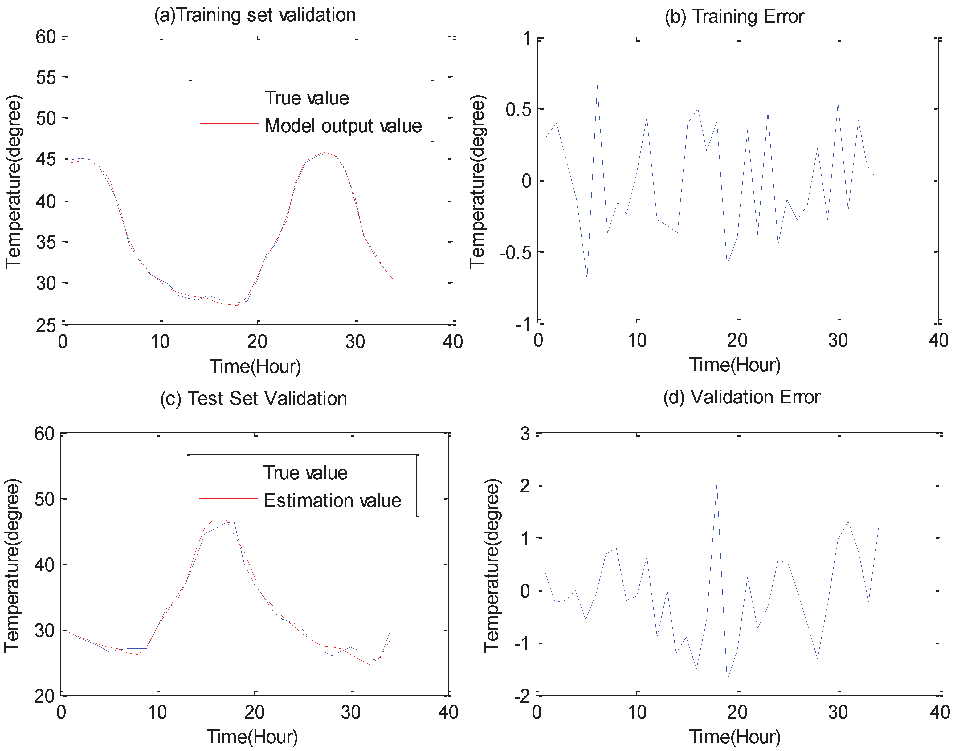
To validate the effectiveness of the proposed Elman NN based outdoor temperature prediction, the 3-day outdoor profile shown in Figure 3 was used for Elman NN model training and test. The 3-day temperature has 72 points of hourly temperature in total. The prediction window is set as 4 so the total data point number for NN test set is , and it is divided into two groups, 34 points each. After selecting the proper values for the Elman Training algorithm, we can get the training results in Figure 13a,b. From Figure 13a we can see that the Elman model output value is very close to the true value by the training procedure regression. From Figure 13b we can see that the error is less than 0.6 degrees, which means the model regression accuracy is very high. To test the generalization ability of the proposed Elman NN model, the other group of 34 points data is used for validation, and the results are shown in Figure 13c,d. From Figure 13c, we can see that the estimation value is also very close to the true value. From Figure 13d we can see that the estimation error is within the acceptable range (less than 2 degrees) although it is a little higher than training error. Based on the training regression and test validation results, we can conclude that the Elman NN model can generate an effective prediction of outdoor temperatures.
4.3. Online Adaptive Control Results
To validate the proposed online adaptive control scheme for the AC cooling under Qatar weather conditions, daily indoor temperature control scenarios are considered in the this paper. In general, the comfort indoor temperature is set as 25 C with an acceptable variation range of 2 C. Moreover, due to the slow time-variant characteristics of the outdoor temperature, a two-hour interval is a reasonable time zone to evaluate the weather temperature in existing weather measurement applications.
4.3.1. Case 1- One-Day Typical Case in Doha of Qatar
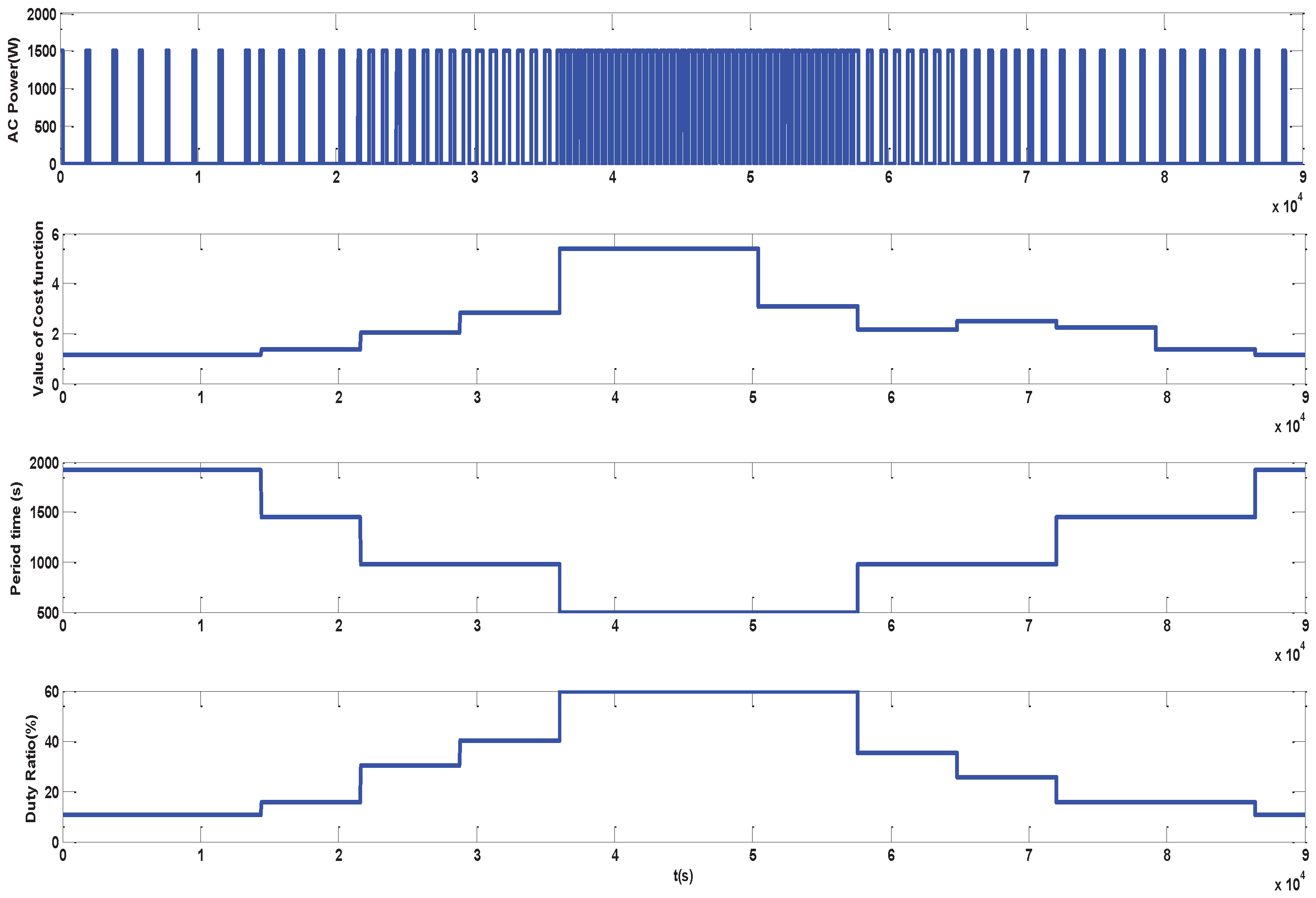
To verify the effectiveness of the proposed scheme, the second day outdoor temperature profile in Figure 3, which is a typical day with large temperature variations, was selected for the data analysis. To compare the performance between the proposed optimal control and the PWM control mentioned in the literature review, comparative experiments are also conducted to re-implement the PWM control in the same house model as the proposed optimal control under same Qatar outdoor condition. The implemented PWM control has an adjustable pulse-width based PID control structure. In this PWM control, the PWM period is constant while the duty ratio/pulse width is adjusted as a continuous control variable to avoid the fast switching in the On-Off control. In addition, a PID module is added to make the tracking control to converge in a smooth way with acceptable oscillation error. The PWM control diagram is shown in Figure 14, and the period time of the PWM pulse is set as 500 s, which is similar as the minimum period of the optimal control. The detailed AC control process variables such as AC consumption power, period time and duty ratio are shown in Figure 15, and the temperature control results are presented in Figure 16.
Figure 15 shows a modulated pulse output of the AC control power, cost value, period time, and duty ratios respectively. As can be seen from the plot of the AC power output, the AC consumption power is fixed at rated 1500 W while the pulse width is variable due to different cooling loads. The cost value plot also changes with time and shows a peak when the corresponding pulse width is the shortest. This means that a high outdoor temperature generates a heavier cooling load and more frequent AC On-Off switching actions and thus, the AC cooling overall cost is higher. From the period plot, we can see that the period time shows a valley point which it corresponds the closet pulse. From the duty ratio plot we can see that the duty ratio also reaches a peak point when the heavy load is highest. In a summary of all the plots, the results demonstrate that the control process can track the ambient temperature change and respond with appropriate control action in a real-time manner.
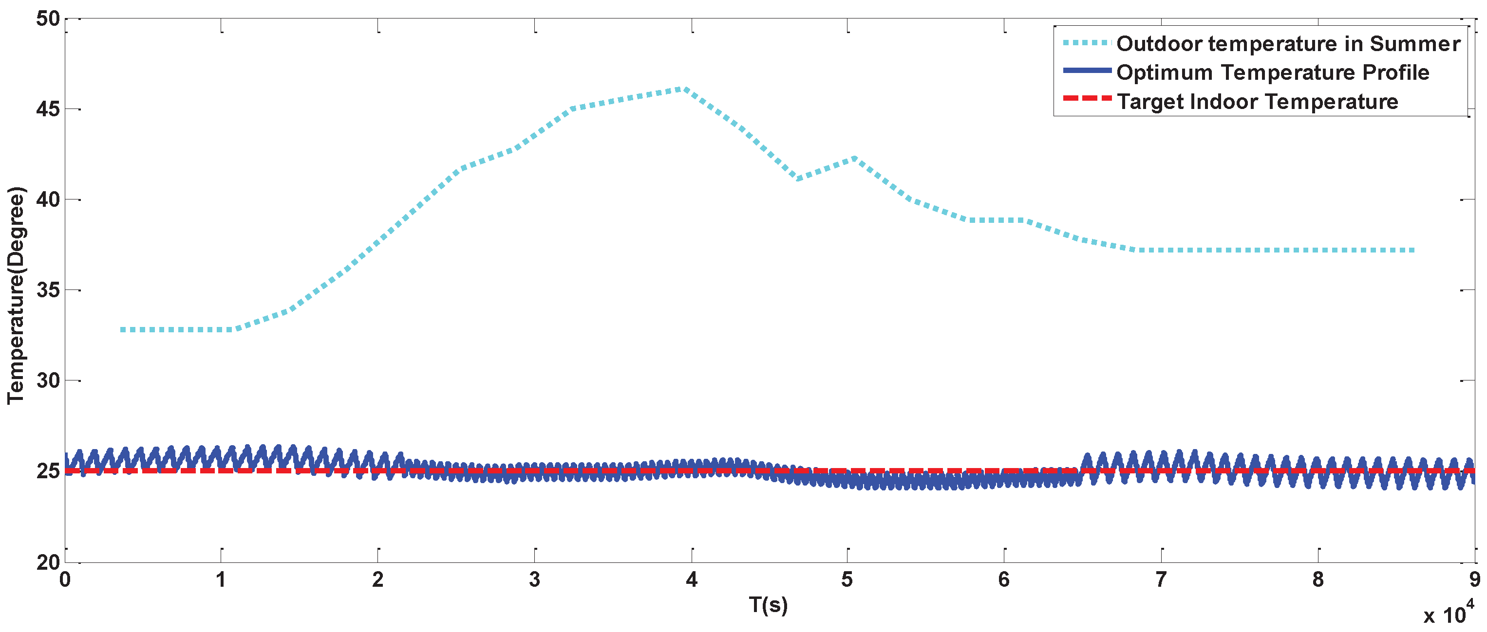
Figure 16 shows that the optimization AC cooling results under a typical day in summer. From the indoor temperature profile, we can see that the control scheme is effective to stabilize the indoor temperature at 25 C and be within the temperature fluctuation range although the curve is a little offset from the target curve at some instances. From the outdoor temperature profile, we can see that the outdoor temperature changes from 27 C to 46 C at a gap almost 20 C, but the control process can adaptively accommodate these variations by adjusting the control optimization parameters. Therefore, it is demonstrated that the proposed scheme applies for a typical large-variation scenario.
In addition, Figure 16 also shows the temperature profile comparison between the PWM control and the proposed optimal control. Both the PWM control and the optimal control can stabilize the target indoor temperature at 25 C, although the outdoor temperature changes in a large daily range of 20 C. The PWM control oscillates at the transition time of the outdoor temperature’s rapid change while the proposed optimal control can accommodate this rapid transition in a smoother way. Moreover, the rapid transition causes the PWM control taking a large range of oscillation (between 23 C to 27 C) to converge into the target indoor temperature 25 C, while the optimal control can stabilize at a smaller range (between 24 C to 26 C). Through this comparison, it can be demonstrated that the optimal control has a better control performance than the PWM control in both stabilization accuracy and transition convergence speed.
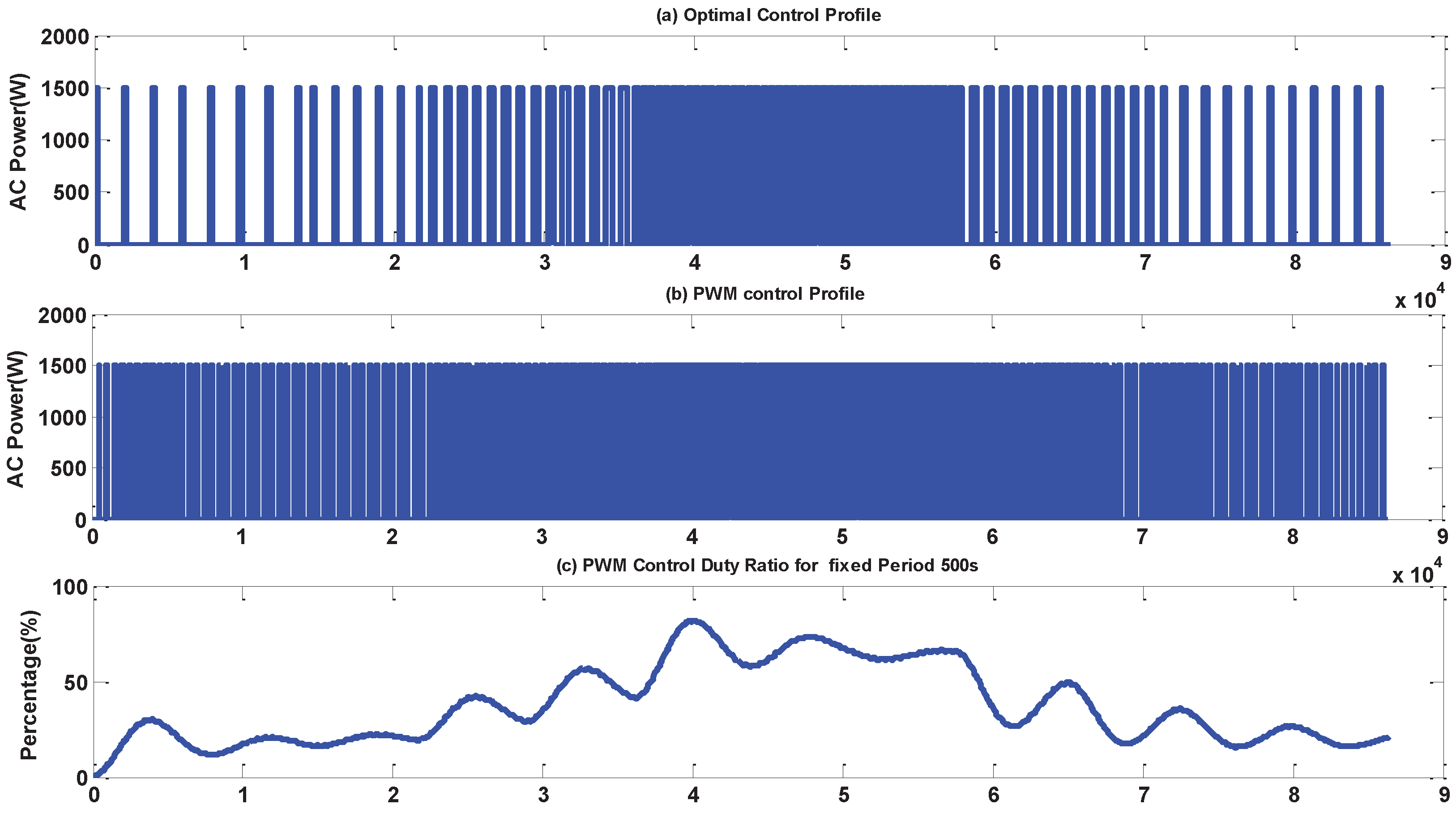
By investigating more details about the control variables of the control approaches, the power profile for the optimal control and the PWM control is shown in Figure 17a,b, respectively. The duty ratio profile of the PWM control is shown in Figure 17c. By comparing Figure 17a,b, it can be concluded that the optimal control has less pulses than the PWM control, and the cost due to switch is obviously reduced. From Figure 17c, we can see that the duty ratio is a continuous variable which changes according to the outdoor temperature profile, which means that the PWM control can smooth the transition in a better way that the conventional On-Off control, although it is not the optimum comparing to the proposed optimum control.
Based on the fixed period value (500 s) and corresponding duty ratio sampling in each time duration, the cost in terms of COP in (10) is calculated, and the cost comparison in the corresponding time period is shown in Table 4. From the table, we can see the proposed optimal control has less cost than the PWM control in each time duration, which means the proposed optimal control has a better control performance for multiple objectives, which consider both Coefficient of Performance, and AC compressor weariness due to On-Off switching.
4.3.2. Case 2- Cases through Three Hot Seasons in Doha of Qatar
To demonstrate the validity of the proposed scheme under three hot seasons in Qatar, complete yearly outdoor temperature data taken from our measurements, from June of 2018 to June of 2019, were used. As can been from Figure 18, the outdoor temperature is fully or partially over 25 degrees except from December to March. In other words, spring, summer, and autumn are all hot seasons in Qatar. Thus, AC cooling is essential and the proposed optimization scheme can be applied. Considering this diversity of the Qatar desert climate, profiles of three typical days in each season, which include 2019/8/6, 2018/11/6, 2019/5/6, were selected to validate the proposed scheme for the three seasons of summer, autumn, and Spring, respectively.
As the hottest month of the year in Qatar, August is a typical for AC cooling scenarios due to its high outdoor temperature and resulting cooling load. The validation results for the selected summer day in August are presented in Figure 19. The outdoor temperature profile shows that it varies from 32 C to 46 C in one summer day, which means that the gap between peak point and valley point is large and the AC needs to adaptively accommodate the corresponding time-variant cooling load. From the optimum temperature control profile, we can see that the oscillation period time at the peak point of the outdoor temperature is the shortest because it needs to generate the highest cooling effort. With 2-h interval time zone moving, the duty ratio and period time are both set as the best optimized value by the offline optimizations. Although the profile is not always close to the central of the target temperature of 25 C, the temperature variation range is within 1 C. This result demonstrates that the proposed AC control scheme can achieve the optimal cooling effect within the comfort level need of AC cooling.
The validation result for a typical autumn day, in November of 2018, is presented in Figure 20. As shown in the outdoor temperature profile, it changes from 27 C to 29 C in one autumn season day. This means that the gap during the same day is very small, and also, the cooling load is lighter compared to summer days. From the optimum temperature control profile, we can see that the oscillation period time is longer than the summer case because of the lighter cooling load. The control profile is always kept to approach the target 25 C with 1 C variation range. These results demonstrate the effectiveness of the proposed scheme during autumn days in Qatar.
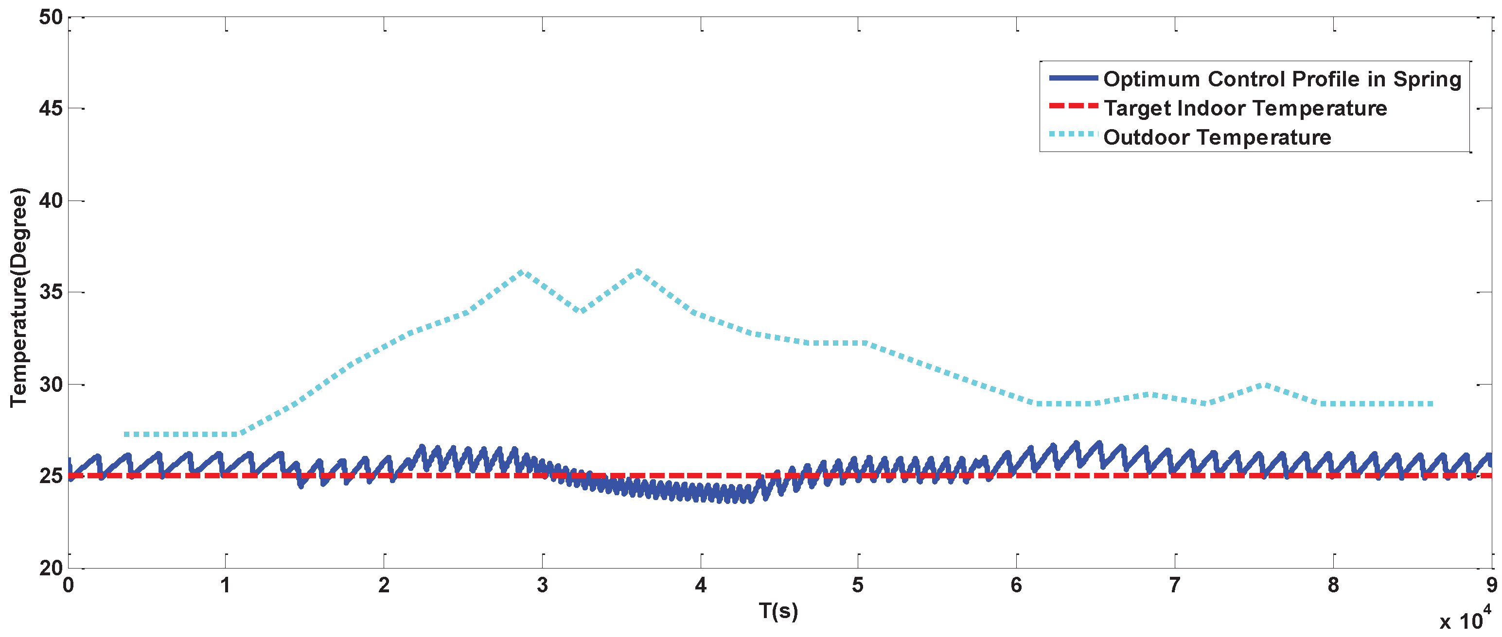
The validation result for a typical spring day, in May of 2019, is shown in Figure 21. The outdoor temperature changes from 27 C to 37 C in one spring season day. This means the gap during the same day is smaller compared to summer days, and also the cooling load is changing quickly within same day. From the optimum temperature control profile, we can see that the oscillation period time is set with a very different value range because the cooling load is changing with large value range. The control profile is a little off the target 25 C due to the large variations of AC control parameter tuning, but it still satisfy the comfort level by approaching the target 25 C within 2 C variation range. These results demonstrate the effectiveness of the proposed scheme under spring season days in Qatar.
Remark 3.
Because of the significance of Qatar’s extremely hot weather conditions, AC Optimization and control in this region is very different from other regions. Particular challenges such as large daily temperature peaks, heavy cooling load through the year, AC Group Consumption peaks, and local resident electricity consumption behaviours, also need to be considered. To address these challenges, effective optimization solutions are supposed to be applied for multiple objectives but not only COP and switching cost. Therefore, the needed optimization process will be more complicated, and accordingly, more advanced optimization theories such as optimization feasible zone, and tools including cloud-computing and super-computing are needed for future studies.
5. Conclusions
This paper presents a new optimal control strategy that improves existing conventional On-Off control for air conditioning under the harsh desert climate of Qatar. The optimum AC control is achieved based on an integration between off-line optimization and online adaptive control. The optimization process involves the use of a multiple objectives methodology driven by a cost function for maximum energy efficiency (COP) and minimized compressor weariness. This control scheme offers a practical trade-off between online and off-line optimization methods where the multiple objective optimization is achieved without excessive computational needs. By simulating several AC cooling scenarios, based on our experimental weather data from the outdoor test facility at Qatar Environment and Energy Research Institute, the resulting performance is very promising. More optimization objectives and factors such as sizing AC unit numbers, AC power fluctuations and impact to grid will be considered for future work.
Author Contributions
Conceptualization: M.A.-A., Z.C., S.A., Y.R.; Methodology, Validation, Data Curation: M.A.-A., Z.C.; Writing-Original Draft Preparation: M.A.-A., Z.C.; Writing-Review and Editing: M.A.-A., Z.C., S.A., Y.R. All authors have read and agreed to the published version of the manuscript.
Funding
This research received no external funding.
Acknowledgments
The authors thank the QEERI Outdoor Facility Team (Energy Center), particularly Dr. Benjamin Figgis, for the local weather data and technical support.
Conflicts of Interest
The authors declare no conflict of interest.
References
- Shaaban, K.; Muley, D. Investigation of weather impacts on pedestrian volumes. Transp. Res. Procedia 2016, 14, 115–122. [Google Scholar] [CrossRef] [Green Version]
- Guo, B.; Javed, W.; Figgis, B.; Mirza, T. Effect of dust and weather conditions on photovoltaic performance in Doha, Qatar. In Proceedings of the IEEE 2015 First Workshop on Smart Grid and Renewable Energy (SGRE), Doha, Qatar, 22–23 March 2015; pp. 1–6. [Google Scholar]
- Perez-Astudillo, D.; Bachour, D. Variability of measured global horizontal irradiation throughout Qatar. Solar Energy 2015, 119, 169–178. [Google Scholar] [CrossRef]
- Touati, A.; Hussain, S.J.; Touati, F.; Bouallegue, A. Effect of atmospheric turbulence on hybrid FSO/RF link availability under Qatar harsh climate. Int. J. Electron. Commun. Eng. 2015, 9, 902–908. [Google Scholar]
- Sim, L.F. Numerical modelling of a solar thermal cooling system under arid weather conditions. Renew. Energy 2014, 67, 186–191. [Google Scholar] [CrossRef]
- Ayoub, N.; Musharavati, F.; Pokharel, S.; Gabbar, H.A. Energy consumption and conservation practices in Qatar-A case study of a hotel building. Energy Build. 2014, 84, 55–69. [Google Scholar] [CrossRef]
- Touati, F.; Al-Hitmi, M.; Chowdhury, N.A.; Hamad, J.A.; Gonzales, A.J.S.P. Investigation of solar PV performance under Doha weather using a customized measurement and monitoring system. Renew. Energy 2016, 89, 564–577. [Google Scholar] [CrossRef]
- Sofotasiou, P.; Hughes, B.R.; Calautit, J.K. Qatar 2022: Facing the FIFA World Cup climatic and legacy challenges. Sustain. Cities Soc. 2015, 14, 16–30. [Google Scholar] [CrossRef]
- Shaaban, K.; Muley, D.; Elnashar, D. Evaluating the effect of seasonal variations on walking behaviour in a hot weather country using logistic regression. Int. J. Urban Sci. 2018, 22, 382–391. [Google Scholar] [CrossRef]
- Saffouri, F.; Bayram, I.S.; Koç, M. Quantifying the cost of cooling in qatar. In Proceedings of the 2017 9th IEEE-GCC Conference and Exhibition (GCCCE), Manama, Bahrain, 8–11 May 2017; pp. 1–9. [Google Scholar]
- Teather, K.; Hogan, N.; Critchley, K.; Gibson, M.; Craig, S.; Hill, J. Examining the links between air quality, climate change and respiratory health in Qatar. Avicenna 2013, 2013, 9. [Google Scholar] [CrossRef] [Green Version]
- Kassas, M. Modeling and simulation of residential HVAC systems energy consumption. Procedia Comput. Sci. 2015, 52, 754–763. [Google Scholar] [CrossRef] [Green Version]
- Deng, H.; Larsen, L.; Stoustrup, J.; Rasmussen, H. A novel method for control of systems with costs related to switching: Applications to air-condition systems. In Proceedings of the IEEE 2009 European Control Conference (ECC), Budapest, Hungary, 23–26 August 2009; pp. 1148–1154. [Google Scholar]
- Godina, R.; Rodrigues, E.M.; Pouresmaeil, E.; Catalão, J.P. Home HVAC energy management and optimization with model predictive control. In Proceedings of the 2017 IEEE International Conference on Environment and Electrical Engineering and 2017 IEEE Industrial and Commercial Power Systems Europe (EEEIC/I&CPS Europe), Milan, Italy, 6–9 June 2017; pp. 1–5. [Google Scholar]
- Di Felice, M.; Piroddi, L.; Leva, A.; Boer, A. Adaptive temperature control of a household refrigerator. In Proceedings of the IEEE 2009 American Control Conference, St. Louis, MO, USA, 10–12 June 2009; pp. 889–894. [Google Scholar]
- Martínez-Rosas, E.; Vasquez-Medrano, R.; Flores-Tlacuahuac, A. Modeling and simulation of lithium-ion batteries. Comput. Chem. Eng. 2011, 35, 1937–1948. [Google Scholar] [CrossRef]
- Dong, J.; Olama, M.; Kuruganti, T.; Nutaro, J.; Winstead, C.; Xue, Y.; Melin, A. Model predictive control of building on/off HVAC systems to compensate fluctuations in solar power generation. In Proceedings of the 2018 9th IEEE International Symposium on Power Electronics for Distributed Generation Systems (PEDG), Charlotte, NC, USA, 25–28 June 2018; pp. 1–5. [Google Scholar]
- Rehrl, J.; Horn, M. Temperature control for HVAC systems based on exact linearization and model predictive control. In Proceedings of the 2011 IEEE International Conference on Control Applications (CCA), Denver, CO, USA, 28–30 September 2011; pp. 1119–1124. [Google Scholar]
- Huang, G. Model predictive control of VAV zone thermal systems concerning bi-linearity and gain nonlinearity. Control. Eng. Pract. 2011, 19, 700–710. [Google Scholar] [CrossRef]
- Elliott, M.S. Decentralized Model Predictive Control of a Multiple Evaporator HVAC System. Master’s Thesis, Texas A & M University, College Station, TX, USA, 2008. [Google Scholar]
- Chen, W.; Chan, M.Y.; Deng, S.; Yan, H.; Weng, W. A direct expansion based enhanced dehumidification air conditioning system for improved year-round indoor humidity control in hot and humid climates. Build. Environ. 2018, 139, 95–109. [Google Scholar] [CrossRef]
- Jabarullah, N.H.; Shabbir, M.S.; Abbas, M.; Siddiqi, A.F.; Berti, S. Using random inquiry optimization method for provision of heat and cooling demand in hub systems for smart buildings. Sustain. Cities Soc. 2019, 47, 101475. [Google Scholar] [CrossRef]
- Esmaeilzadeh, A.; Zakerzadeh, M.R.; Koma, A.Y. The comparison of some advanced control methods for energy optimization and comfort management in buildings. Sustain. Cities Soc. 2018, 43, 601–623. [Google Scholar] [CrossRef]
- Afram, A.; Janabi-Sharifi, F. Theory and applications of HVAC control systems—A review of model predictive control (MPC). Build. Environ. 2014, 72, 343–355. [Google Scholar] [CrossRef]
- Moroşan, P.D.; Bourdais, R.; Dumur, D.; Buisson, J. Building temperature regulation using a distributed model predictive control. Energy Build. 2010, 42, 1445–1452. [Google Scholar] [CrossRef]
- Ma, Y.; Borrelli, F.; Hencey, B.; Coffey, B.; Bengea, S.; Haves, P. Model predictive control for the operation of building cooling systems. IEEE Trans. Control. Syst. Technol. 2011, 20, 796–803. [Google Scholar]
- Martinčević, A.; Vašak, M.; Lešić, V. Model predictive control for energy-saving and comfortable temperature control in buildings. In Proceedings of the IEEE 2016 24th Mediterranean Conference on Control and Automation (MED), Athens, Greece, 21–24 June 2016; pp. 298–303. [Google Scholar]
- Xu, M.; Li, S. Practical generalized predictive control with decentralized identification approach to HVAC systems. Energy Convers. Manag. 2007, 48, 292–299. [Google Scholar] [CrossRef]
- Silva, J.M.; Godina, R.; Rodrigues, E.M.; Pouresmaeil, E.; Catalão, J.P. Residential MPC controller performance in a household with PV microgeneration. In Proceedings of the 2017 IEEE Manchester PowerTech, Manchester, UK, 18–22 June 2017; pp. 1–6. [Google Scholar]
- Ascione, F.; Bianco, N.; De Stasio, C.; Mauro, G.M.; Vanoli, G.P. A new comprehensive approach for cost-optimal building design integrated with the multi-objective model predictive control of HVAC systems. Sustain. Cities Soc. 2017, 31, 136–150. [Google Scholar] [CrossRef]
- Péan, T.; Costa-Castelló, R.; Salom, J. Price and carbon-based energy flexibility of residential heating and cooling loads using model predictive control. Sustain. Cities Soc. 2019, 50, 101579. [Google Scholar] [CrossRef]
- Al-Azb, M.; Cen, Z.; Ahzi, S. Air-Conditioner On-Off optimization Control under Variant Ambient Condition. In Proceedings of the IEEE 2018 6th International Renewable and Sustainable Energy Conference (IRSEC), Rabat, Morocco, 5–8 December 2018; pp. 1–5. [Google Scholar]
Figure 1.
Average Min and Max Temperatures in Doha, Qatar for 2018.

Figure 2.
QEERI Outdoor Test facilities.

Figure 3.
Three-day outdoor profile in October of 2017.

Figure 4.
Thermal model of a house.

Figure 5.
Block diagram representation of state space model.

Figure 6.
Diagram of oscillation period dynamics.

Figure 7.
Flowchart of offline optimizations.

Figure 8.
Temperature profile discretization.

Figure 9.
Online AC control flowchart.

Figure 10.
Proposed Elman Neural Network Model structure.

Figure 11.
Cooling control profile comparison for different controller parameter settings.

Figure 12.
Offline optimization results under different outdoor temperatures.

Figure 13.
Outdoor Temperature prediction results.

Figure 14.
PWM control diagram.

Figure 15.
Online optimal control variables and parameters.

Figure 16.
Temperature control profile in a typical day with large temperature variations.

Figure 17.
PWM control process variables.

Figure 18.
Yearly Outdoor Temperature Profile from June of 2018 to June of 2019.

Figure 19.
Optimal control for typical summer day in Aug of 2018.

Figure 20.
Optimal control for typical autumn day in November 2018.

Figure 21.
Optimal control for typical spring day in May of 2019.


Table 1.
Parameters values of the thermal model and optimization.
| Parameter | A | B | E | R (C/W) | Cp (J/KgC) | m(kg) | Q | |
|---|---|---|---|---|---|---|---|---|
| Value | −2.00123 × 10 | 4.4028 × 10 | 0.002 | 0.022 | 2 | 1005 | 222 | 300 |
Table 2.
Performance comparison by Cost-saving.
| AC Cooling Control Strategies | Initial House Temperature | Period | Cost Value | Cost Saving |
|---|---|---|---|---|
| Case1 | 38 | 1595 | 3.4606 | 55.45% |
| Case2 | 29 | 300 | 2.2074 | 30.16% |
| Optimum Case | 34 | 595 | 1.5416 | N/A |
Table 3.
Optimization control parameters.
| Outdoor Temperature | Minimum Cost J | Period (T) | Duty Ratio () |
|---|---|---|---|
| 28 | 0.8585 | 1585 | 0.1090 |
| 30 | 0.5927 | 2400 | 0.2780 |
| 32 | 2.1917 | 595 | 0.2575 |
| 34 | 1.5416 | 595 | 0.3070 |
| 36 | 1.4318 | 595 | 0.3565 |
| 38 | 1.9049 | 595 | 0.4060 |
| 40 | 3.0049 | 595 | 0.4555 |
| 42 | 3.8368 | 595 | 0.5545 |
| 44 | 3.0705 | 595 | 0.6040 |
Table 4.
Cost comparison between PWM control and the proposed optimal control.
| Time Duration | Duty Ratio (%) | Cost of PWM Control | Cost of Optimal Control |
|---|---|---|---|
| 0 AM–2 AM | 1 | 14.85 | 1.1420 |
| 2 AM–4 AM | 11.76 | 7.77 | 1.1420 |
| 4 AM–6 AM | 16.02 | 1.75 | 1.3436 |
| 6 AM–8 AM | 37.90 | 4.59 | 2.0533 |
| 8 AM–10 AM | 45.61 | 11.06 | 2.8456 |
| 10 AM–12 AM | 64.68 | 6.26 | 5.3890 |
| 12 AM–2 PM | 66.02 | 14.67 | 5.3890 |
| 2 PM–4 PM | 61.07 | 112.89 | 3.0836 |
| 4 PM–6 PM | 33.24 | 56.58 | 2.1577 |
| 6 PM–8 PM | 19.01 | 10.07 | 2.5015 |
| 8 PM–10 PM | 16.43 | 12.33 | 2.2423 |
| 10 PM–12 PM | 17.02 | 29.89 | 1.3436 |
© 2020 by the authors. Licensee MDPI, Basel, Switzerland. This article is an open access article distributed under the terms and conditions of the Creative Commons Attribution (CC BY) license (http://creativecommons.org/licenses/by/4.0/).
Share and Cite
MDPI and ACS Style
Al-Azba, M.; Cen, Z.; Remond, Y.; Ahzi, S. An Optimal Air-Conditioner On-Off Control Scheme under Extremely Hot Weather Conditions. Energies 2020, 13, 1021. https://doi.org/10.3390/en13051021
AMA Style
Al-Azba M, Cen Z, Remond Y, Ahzi S. An Optimal Air-Conditioner On-Off Control Scheme under Extremely Hot Weather Conditions. Energies. 2020; 13(5):1021. https://doi.org/10.3390/en13051021
Chicago/Turabian StyleAl-Azba, Mohammed, Zhaohui Cen, Yves Remond, and Said Ahzi. 2020. "An Optimal Air-Conditioner On-Off Control Scheme under Extremely Hot Weather Conditions" Energies 13, no. 5: 1021. https://doi.org/10.3390/en13051021
Note that from the first issue of 2016, this journal uses article numbers instead of page numbers. See further details here.