Development of a Bio-Solar House Model for Egyptian Conditions
by
 , ,
, ,
El-Sayed Khater
1 ,
,
Taha Ashour
1,
Samir Ali
1,
Manar Saad
1,
Jasna Todic
2,
Jutta Hollands
2 and
Azra Korjenic
2,* 1
Agriculture Engineering Department, Faculty of Agriculture, Benha University, Moshtohor, Toukh 13736, Kalubia, Egypt
2
Research Unit of Ecological Building Technologies, Institute of Material Technology, Building Physics and Building Ecology, Faculty of Civil Engineering, Vienna University of Technology Karlsplatz 13/207-3, A-1040 Vienna, Austria
*
Author to whom correspondence should be addressed.
Energies 2020, 13(4), 817; https://doi.org/10.3390/en13040817
Submission received: 13 January 2020
/
Revised: 7 February 2020
/
Accepted: 10 February 2020
/
Published: 13 February 2020
(This article belongs to the Special Issue Biomass Energy Systems)
Abstract
:The need for heating and cooling in traditional housing is becoming increasingly disadvantageous regarding high energy costs. But what is more concerning is the impact on our environment. The main goal of this paper is studying the prospects of using renewable energy for heating and cooling houses through an integrated bio-solar system in order to solve the energy scarcity problem. For this purpose, a simulation model for a bio-solar house made from different materials (walls made of bricks with straw bales and a roof made of concrete with straw bales) was developed successively in accordance with the energy balance and renewable energies such as biogas and solar energy were applied. This approach enabled an enhancement of the main factors affecting the performance of a building in terms of saving energy. The model was able to predict the energy requirements for heating and cooling of houses, the energy gained by a solar collector and by a biogas digester as well as the energy requirement for heating the biogas digester. Also, the purpose of this paper is to validate this developed simulation model by measuring energy requirements for heating of houses and solar radiation for solar collectors. The model is a simulation model for the bio-solar house with its three main parts—a straw house, a solar collector and a biogas digester. This paper demonstrates the values of the performed measurements and compares them to the theoretical, predicted values. The comparison indicates that the predicted energy requirements for the heating of buildings were a close approximation to the measured values. Another relevant deduction of the validation was the fact that the solar collector delivered the highest heat gain on 21st of June.
1. Introduction
Energy scarcity is becoming a problem that cannot be ignored. Egypt’s energy balance for 2007 indicates that the largest share of final energy consumption occurs in the industrial sector (34.2%), followed by transportation (24.2%), residential buildings (18.8%) and agriculture and mining (4.7%), which altogether makes 81.9% of the total consumption. According to the International Energy Agency [1], the energy consumption measured in the residential buildings of different countries in 2004 was divided into 4% for cooking, 5% for lighting, 17% for water heating, 20% for appliances and 54% for space heating. Energy Information Administration pointed out that the consumed amounts of petroleum started to exceed the produced amounts in Egypt from the last of 2011. This contrast became especially conspicuous in 2014 where on a daily basis only 710,000 barrels were produced while 770,000 barrels were consumed. These findings lead to the conclusion that studies on decreasing energy consumption in residential and agriculture sectors are essential steps towards finding solutions to the energy scarcity problem.
To improve the performance and welfare of the people living by regulating the environmental condition inside their buildings. The physical environment is affected by many factors such as temperature, relative humidity and air quality. The temperature is considered as the most important factors in environmental control in buildings [2]. There are some other factors the affecting the environment in buildings such as ventilation, illumination, photoperiod, humidity, noise levels and aerial pollutant levels. Maintaining the temperature inside the building within a desired range by adjusting ventilation, heating and cooling rates is the simplest way to manage the building’s environment [3]. Energetic analyses can enable a comparison of all processing units with modern production approach or even alter the production lines [4]. Insulation is one of the instruments for energy management and the reduction of energy losses in the form of heat especially in cold areas with long winters. Managing equipment and consumption patterns in order to reduce the utilized energy and results in cost reduction and is therefore an effective approach. All these aspects and the rapid increase in production costs encouraged producers to pay more attention to their energy consumption [5].
The main aim of models is to assess the developers and customers communicate and to test case generation or automatic of the developed system. [6]. A modeling language consists of the description of its syntax, including well-formedness rules and its semantics [7]. Using formal semantics of a language is commonly agreed about it because it avoids problems like misunderstandings between people and lack of interoperability between tools. Also, semantics can be used for verification purposes. However, many languages are often specified through their syntax only and lack a precise semantics beyond informal explanations. Unified model language (UML) is a prominent example which has been standardized without a formal semantics [8,9].
One of the main problems of traditional housing are the rising costs for heating and cooling. Considering the ongoing rise of temperatures due to global warming, it is more and more difficult for people to abstain from consumption of energy for these purposes, especially in areas of the world where these global warming related fluctuations are beyond unbearable. According to Korjenic [10], the majority of building owners, custodians and engineers, as well as building users, tend to react to increasing outdoor temperatures by increasing energy consumption for cooling in order to safeguard thermal comfort under all conditions. In order to break this vicious circle, we need to explore environment-friendly alternatives and ensure that these methods find their way to the public and into practical application.
Assessing the environmental and energy related impacts of buildings is completed by using a building energy performances simulation (BEPS) [11]. These tools deal with all the most important phenomena occurring in the building [12,13] and around it and the used energy efficiency techniques or renewable energy sources [14]. The utilization of BEPS tools is highly recommended for the design of the next generation of buildings (Nearly Zero Energy Buildings—NZEBs), for the promotion of renewable energy technologies integration and for the building energy diagnosis [15]. BEPS tools enable the designers to optimize the thermal performance, thermal comfort and energy performance of the building. Computer simulation is commonly used in predicting the thermal comfort and indoor air quality as affected by outdoor temperature and air distribution patterns inside the buildings [16]. This is particularly significant when developing innovative strategies such as incorporating natural ventilation.
This study focuses on a special model of a bio-solar house set in Egypt under hot climate conditions. The motivation behind the development of the mentioned model was a detailed study on necessary heating and cooling energy values applied on an ecologically friendly system that could lead to a reduction of energy consumption especially in hot areas such as Egypt. Therefore, the main aim of this paper is therefore to study the possibility of using renewable energy for heating and cooling houses through an integrated bio-solar system in order to reduce the costs and solve the energy scarcity problem. To achieve that, a bio-solar system model of a building which can predict the energy gains and losses from buildings under Egyptian climate conditions was developed and alternative energy types of the bio-solar system were studied.
2. Model Development
Heat balance was performed on bio-solar houses to determine system energy gains, losses and the demand for air conditioning of the system. To maintain the required conditions inside of the building space, the conditioning system must overcome the energy loads which are imposed by the climatic conditions outside of the building and also the factors inside of the building itself.
2.1. System Description
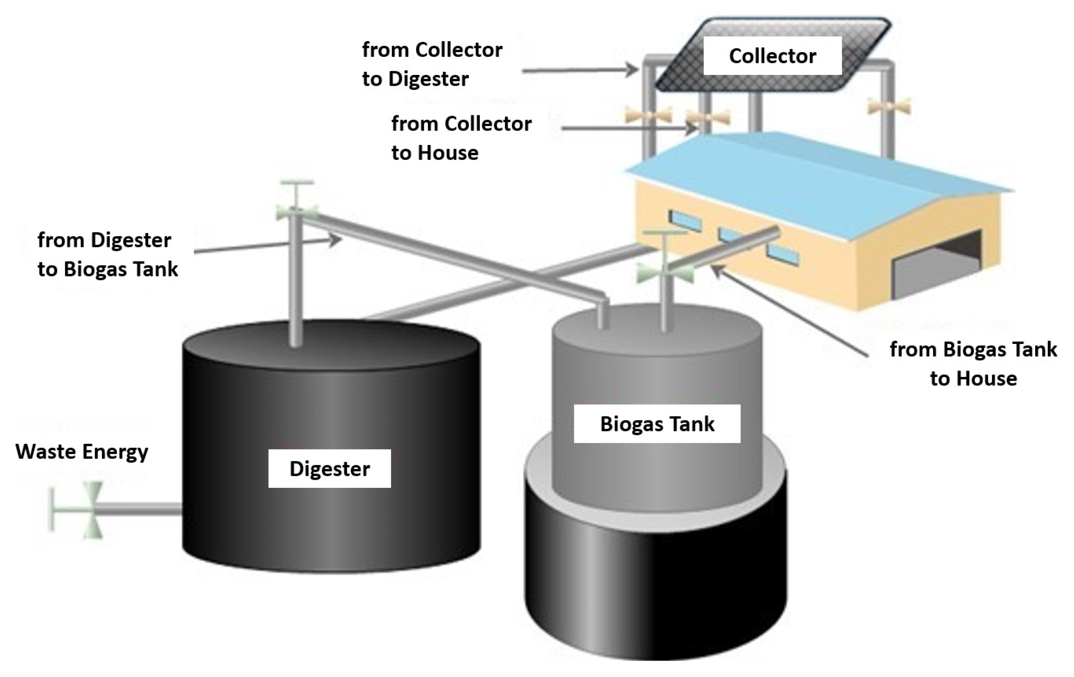
The bio-solar house system consists of three main parts—the straw house, a solar collector and a biogas digester as shown in Figure 1. Straw bales are used as a building material or as insulation material for the original construction material. Using biogas and solar energy permits three possible air conditioning systems of the building:
- Buildings heated by solar energy.
- Buildings heated by both solar and biogas energy (biogas digester heated by solar energy).
- Buildings heated by biogas energy that is heated by solar energy.
2.2. Mathematical Model
The following assumptions for the development of the present model are made:
- The model is based on steady-state conditions.
- The temperature of air is uniform across the whole building.
- The density and heat capacity of the air are constant.
- The temperature gradients within the constructions are negligible.
- The building walls have negligible heat capacity.
- The Egyptian time zone is GMT/UTC±2, so LSM for Egypt is 30° according to Reference [17].
- The distance between absorbent plate and glass cover is assumed to be 3 mm.
- Clearness number is assumed to be 0.7 along the lines of [18].
- The absorber plate temperature is assumed to be 90 °C or 363.15 °K and the glass cover temperature is assumed to be equal to the ambient temperature.
- The internal gains in the digester are to be neglected.
- The collector tilt angle is 45°.
2.2.1. Houses Energy Requirements
Energy balance was performed on the house. The energy exchange due to both external and internal energy loads is shown in Figure 2. The external energy loads are transmission, fenestration, perimeter, ventilation and infiltration. The internal loads are occupants, lighting and appliances. The internal energy loads and the fenestration always count as sources of heat gain. Ventilation, infiltration, perimeter and heat transmission loads cause heat loss in winter months and heat gain in summer months. Equation (1) presents the energy balance components of the house.
with
Q—total energy at any time in the house in J
Qs—heat gains by people in W
Qfens.—heat gains by fenestration in W
Qlight—heat gain by light in W
Qappliances—heat gain by appliances in W
Qconv.—heat exchange with the air by convection in W
Qcond.—heat exchange with the wall by conduction in W
Qp—heat exchange by perimeter of floor in W
Total fenestration heat gain by the sun radiation splitting into three parts can be calculated as followed Equations (2)–(5) [17]:
with
Qb—direct solar beam heat gain in W
Qd—diffuse solar heat gain in W
Qc—conductive heat gain in W
Awindows – windows area in m2
ED—direct irradiance
Ed—diffuse irradiance
Er—ground-reflected irradiance
SHGC—solar heat gain coefficient
IAC—inside shading attenuation coefficient (= 1.0 without an inside shading device)
U—overall U-factor in w m−2 k−1
Tout—temperature of the outer surface in K
Tin—temperature of the inner surface in K
The radiation emitted by the sun travels through the vacuum of space unaltered. For the determination of the surface direct irradiance (ED) the following Equation (6) is needed [17]:
where
EDN—direct normal irradiance in W
θ—solar incident angle in degrees
The direct normal irradiance can be determined with Equation (7) [13]:
where
β—solar altitude angle, degrees
Cn—clearness number
A—apparent solar constant in W m−2
B—atmospheric extinction coefficient (dimensionless)
The angle that a ray of light falling on the irradiated surface creates with the line normal to the irradiated surface is called the angle of incidence θ. Its value is determined by [17] demonstrated in Equation (8):
with
γ—surface-solar azimuth angle in degrees
∑—surface tilt angle from the horizontal plane (also called slope) in degrees
L—local latitude angle (negative in the southern hemisphere) in degrees
δ—solar declination angle in degrees
H—hour angle in degrees
ASHRAE [19] mentioned that the earth’s equatorial plane is tilted at an angle of 23.45° to the orbital plane, so the solar declination δ is determined according to the following Equation (10) provides sufficient accuracy [19]:
with
n—day of the year
The hour angle (H) is determined according to Equation (11) as follows:
where
AST—apparent solar time in hours
The apparent solar time (AST), as determined by a solar time sundial, varies somewhat from the mean time of a clock kept running at a uniform rate. This variation is called the equation of time (ET) and is approximated by the following Equations (12) and (13) [19]:
With ET expressed in minutes and
The apparent solar time (AST) is calculated as follows (Equation (14)) [17]:
where
LST—local standard time in hours
LON—longitude of site in degrees of Greenwich
LSM—longitude of local standard time meridian in degrees of Greenwich (negative in the western hemisphere)
The standard meridian longitude is related to the time zone as follows in Equation (15) [17]:
TZ—time zone, expressed in hours ahead or behind coordinated universal time UTC.
The surface-solar azimuth angle (γ) is defined as the angular difference between the solar azimuth ϕ and the surface azimuth ψ as shown in Equation (16) [17]:
The solar azimuth () is calculated as follows:
The apparent solar radiation (A) and the atmospheric extinction coefficient (B) are calculated by the following equations Equations (18) and (19):
For vertical surfaces the diffuse irradiance Ed coming from the sky is calculated following Equation (20) [18]:
However, for surfaces other than vertical the calculation is carried out as shown in Equation (21):
with
C—sky diffuse factor (dimensionless)
Y—ratio of sky diffuse on a vertical surface to the sky diffuse on a horizontal surface (dimensionless)
The ratio of the sky diffuse irradiation on vertical surfaces to the sky diffuse irradiation on horizontal surfaces can be calculated with the following Equation (23) [20]:
—ground reflectivity
The conduction of heat between the inner surface and the outer surface of the building was calculated by Equation (25):
with
k—thermal conductivity coefficient in W m−1 K−1
A—the surface area in m2
z—thickness of wall surface in m
The heat transferred through convection can be calculated using Newton’s Law of cooling, which is shown in Equation (26).
with
h—heat transfer coefficient in W m−2 K−1
Nusselt number (Nu) correlations are traditionally used to predict a heat transfer coefficient within the Equation (27):
with
Lc—characteristic length of the surface in m
The characteristic length for a rectangular block is given as follows in Equation (28) [21]:
When it comes to free convective surfaces, the Nusselt number is related to another dimensionless number, the Rayleigh number (Ra), through empirical correlations. The Rayleigh number is:
with
g—gravitational acceleration, 9.81 m s−2
β—coefficient of thermal expansion in K−1
v—kinematic viscosity of the fluid in m2 s−1
μ—dynamitic viscosity of the air in m−1 s−1
Cp—specific heat of air in J kg−1K−1
The extinction coefficient is given by Equations (30) and (31):
For free convection, the Nusselt number is given for horizontal or vertical planes, pipes, rectangular blocks and spheres as follows in Equations (32) and (33) [21]:
If Ra between 104 and 108
If Ra between 108 and 1012
In cases where wind is present (i.e., forced convection), different flat plate correlations could be used but they run the risk of being unsuitable. The following Nusselt number correlation for mixed laminar and turbulent flow regions (for 5 × 10⁵ < Re < 108) can be used [22].
with
Re—Reynold’s number
The previous equation is valid for Prandtl numbers between 0.6 to 60. The Reynold’s number, Re, is a dimensionless number representing the ratio of inertial to viscous forces in the boundary layer of the fluid. It can be calculated according to Equation (35):
with
V—velocity of the air, m s−1
The occupants heat gains are distinguished in sensible heat gains. They are calculated according to Equation (36) [18].
with
qs, per—sensible heat gain per person in W kg−1
N—Number of occupants
Even though occupant density is low, occupancy loads should be estimated nevertheless. Sensible heat gain per sedentary occupant is assumed to be 67 W. To prevent gross oversizing, the number of occupants should not be overestimated. Recent census studies recommend that the total number of occupants should be based on two persons for the first bedroom, plus one person for each additional bedroom. The occupancy load should then be distributed equally among the living areas because the maximum load occurs when most of the residents occupy these areas [17].
The heat transfer according to perimeter can be estimated by Equation (37) for both unheated and heated slab floors [17]:
with
F—heat loss coefficient per foot of perimeter in W m−1 K−1
P—perimeter of floor in m
The heat gain from electric lighting may be calculated by Equation (38) [20]:
with
W—total light wattage in W
Ful—lighting use factor
Fsa—lighting special allowance factor
The lighting use factor is the ratio of the wattage in use, for the conditions under which the load estimate is being made, to the total installed wattage.
Heat gain by equipment is calculated with Equation (39) [22]:
2.2.2. Digester Energy Analysis
The digester has a cylinder shape. According to Fourier’s law and Newton’s law of cooling for convection, the thermal resistances are calculated as mentioned in Equation (26). Furthermore, according to Newton’s law of cooling, the convection heat coefficient is given by Equation (27). From the air out of the digester the heat transfer is from free convection so, the Nusselt number is given by Equations (32) and (33). But, from the digestate inside the building the heat transfer is from forced convection. The Nusselt number is given in Equations (40) and (41) according to [15]:
- Laminar flow:
- Turbulent flow:
The energy required of the digester depends on energy needed for the conditioning system and the bio-solar houses system used as shown below:
- If the used system includes a building heated with solar energy and unheated biogas energy or a building heated with solar energy and biogas energy which is heated with solar energy, then the total energy needed from the digester on daily basis should be:= (Avg. yearly rate required for conditioning) × (24- Avg. yearly sunshine hours)/1000.
- If the used system involves a building heated with biogas energy which is heated with solar energy, then the total energy needed from the digester on a daily basis should be:= (Avg. yearly rate required for conditioning) (24)/1000.
The volume of the biogas digester depends on this needed energy. The heating value of non-purified biogas is 6.5 kWh m−3 [23]. Necessary biogas quantity will be:
- Biogas quantity needed (m3 day−1) = Energy needed from digester/6.5.
- Required feedstock rate (kg day−1) = Biogas daily quantity/Biogas yield.
Therefore:
added water rate = required feedstock rate × (total solids − 8)/8
Whereas 8 is the optimum total solids ratio for the AD process. By considering the density of digesting mix equal to water density (1000 kg m−3), the volume of digester will be:
digester volume = (water + feedstock rate daily) * retention time/1000
2.2.3. Solar Collector Performance Analysis
The basic equation for calculating the performance of collectors is given in Equation (42) [24]:
with
Qu—useful heat gained by collector per unit of aperture area in W m−2
It—total irradiation of collector in W m−2
τ—transmittance of cover times
α—absorptance of plate
UL—upward heat loss coefficient in W m−2 K−1
tp—Temperature of the absorber plate in K
tout—temperature of the atmosphere in K
ASHRAE [25] suggested that an additional term, the collector heat removal factor FR, should be introduced in order to permit the use of the fluid inlet temperature. This additional term is added as shown in Equation (43).
with
FR—ratio of the heat delivered by the collector to the heat that would be delivered if the absorber were at tfi.
Assuming that the collector efficiency is (qu/Itθ) = 80%, the FR ratio can be calculated in the following manner [18]:
The total solar irradiation Et Equation (45) is the sum of the direct component from Equation (6) and the diffuse component in Equation (20) and Equation (21) coming from the sky plus whatever amount of reflected shortwave radiation Er may reach the surface from the earth or from adjacent surfaces [24]:
The overall heat loss coefficient is given by the following expression [24]:
with
Ut—top heat loss coefficient in W m−2 K−1
Ub—bottom heat loss coefficient in W m−2 K−1
Ue—edges heat loss coefficient in W m−2 K−1
The coefficient of heat loss from the upper surface of the solar collector with a single cover (Ut) can be determined with Equation (47).
with
hpc—heat transfer coefficient of natural convection
hrpc—radiation heat transfer coefficient from the absorber to the glass cover
hcw—convective heat transfer coefficient between the glass and the environment
hrcw—radiation heat transfer coefficient between glass cover and sky
For the heat transfer coefficient of natural convection (hpc) the following Equation (48) applies:
with
L—distance between the absorber plate and glass cover
The convective heat transfer coefficient between the absorber plate and the glass is calculated from the Nusselt number according to the following Equation (49) [26]:
The radiation heat transfer coefficient from the absorber to the glass cover (hrpc) can be stated as in Equation (50) [27]:
The convective heat transfer coefficient between the glass and the environment (hcw) is calculated according to Equation (51) [28]:
Radiation heat transfer coefficient between glass cover and sky (hrcw) is determined by Equation (52):
A simple relationship, which ignores vapor pressure of the atmosphere, may be used to estimate the apparent sky temperature demonstrated in Equation (53) [29]:
The empirical relations for Ub and Ue coefficients are mentioned by [29] as follows in Equations (54) and (55):
3. Model Approach
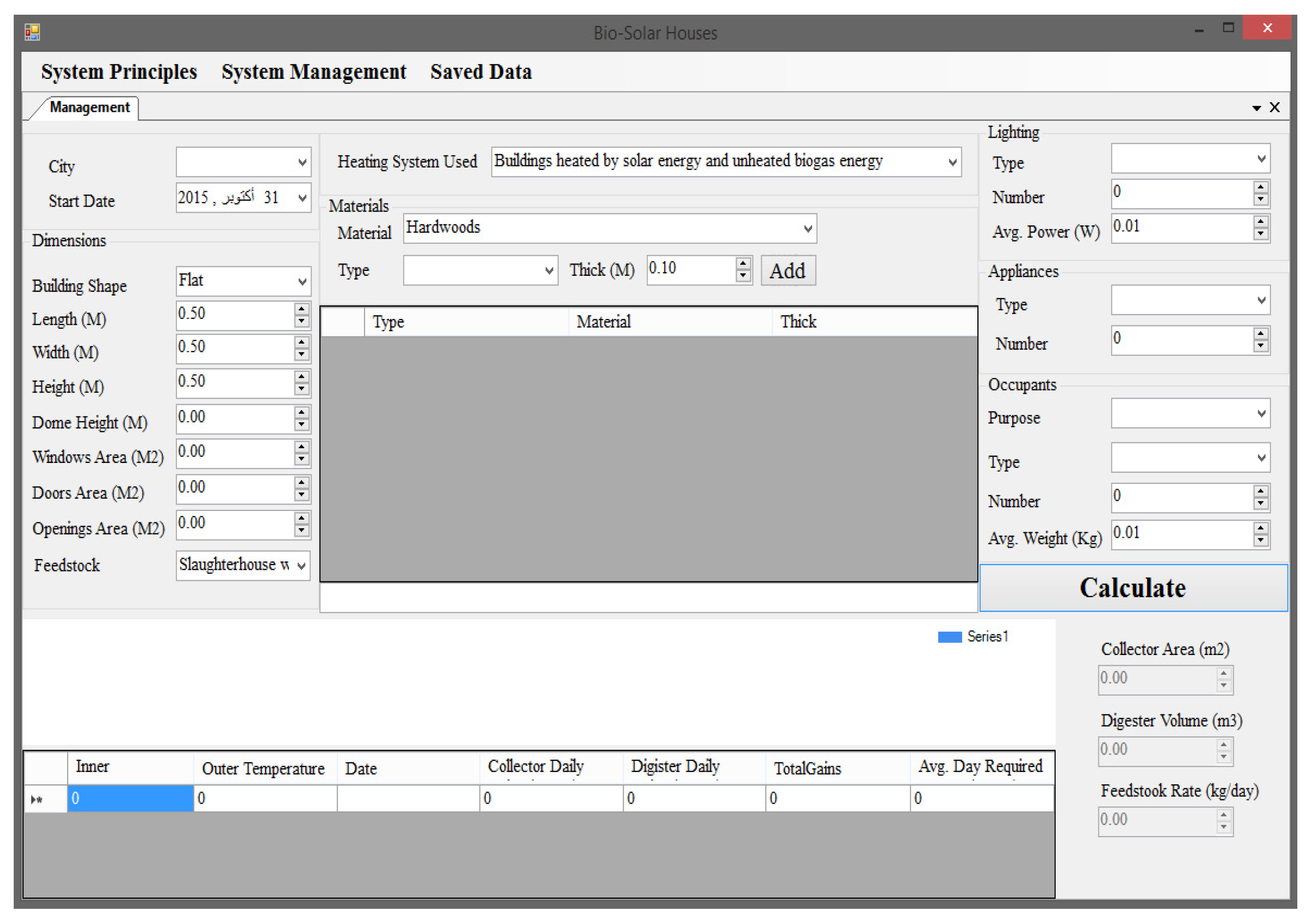
All computational procedures of the model were carried out using Microsoft Visual Basic 2013. The program’s graphical user interface with the data input window below can be seen in Figure 3. The computer program focused on heat balance for predicting the temperature and energy gain or loss of the house. Figure 4 shows the user approach in the model. The parameters used in the model which were obtained from literature are listed in Table 1.
The model is designed to consist of three parts:
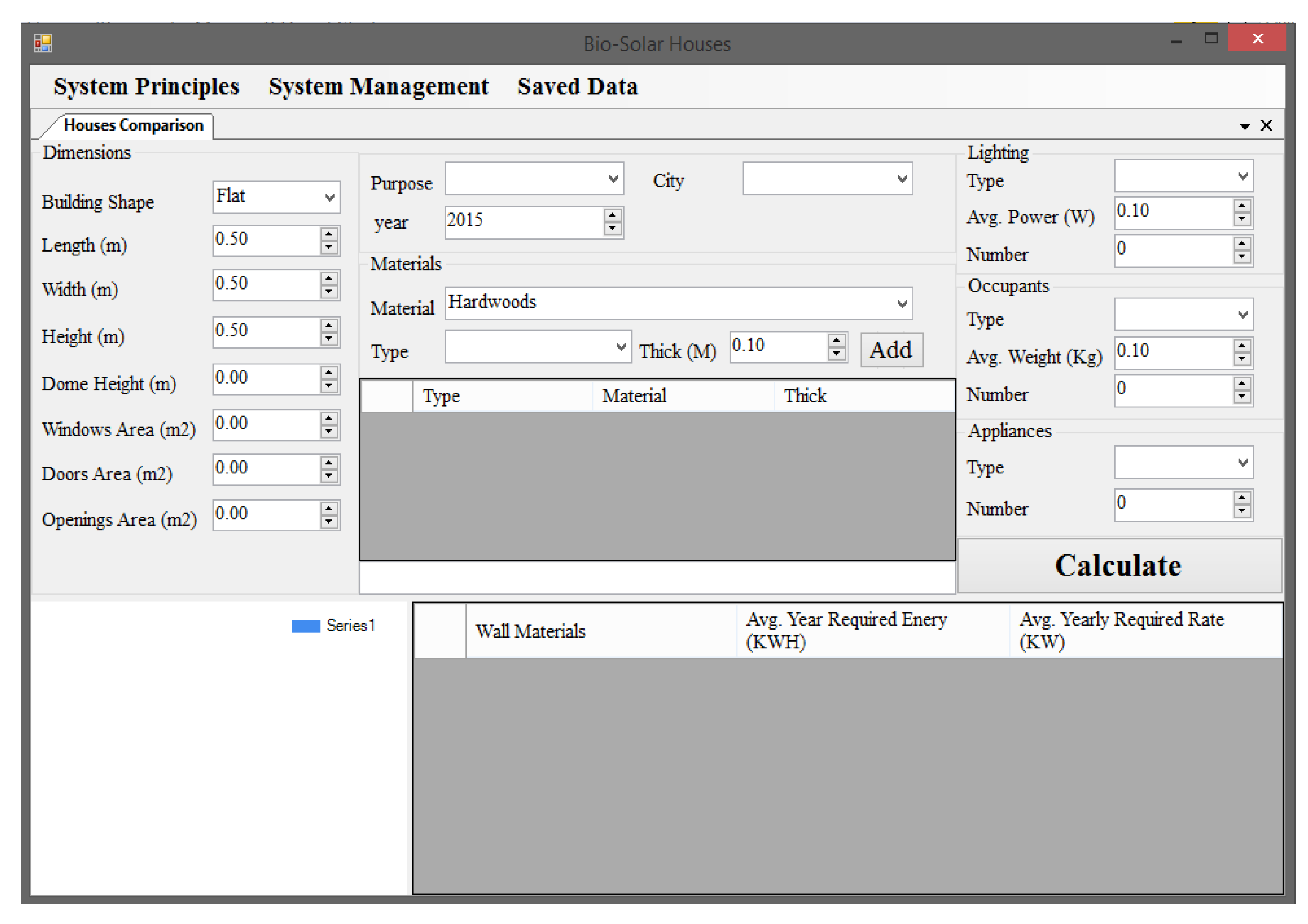
The first part was devoted to houses’ performance form as shown in Figure 5. This form was used to determine the difference between building with straw and other materials by calculating the energy quantity needed in a specific building (specific area) for conditioning.
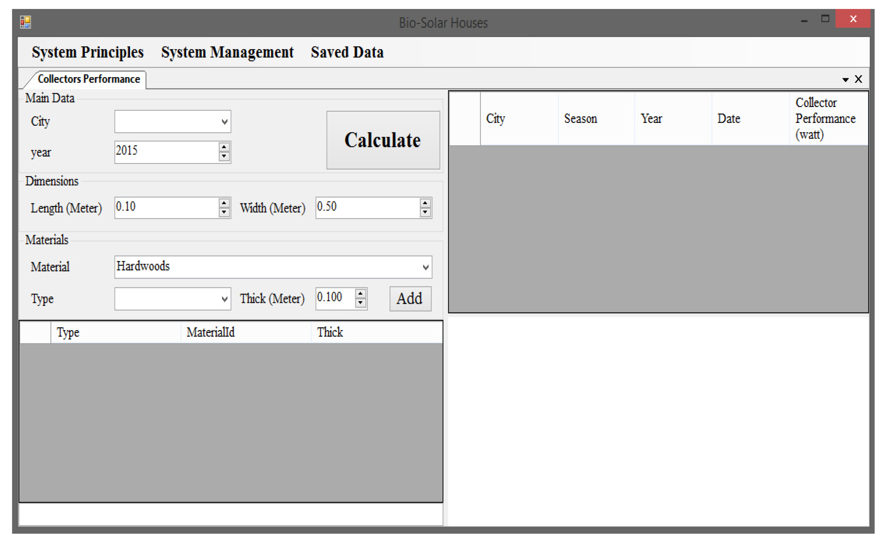
The second part was devoted to solar collectors’ form as shown in Figure 6. This form calculates the thermal energy rate that can be gained and stored when using solar collectors in specific areas.
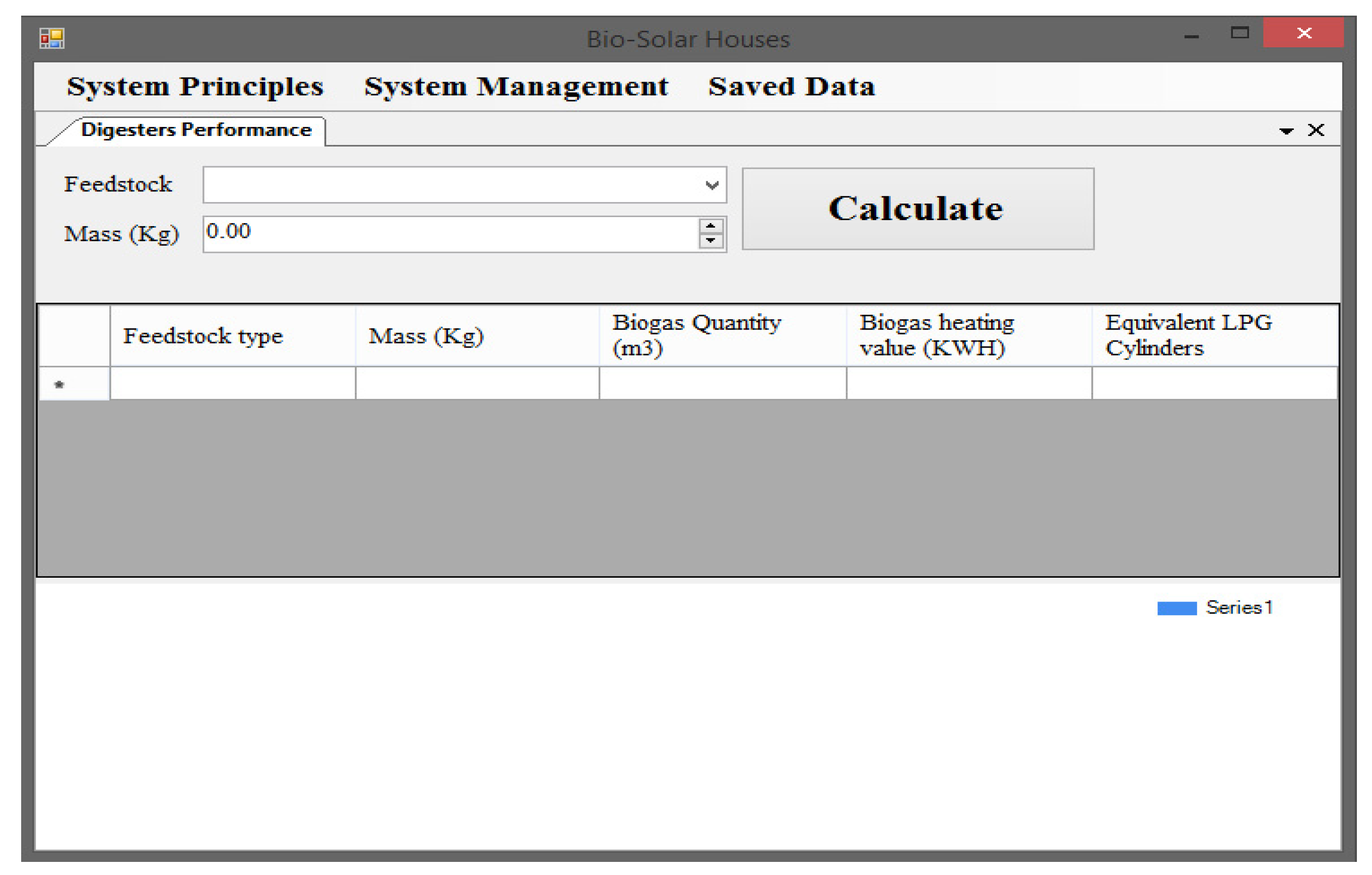
The third part was devoted to the biogas digester form as shown in Figure 7. This form calculates the thermal energy that can be gained from the biogas digester by calculating the amount of biogas produced from a certain type of feedstock and its heating value (kWh) and then equivalent LPG (liquefied petroleum gas) cylinders.
Figure 8 shows the result of using the bio-solar houses system by calculating the heat requirements and gains of the system throughout its working season. The form also calculates the digester’s volume and collector area needed for conditioning buildings.
4. Procedures
The objective of this study is the requirement for the surface of the collector and the volume of the digester in order to provide the bio-solar house with the energy required for heating.
4.1. Description of the Experimental Bio-Solar House
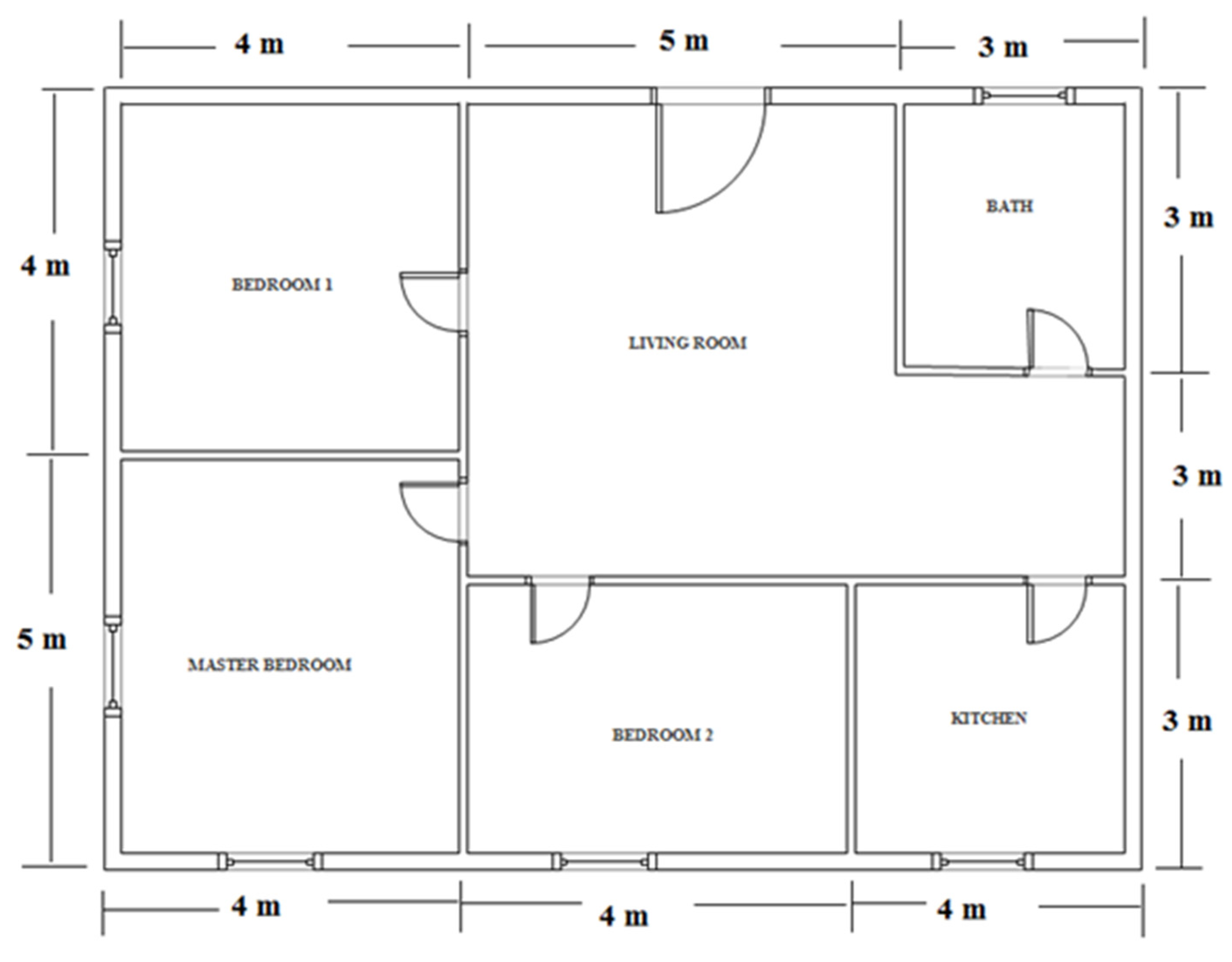
The experiment was carried out on a single-family detached house (Figure 9) at Toukh city, El-Qalubia Governorate, Egypt. It consists of walls made of bricks and straw bales and a concrete roof with straw bales. The bio-solar house is 12.0 m long, 9.0 m wide and 3.0 m high. It has glass windows and wooden doors. The surfaces of windows and doors are 6.0 and 12.0 m2, respectively. The thickness of the brick walls, the concrete roof, the glass windows and wood doors are 0.20, 0.1, 0.006 and 0.05 m, respectively. The surface of windows and doors is 6.0 and 12.0 m2, respectively. The bio-solar house is provided with 8 LED lamps (12 Watt each) for lighting. The number of persons for each house is four.
The energy used for heating the house was recorded daily in order to calculate the energy requirement for heating. The recorded energy consumption was used to validate the predicted energy from the energy balance model.
This system provides a solar collector and a biogas digester. Table 2 shows the specifications of the bio-solar house.
This study was done using collector performance formed in the model. Table 3 shows the data of the used collector. The solar radiation was recorded from the weather station in Moshtohor. The recorded solar radiation was used to validate the predicted solar radiation from the model.
4.2. Case Studies on the Bio-Solar House
The cases, which have been studied on the bio-solar house are the following:
- Heating the house with solar energy.
- Heating the house and the biogas digester with solar energy during daylight and with biogas at night (temperature of the biogas digester is 309.15 K and retention time is 35 days).
- Heating the house and biogas digester with solar energy during daylight and with biogas at night (temperature of biogas digester is 322.15 K and retention time is 17.5 days).
- Heating the house with biogas while the biogas digester is heated by solar energy (temperature of biogas digester is 309.15 K and retention time is 35 days).
- Heating the house with biogas while the biogas digester is heated by solar energy (temperature of biogas digester is 322.15 K and retention time is 17.5 days).
5. Results and Discussion
5.1. Model Experimentation
5.1.1. Solar Collector Area and Biogas Digester Volume Requirements
Table 4 shows the required area of solar collectors and the necessary volume of the biogas digester to provide the required energy for different case studies for the bio-solar house. It could be seen that the solar collector areas required for the first, second, third, fourth and fifth case study were 177.17, 179.06, 180.31, 4.25 and 8.50 m2. The volume of the biogas digester in order to provide the required energy for the bio-solar house were 9.76, 4.56, 2.28, 9.15 and 4.56 m3, respectively.
The results indicate that only the fourth and the fifth case can be applied. In the first, second and third case the collector area is larger than the roof area of the bio-solar house.
5.1.2. Results of Case Studies during Winter Season
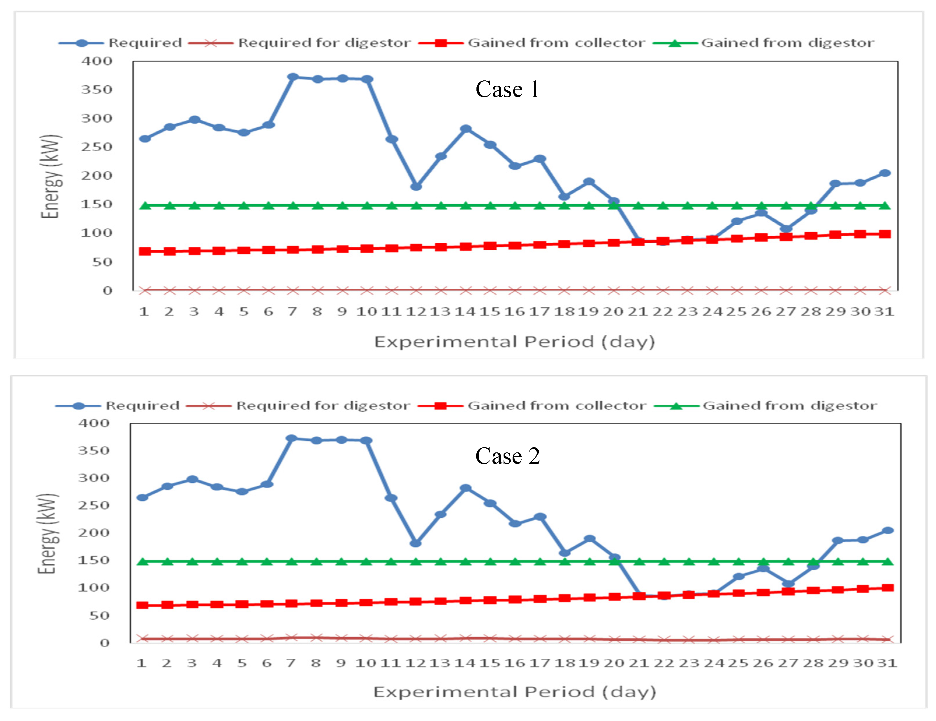
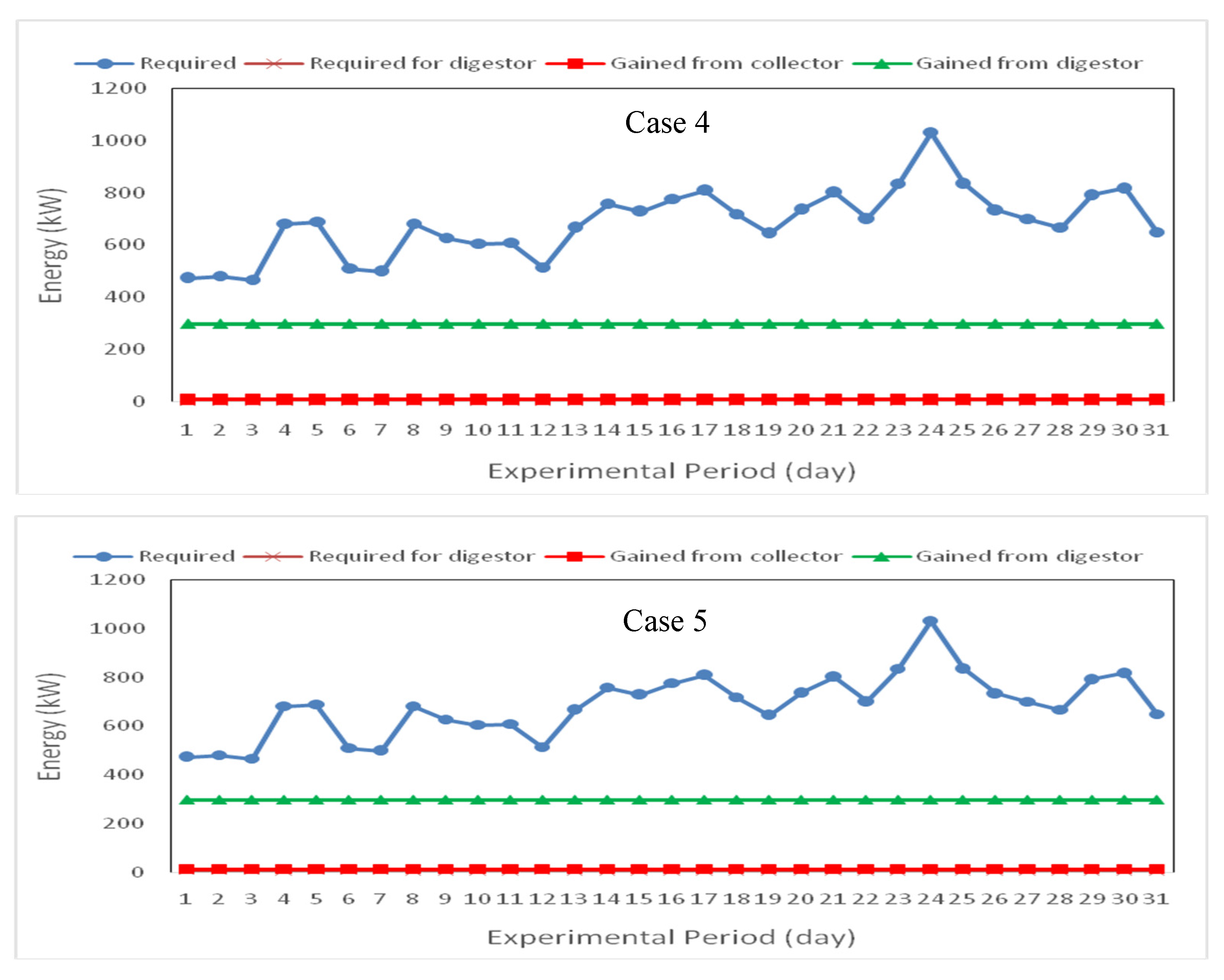
Figure 10 shows the energy requirement for heating and energy gained by solar collector and biogas digester for different bio-solar housing during the winter season (January) in Toukh city. The results indicate that the energy requirements for heating the house ranged from 85.07 to 373.63 kW for all studied cases. The results show that the energy gained by the solar collector ranged from 68.10 to 98.43, 68.62 to 99.72, 69.22 to 100.58, 1.21 to 1.76 and 2.01 to 2.93 kW for first, second, third, fourth and fifth case of heating the bio-solar house, respectively. The average energy gained by the biogas digester was 148.87, 148.87, 148.87, 297.75 and 297.75 kW for first, second, third, fourth and fifth case, respectively.
The results also show that the energy requirements for heating the biogas digester ranged from 5.37 to 9.66, 8.02 to 11.56, 7.58 to 13.11 and 11.01 to 15.69 kW for second, third, fourth and fifth case of heating, respectively, during the winter season (January) in Toukh city.
5.1.3. Results of Case Studies during Summer Season
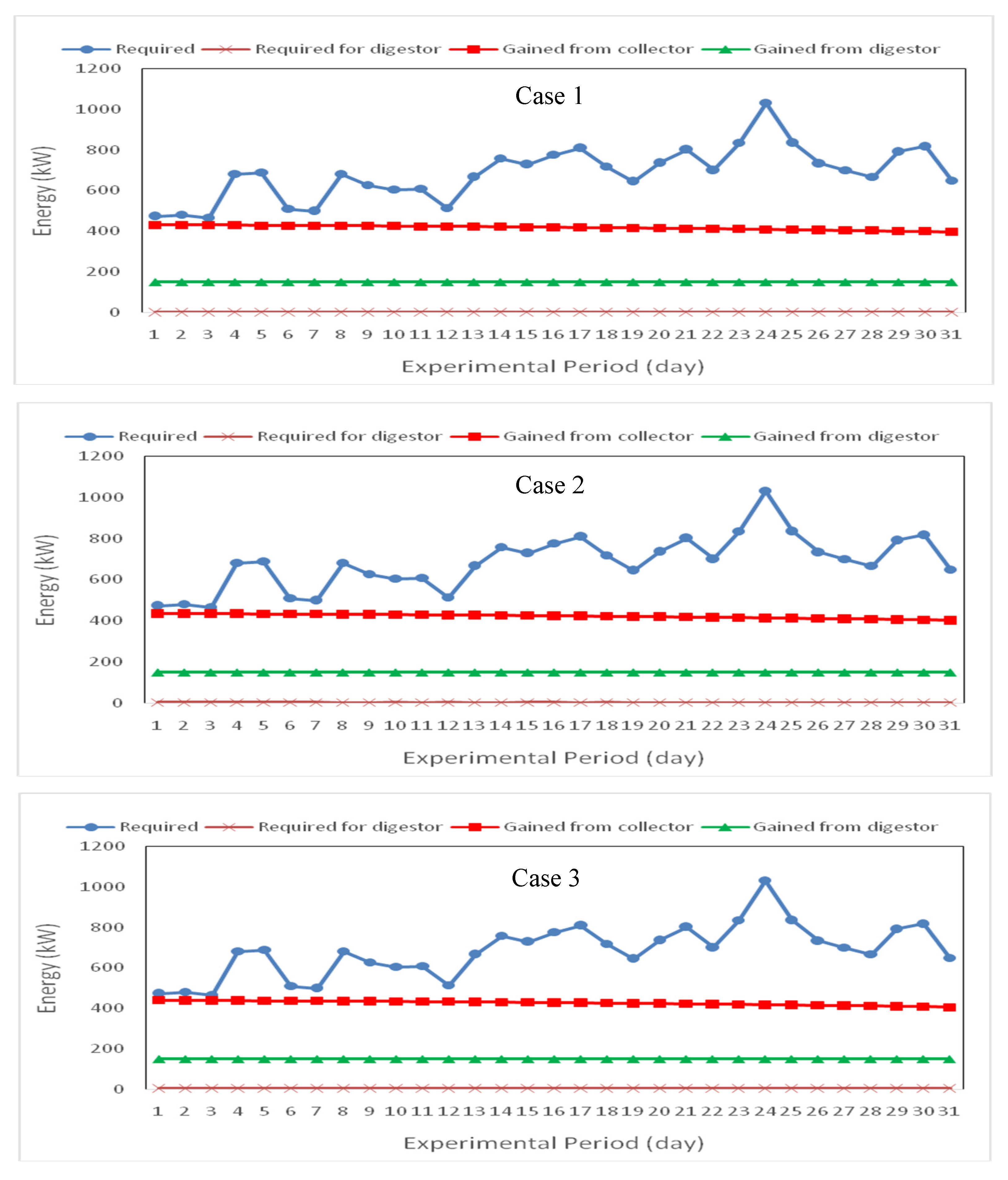
Figure 11 shows the energy requirement for cooling and the energy gained by the solar collector and biogas digester for a different bio-solar house during the summer season (July) in Toukh city. The results demonstrate that the energy requirements for cooling the house ranged from 466.08 to 1031.76 kW for all case studies of the bio-solar house. The energy gained by the solar collector ranged from 396.61 to 430.52, 401.84 to 436.19, 405.30 to 439.95, 7.09 to 7.70 and 11.79 to 12.80 kW for first, second, third, fourth and fifth bio-solar house, respectively. The average energy gained by the biogas digester was 148.87, 148.87, 148.87, 297.75 and 297.75 kW for first, second, third, fourth and fifth case, respectively.
The results also show that the energy requirement for heating the biogas digester ranged from 1.14 to 2.27, 3.52 to 5.18, 1.54 to 3.06 and 4.75 to 7.00 kW for second, third, fourth and fifth bio-solar house, respectively.
5.1.4. Digester Performance
Figure 12 shows the amount of biogas production from different types of waste. It can be seen that the biogas production was 12.0, 210.0, 560.0, 180.0, 72.8, 70.0, 20.0, 65.0, 185.0, 610.0, 110.0, 47.0, 432.3, 126.0, 126.0, 56.0, 686.0, 267.8 and 72.0 m3 per 1000 kg for pig slurry, maize silage, maize grain, grass silage, fresh grass, cattle-dung, cattle-slurry, poultry, whole wheat crop, wheat grain, food waste, sewage sludge, old bread, chicken litter/dung, horse manure, clover, chaff and residuals from vegetables, respectively. The highest value of biogas production (686.0 m3 per 1000 kg) was found by the use of clover waste, while the lowest value of biogas production (12 m3 per 1000 kg) was found for pig slurry.
5.1.5. Solar Collector Performance
Figure 13 shows the heat gain by the solar collector during different days of the year in Toukh city. The results show that the heat gained by the solar collector ranged from 66.015 to 305.735 W m2. The highest value of heat gained by solar collector (305.735 W m2) was reached on 21 June 2017 whereas the lowest value of heat gained by the solar collector (66.015 W m−2) was reached on 21 December 2017.
5.2. Model Validation
5.2.1. Energy Requirement for Heating the House
Figure 14 shows the predicted and the measured energy requirement for heating the house during the winter season (January). It can be seen that the predicted energy requirements were in a reasonable agreement with those measured, seeing as they ranged from 89.65 to 390.12 kW experimentally, while ranging 85.07 to 373.63 kW theoretically.
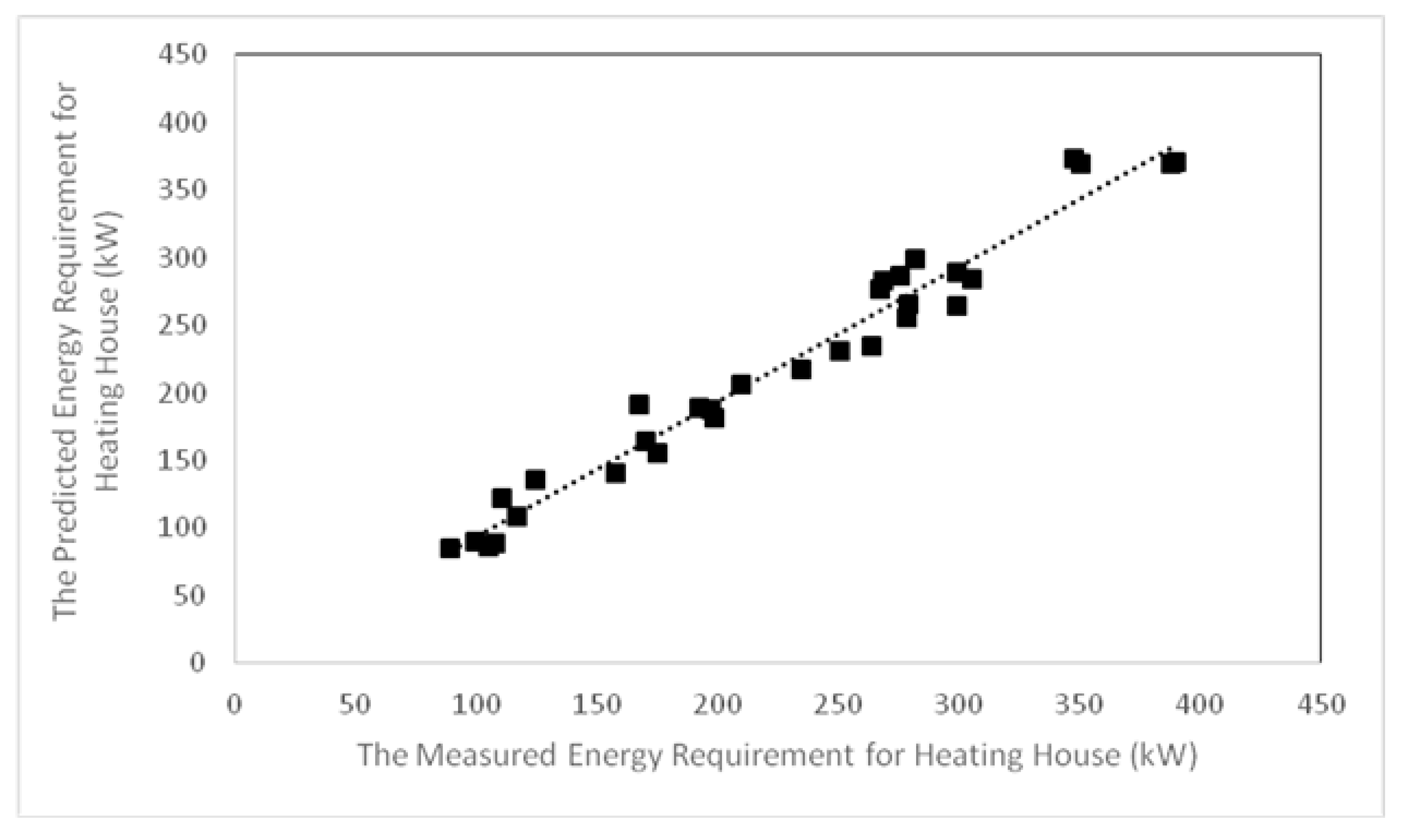
The variations between the predicted and measured energy requirement for heating the house during the winter season (January) are shown in Figure 15. The best fit for the relationship between the predicted and the measured value could be described as follows in Equation (56):
where
Ep is the predicted energy requirement for heating the house in KW
EM is the measured energy requirement for heating the house in KW
5.2.2. Solar Radiation
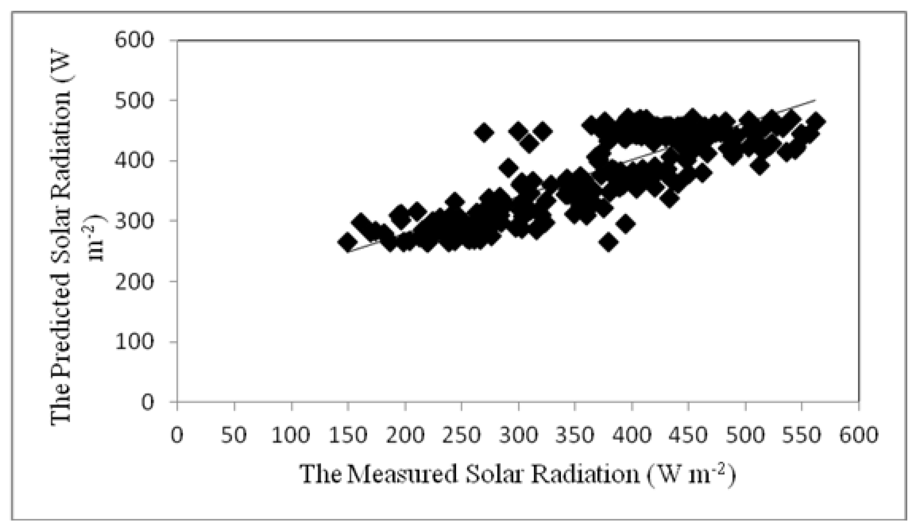
Figure 16 shows the predicted and the measured solar radiation from solar collector. It can be noticed that the average solar radiation predicted by the model was in good agreement with the radiation measured by the system, seeing as it ranged from 161.00 to 561.85 W m−2 experimentally while ranging from 264.88 to 470.68 W m−2 theoretically. The stratification of solar radiation has been predicted well for the system.
The variations between the predicted and measured solar radiation from the solar collector are shown in Figure 17. The best fit for the relationship between the predicted and the measured value can be determined with the following equation:
where
Ip - predicted solar radiation in W m−2
IM -measured solar radiation in W m−2
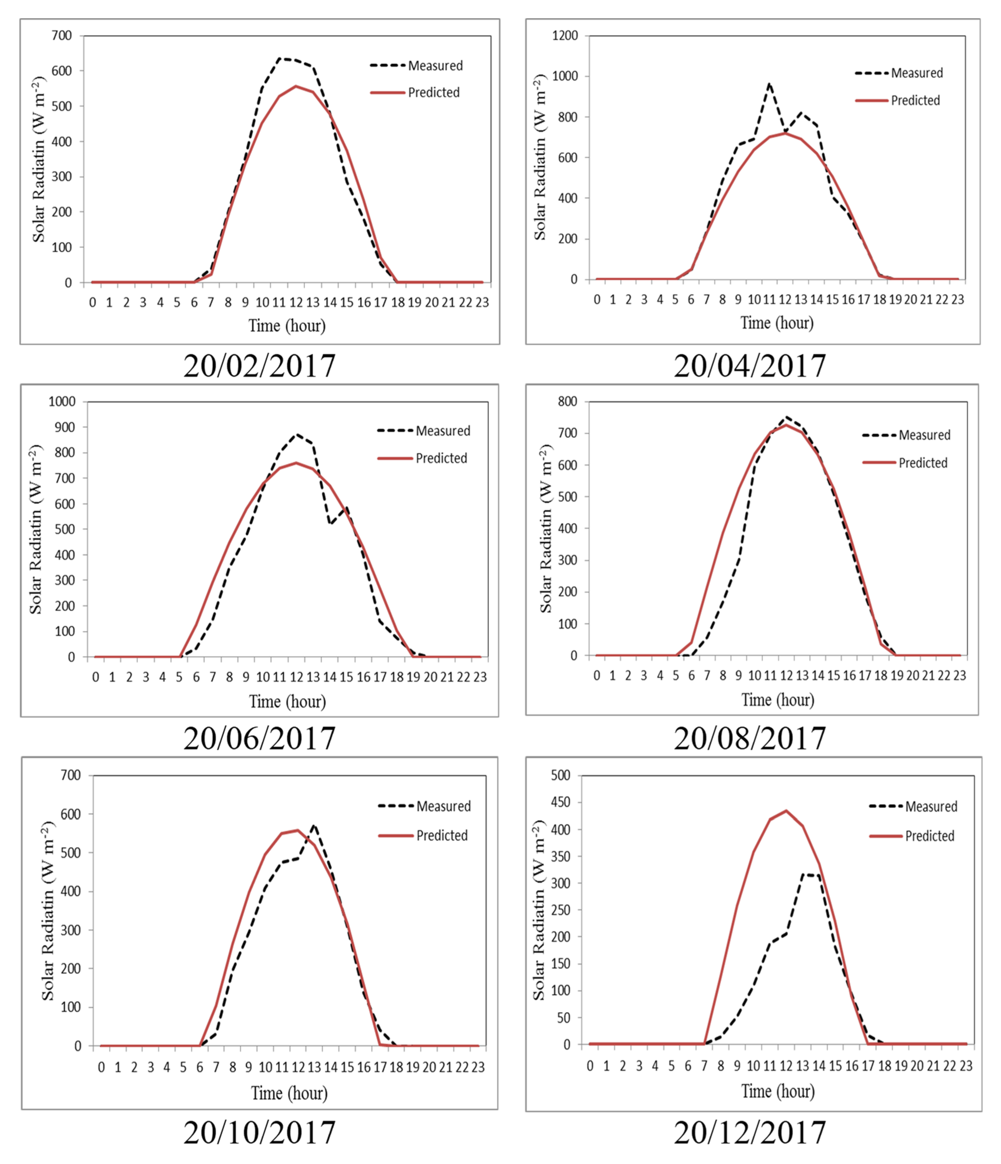
Figure 18 shows the predicted and the measured hourly average solar radiation from the solar collector. The average hourly solar radiation predicted by the model was in good agreement with the radiation measured by the system. It ranged from 39 to 634, 22 to 970, 16 to 872, 58 to 752, 32 to 575 and 14 to 315 W m−2 experimentally on 20/2, 20/4, 20/6, 20/8, 20/10 and 20/12/2017, respectively, whereas the theoretical values ranged from 24.1 to 452.08, 17.45 to 720.80, 102.45 to 760.38, 36.07 to 726.10, 4.03 to 558.37 and 0.33 to 434.11 W m−2 on 20/2, 20/4, 20/6, 20/8, 20/10 and 20/12/2017, respectively.
6. Conclusions
A simulation model for the bio-solar house was developed successively according to energy balance to optimize the main factors affecting the performance of buildings built with different materials (the walls are made of bricks with straw bales and the roof is made of concrete with straw bales). Applying renewable energies such as biogas and solar energy to this system results in energy savings and the reduction of energy related costs. The model was able to predict the energy requirements for heating and cooling of the houses, the energy gained by the solar collector, the energy gained by the biogas digester and the energy requirements for heating the biogas digester. Also, carrying out an experiment to validate the model results through measuring energy requirement for heating house and the solar radiation for the solar collectors. The most important results obtained within the frames of validation can be summarized as follows:
- The required solar collector area and the biogas digester volume for providing the bio-solar house with the required energy were 177.17, 179.06, 180.31, 4.25 and 8.50 m2 and 9.76, 4.56, 2.28, 9.15 and 4.56 m3 for first, second, third, fourth and fifth case study, respectively.
- The highest values of energy gained by the solar collector during winter and summer seasons were 100.58 and 439.95 kW were found for third case study, respectively, while the lowest values of energy gained were 2.01 and 11.79 kW was found for fifth case study, respectively.
- The average energy gained by the biogas digester was 148.87, 148.87, 148.87, 297.75 and 297.75 kW for first, second, third, fourth and fifth bio-solar house, respectively, during winter and summer season.
- The energy requirement for heating the biogas digester during winter season ranged from 5.37 to 9.66, 8.02 to 11.56, 7.58 to 13.11 and 11.01 to 15.69 kW for second, third, fourth and fifth study case, respectively, while ranging from 1.14 to 2.27, 3.52 to 5.18, 1.54 to 3.06 and 4.75 to 7.00 kW for first, second, third, fourth and fifth bio-solar house, respectively, during summer season.
- The highest value of biogas production (686.0 m3 per 1000 kg) was reached using the clover waste, whereas the lowest value of biogas production (12 m3 per 1000 kg) was reached using pig slurry.
- The heat gained from the solar collector ranged from 66.015 to 305.735 W m2 during different days of the year in Toukh city.
- The predicted energy requirements and solar radiation were in a reasonable agreement with the measured ones. The energy requirements ranged from 89.65 to 390.12 kW experimentally, whereas theoretically the values ranged from 85.07 to 373.63 kW. The solar radiation ranged from 161.00 to 561.85 W m2 experimentally, while the theoretical values ranged from 264.88 to 470.68 W m2.
- Further studies on renewable energies utilization in heating and cooling buildings and recommend. Economical evaluation is recommended in further studies.
Author Contributions
T.A.: conceptualization, methodology, validation, formal analysis, investigation, writing original draft preparation; E.-S.K.: conceptualization, methodology, validation, formal analysis, investigation, writing original draft preparation; S.A.: Software, validation, methodology, supervision; M.S.: conceptualization, methodology, validation, formal analysis, investigation, writing original draft preparation; J.T.: Formal analysis, Writing reviewed and editing; J.H.: Formal analysis, Writing reviewed and editing; A.K.: Formal analysis, Writing reviewed and editing, supervision, project administration. All authors have read and agreed to the published version of the manuscript.
Funding
Open Access Funding by TU Wien.
Acknowledgments
The authors acknowledge TU Wien Library for financial support through its Open Access Funding Program and the Support and Development of Scientific Research Center, Benha University.
Conflicts of Interest
The authors declare no conflict of interest.
References
- International Energy Agency. Energy Efficiency Requirements in Building Codes, Energy Efficiency Policies for New Buildings; IEA Information Paper; International Energy Agency: Paris, France, 2008; pp. 1–85. [Google Scholar]
- Tungarayasub, I. A Bio-Solar House for Northern Thailand. Master’s Thesis, University of Massachusetts Lowell, Lowell, MA, USA, 2004. [Google Scholar]
- McMullan, R. Environmental Science in Buildings; Palgrave Macmillan: London, UK, 2002. [Google Scholar]
- Jekayinfa, S.O. Energetic Analysis of Poultry Processing Operations. Leonardo J. Sci. 2007, 10, 77–92. [Google Scholar]
- Alam, M.S.; Alam, M.R.; Islam, K.K. Energy Flow in Agriculture: Bangladesh. Am. J. Environ. Sci. 2005, 1, 213–220. [Google Scholar] [CrossRef]
- Grönniger, H.; Ringert, J.; Rumpe, B. System model-based definition of modeling language semantics. In Proceedings of the FMOODS/FORTE 2009, LNCS 5522, Lisbon, Portugal, 9–12 June 2009; pp. 152–166. Available online: www.se-rwth.de/publications (accessed on 9 December 2019).
- Harel, D.; Rumpe, B. Meaningful Modeling: What’s the Semantics of “Semantics”? Computer 2004, 37, 64–72. [Google Scholar] [CrossRef]
- France, R.; Evans, A.; Lano, K.; Rumpe, B. The UML as a formal modeling notation. Comput. Stand. Interfaces 1998, 19, 325–334. [Google Scholar] [CrossRef] [Green Version]
- Breu, R.; Grosu, R.; Huber, F.; Rumpe, B.; Schwerin, W. Towards a Precise Semantics for Object-Oriented Modeling Techniques. In Proceedings of the ECOOP 1997 Workshop on Precise Semantics for Object-Oriented Modeling Techniques, Jyväskylä, Finland, 9–13 June 1997; Kilov, H., Rumpe, B., Eds.; TUM-I9725. Technische Universitat Munchen: München, Germany, 1997; pp. 53–59. [Google Scholar]
- Berger, T.; Amann, C.; Formayer, H.; Korjenic, A.; Pospischal, B.; Neururer, C.; Smutny, R. Impacts of climate change upon cooling and heating energy demand of office buildings in Vienna, Austria. Energy Build. 2014, 80, 517–530. [Google Scholar] [CrossRef]
- Negendahl, K. Building performance simulation in the early design stage: An introduction to integrated dynamic models. Autom. Constr. 2015, 54, 39–53. [Google Scholar] [CrossRef]
- Szalay, Z.; Zöld, A. Definition of nearly zero-energy building requirements based on a large building sample. Energy Policy 2014, 74, 510–521. [Google Scholar] [CrossRef]
- Nembrini, J.; Samberger, S.; Labelle, G. Parametric scripting for early design performance simulation. Energy Build. 2014, 68, 786–798. [Google Scholar] [CrossRef]
- Todorović, M.S. BPS, energy efficiency and renewable energy sources for buildings greening and zero energy cities planning: Harmony and ethics of sustainability. Energy Build. 2012, 48, 180–189. [Google Scholar] [CrossRef]
- Diakaki, C.; Grigoroudis, E.; Kolokotsa, D. Towards a multi-objective optimization approach for improving energy efficiency in buildings. Energy Build. 2008, 40, 1747–1754. [Google Scholar] [CrossRef]
- Cook, M.; Yang, T.; Cropper, P. Thermal Comfort in Naturally Ventilated Classrooms: Application of Coupled Simulation Models Building Energy Research Group; Loughborough University: Loughborough, UK; Institute of Energy and Sustainable Development, De Montfort University: Leicester, UK, 2011; pp. 14–16. [Google Scholar]
- ASHRAE. Handbook Heating, Ventilating, and Air-Conditioning Application; ASHRAE (American Society of Heating, Refrigerating and Air-Conditioning Engineers): Atlanta, GA, USA, 2009. [Google Scholar]
- Ibrahim, A.; El-Sebaii, A.A.; Ramadan, M.R.I.; El-Broullesy, S.M. Estimation of Solar Irradiance on Inclined Surfaces Facing South in Tanta, Egypt. Int. J. Renew. Energy Res. 2011, 1, 18–25. [Google Scholar]
- Crawley, D.B.; Hand, J.W.; Kummert, M.; Griffith, B.T. Contrasting the capabilities of building energy performance simulation programs. Build. Environ. 2008, 43, 661–673. [Google Scholar] [CrossRef] [Green Version]
- ASHRAE. Handbook Heating, Ventilating, and Air-Conditioning Application; ASHRAE (American Society of Heating, Refrigerating and Air-Conditioning Engineers): Atlanta, GA, USA, 2001. [Google Scholar]
- Holman, J.P. Heat Transfer; McGraw-Hill: New York, NY, USA, 1997; p. 696. [Google Scholar]
- Arora, C.P. Refrigeration and Air Conditioning, 2nd ed.; McGraw-Hill: New Dehli, India, 2006. [Google Scholar]
- Petersson, A.; Wellinger, A. Biogas Upgrading Technologies—Developements and Innovations; IEA Bioenergy: Paris, France, 2014. [Google Scholar]
- ASHRAE. Handbook Heating, Ventilating, and Air-Conditioning System and Equipement; ASHRAE (American Society of Heating, Refrigerating and Air-Conditioning Engineers): Atlanta, GA, USA, 2003. [Google Scholar]
- ASHRAE. Applications of Solar Energy for Heating and Cooling of Buildings; ASHRAE (American Society of Heating, Refrigerating and Air-Conditioning Engineers): Atlanta, GA, USA, 1997. [Google Scholar]
- Hollands, K.G.T.; Unny, T.E.; Raithby, G.D.; Konicek, L. Free Convective Heat Transfer across Inclined Air Layers. J. Heat Transf. 1976, 98, 189–193. [Google Scholar] [CrossRef]
- Duffie, J.A.; Beckman, W.A. Solar Engineering of Thermal Processes, 4th ed.; WILEY: New York, NY, USA, 2013. [Google Scholar]
- Ali, I.; Senthilkumar, R.; Mahendren, R. Modelling of Solar Still Using Granular Activated Carbon in Matlab. Bonfring Int. J. Power Syst. Integr. Circuits 2011, 1, 5–10. [Google Scholar]
- ASHRAE. Thermal Environmental Conditions for Human Occupancy; ASHRAE (American Society of Heating, Refrigerating and Air-Conditioning Engineers): Atlanta, GA, USA, 2010. [Google Scholar]
Figure 1.
Bio-solar house system.

Figure 2.
Energy balance of house.
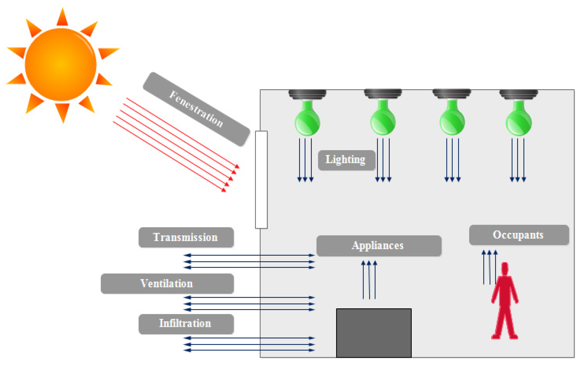
Figure 3.
The program’s main working interface.
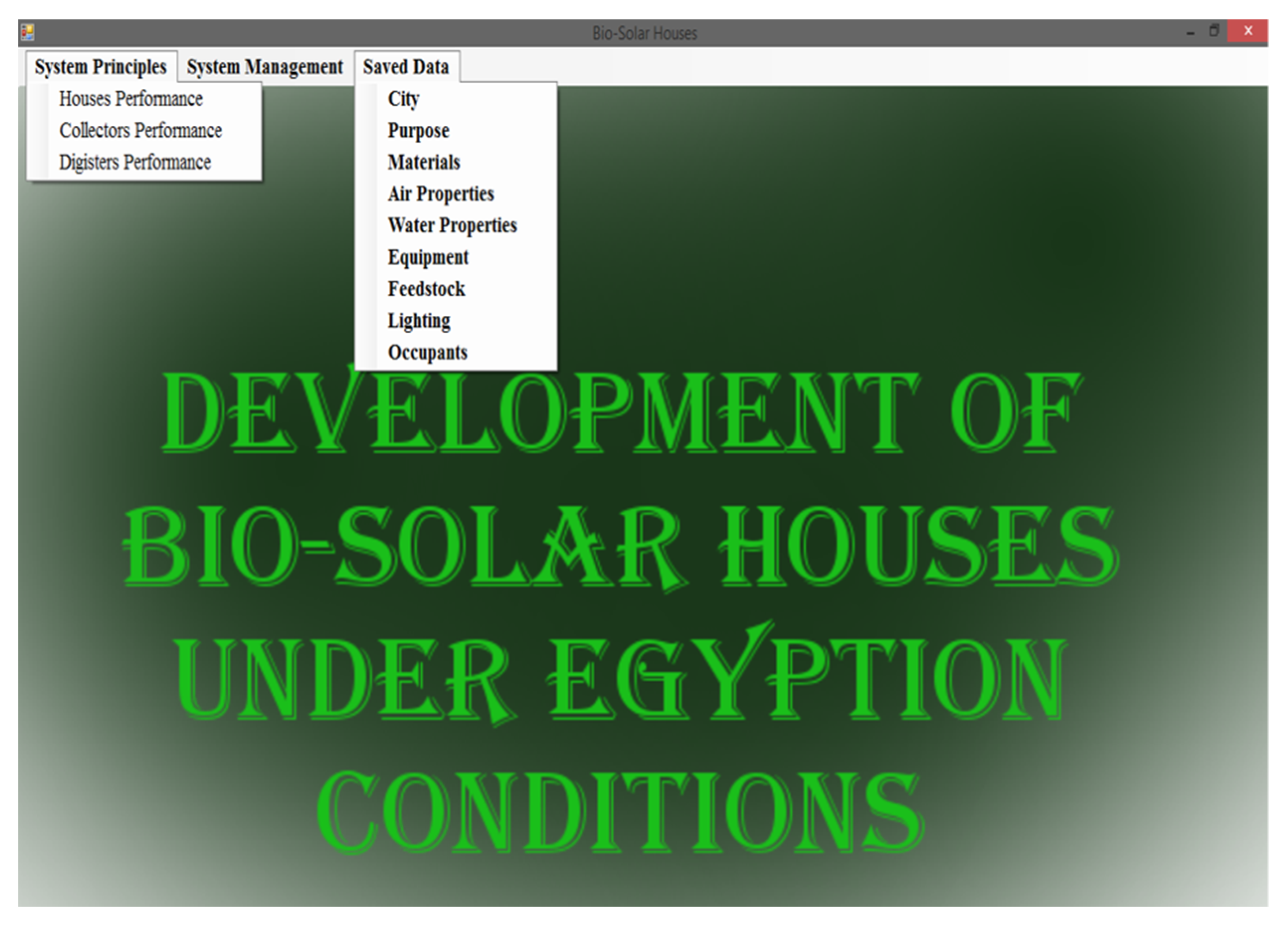
Figure 4.
User approach in the model.
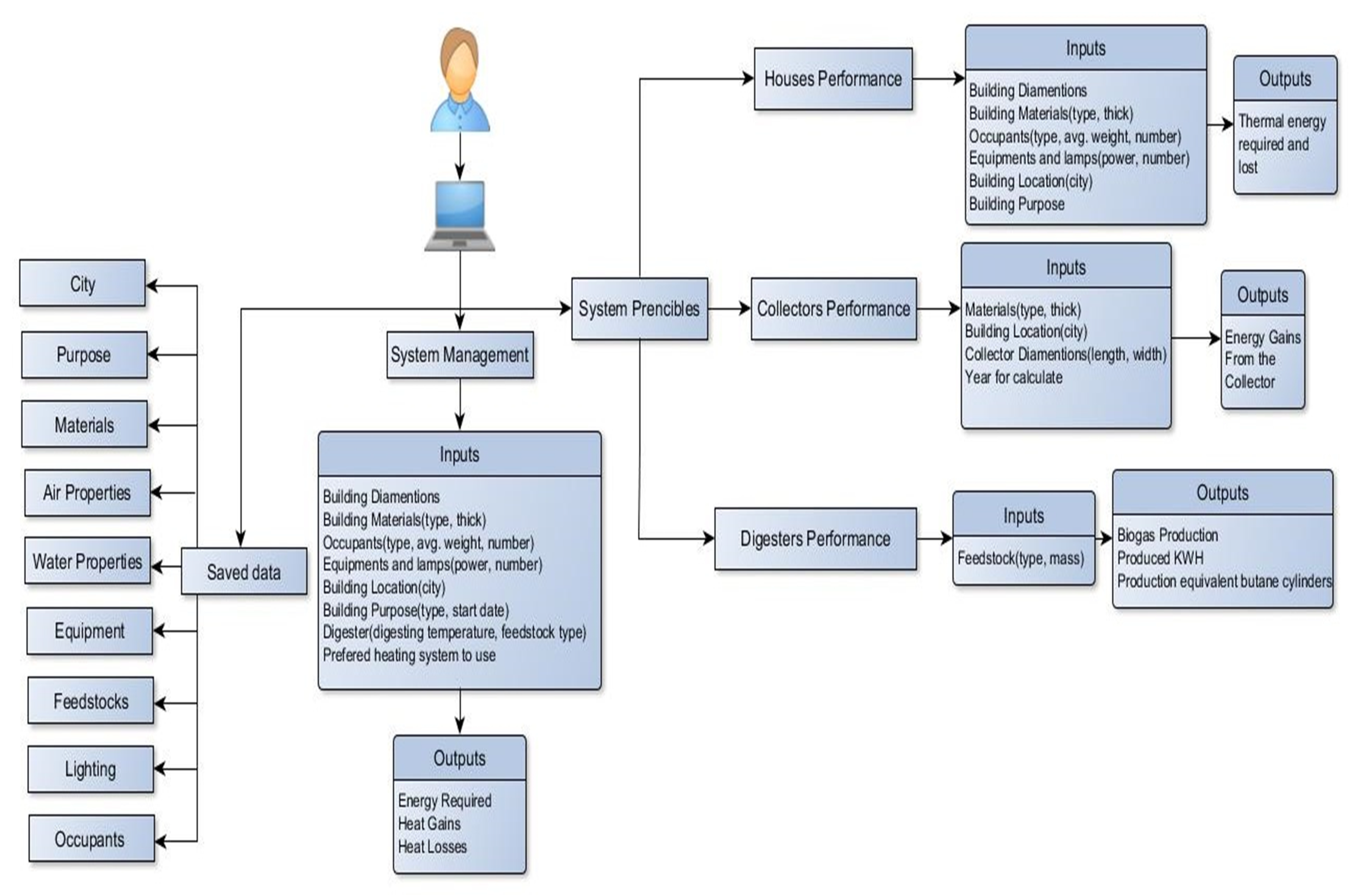
Figure 5.
Houses performance form in model.

Figure 6.
Solar collectors’ form in the model.

Figure 7.
Digesters Performance form in the model.

Figure 8.
System management form in the model.

Figure 9.
Floor plane of single-family detached house.

Figure 10.
Energy requirement for heating and energy gained by solar collector and biogas digester for different bio-solar house case studies during winter season. Case 1. Heating the house with solar energy; Case 2. Heating the house and the biogas digester with solar energy during daylight and with biogas at night (temperature of the biogas digester is 309.15 K and retention time is 35 days); Case 3. Heating the house and biogas digester with solar energy during daylight and with biogas at night (temperature of biogas digester is 322.15 K and retention time is 17.5 days); Case 4. Heating the house with biogas while the biogas digester is heated by solar energy (temperature of biogas digester is 309.15 K and retention time is 35 days); Case 5. Heating the house with biogas while the biogas digester is heated by solar energy (temperature of biogas digester is 322.15 K and retention time is 17.5 days).

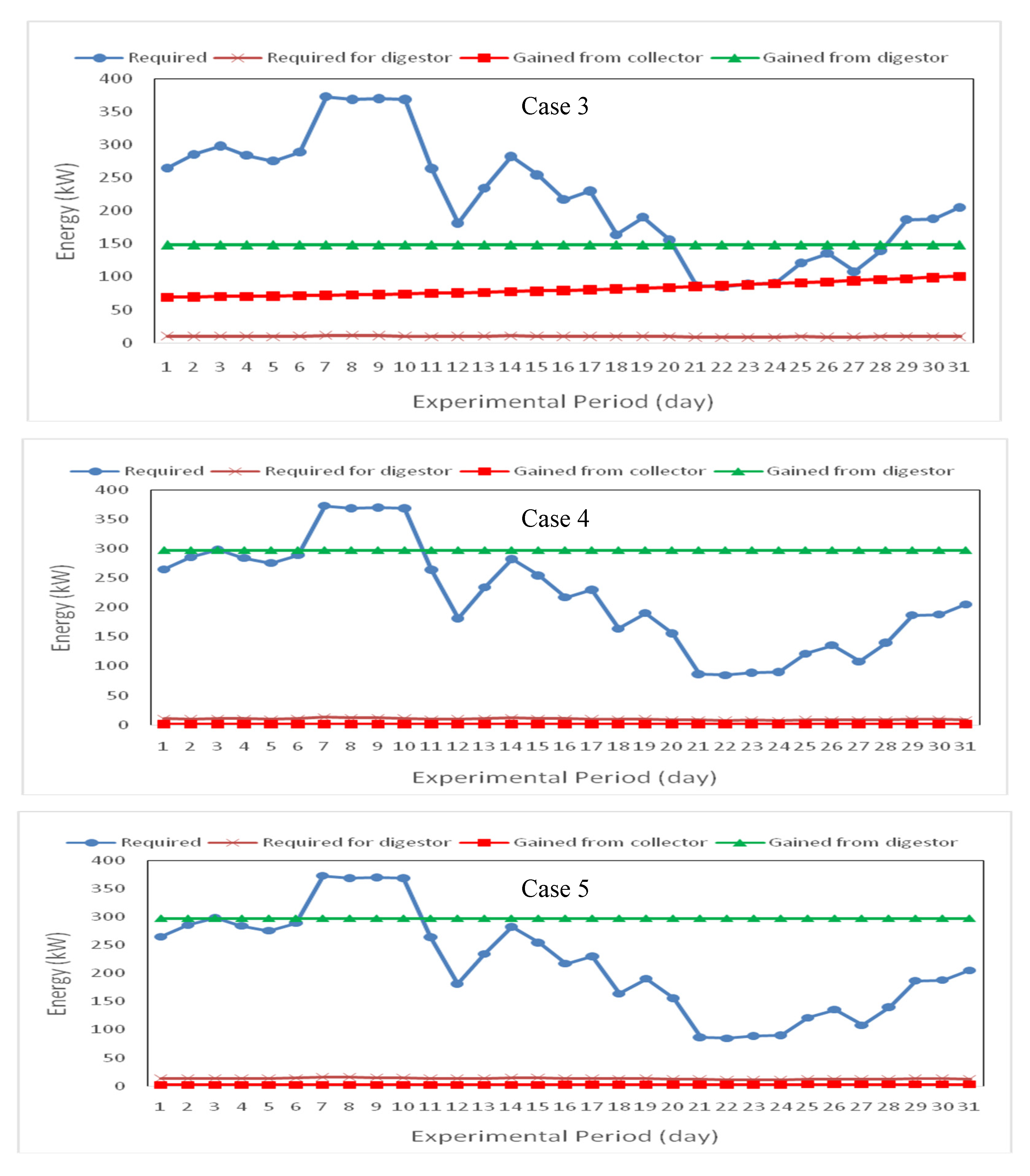
Figure 11.
Energy requirement for cooling and energy gained by solar collector and biogas digester for different bio-solar house during summer season. Case 1. Heating the house with solar energy; Case 2. Heating the house and the biogas digester with solar energy during daylight and with biogas at night (temperature of the biogas digester is 309.15 K and retention time is 35 days); Case 3. Heating the house and biogas digester with solar energy during daylight and with biogas at night (temperature of biogas digester is 322.15 K and retention time is 17.5 days); Case 4. Heating the house with biogas while the biogas digester is heated by solar energy (temperature of biogas digester is 309.15 K and retention time is 35 days); Case 5. Heating the house with biogas while the biogas digester is heated by solar energy


Figure 12.
Biogas production amount based on the use of different wastes.
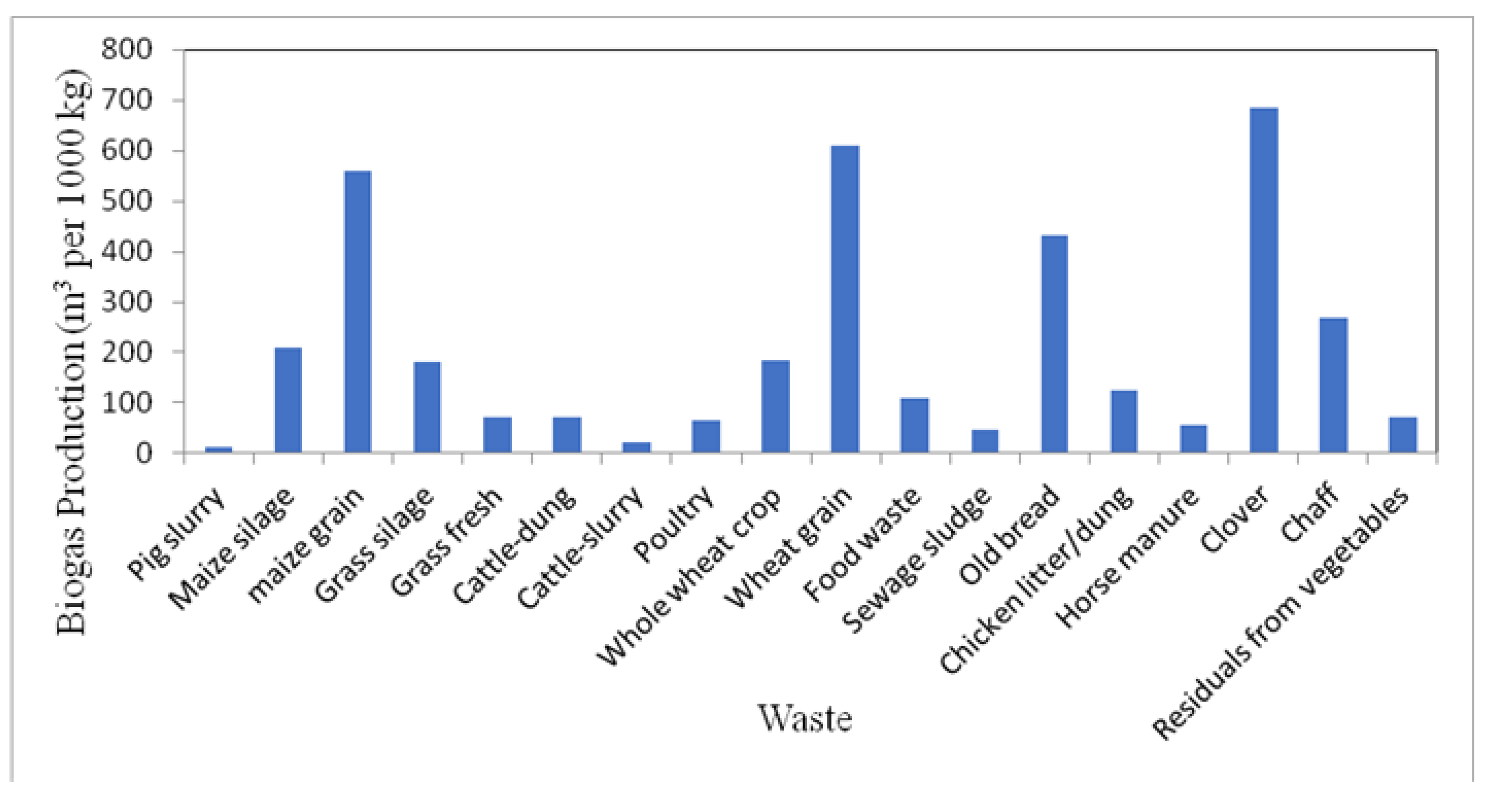
Figure 13.
Heat gained by solar collector during different days over the year.
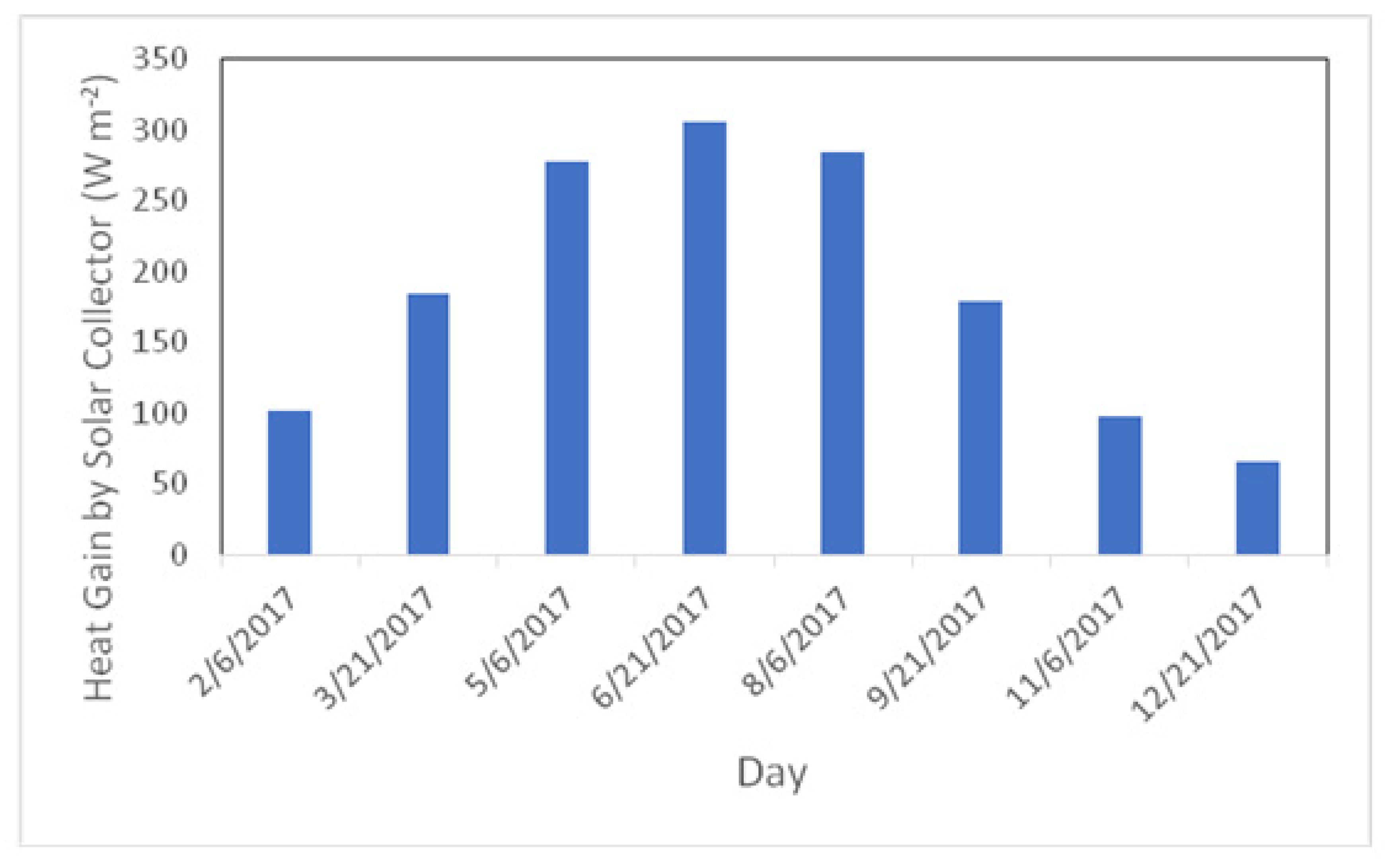
Figure 14.
Predicted and measured energy requirement for heating house during winter season.
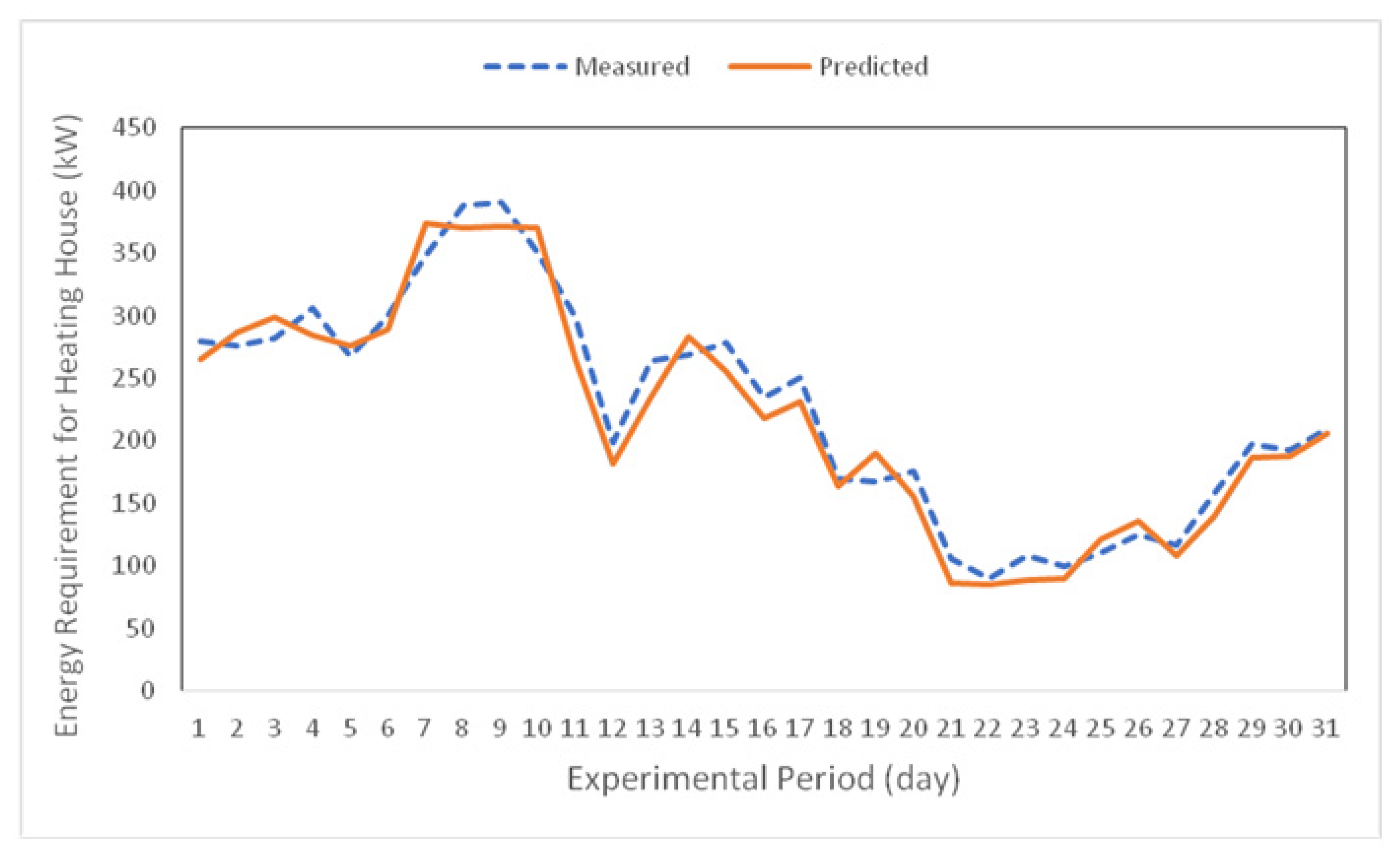
Figure 15.
Comparison between predicted and measured energy requirement for heating the house during winter season.
Figure 15.
Comparison between predicted and measured energy requirement for heating the house during winter season.

Figure 16.
Predicted and measured solar radiation from solar collector.
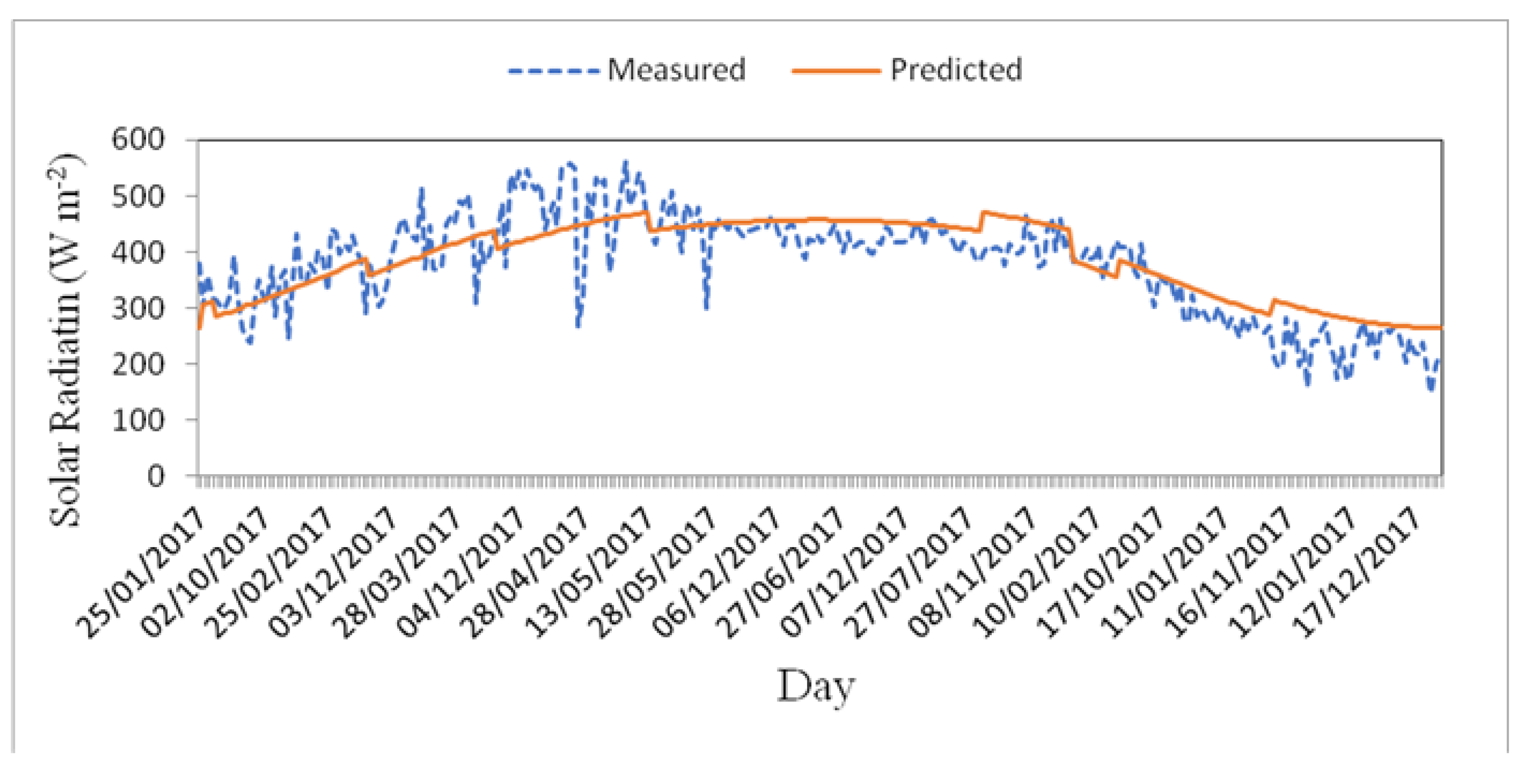
Figure 17.
Comparison between predicted and measured solar radiation.

Figure 18.
Predicted and measured hourly average solar radiation from solar collector.


Table 1.
Parameters used in the energy balance.
| Parameter | Units | Value | Source |
|---|---|---|---|
| V | m s−1 | 0.5 | [17] |
| F | W m−1 K−1 | 1.2 | [17] |
| LSM | Degree | 30 | |
| Ful | - | 1 | |
| Fsa | - | 1 | |
| Hardwoods (K) | W m−1 K−1 | 0.166 | [19] |
| Red brick (K) | W m−1 K−1 | 0.7 | [17] |
| Straw (K) | W m−1 K−1 | 0.042 | [17] |
| Concrete (K) | W m−1 K−1 | 0.93 | [17] |
| Glass (K) | W m−1 K−1 | 1.2 | [17] |
| SHGC | - | 0.25–0.6 | |
| Pg | - | 0.2 | |
| Cn | - | 0.665 | [29] |
| Σ | Degree | 90 |
Table 2.
Specifications of the bio-solar house.
| Type | Material | Material | Thickness (m) |
|---|---|---|---|
| House | Doors | Hardwoods | 0.05 |
| Windows | Glass | 0.006 | |
| Ground | Concrete | 0.1 | |
| Walls | Brick | 0.2 | |
| Straw bales | 0.5 | ||
| Roof | Concrete | 0.1 | |
| Straw bales | 0.5 | ||
| Solar collector | Collector Cover | Glass | 0.01 |
| Absorbent Plate | Black steel | 0.02 | |
| Insulation | Glass wool | 0.05 | |
| Collector Bottom | Black steel | 0.02 | |
| Biogas digester | Digester body | Stainless Steel | 0.02 |
| Foam | 0.05 | ||
| Feedstock | Clover | ||
Table 3.
Data of the used solar collector.
| City | Toukh | |
| Year | 2017 | |
| Tilt angle | 45 | |
| Type | Flat Plate with single cover | |
| Fluid | Air | |
| Collector Dimensions | ||
| Length (m) | Width (m) | |
| 3 | 2 | |
| Collector Materials | ||
| Type | Material | Thick (m) |
| Collector Cover | Glass | 0.01 |
| Absorbent Plate | Black steel | 0.02 |
| Insulation | Glass wool | 0.05 |
| Collector Bottom | Black steel | 0.05 |
Table 4.
The required solar collector area and biogas digester volume for bio-solar house.
| Case | Solar Collector Area, m2 | Biogas Digester Volume, m3 |
|---|---|---|
| First | 177.17 | 9.76 |
| Second | 179.06 | 4.56 |
| Third | 180.31 | 2.28 |
| Fourth | 4.25 | 9.15 |
| Fifth | 8.50 | 4.56 |
© 2020 by the authors. Licensee MDPI, Basel, Switzerland. This article is an open access article distributed under the terms and conditions of the Creative Commons Attribution (CC BY) license (http://creativecommons.org/licenses/by/4.0/).
Share and Cite
MDPI and ACS Style
Khater, E.-S.; Ashour, T.; Ali, S.; Saad, M.; Todic, J.; Hollands, J.; Korjenic, A. Development of a Bio-Solar House Model for Egyptian Conditions. Energies 2020, 13, 817. https://doi.org/10.3390/en13040817
AMA Style
Khater E-S, Ashour T, Ali S, Saad M, Todic J, Hollands J, Korjenic A. Development of a Bio-Solar House Model for Egyptian Conditions. Energies. 2020; 13(4):817. https://doi.org/10.3390/en13040817
Chicago/Turabian StyleKhater, El-Sayed, Taha Ashour, Samir Ali, Manar Saad, Jasna Todic, Jutta Hollands, and Azra Korjenic. 2020. "Development of a Bio-Solar House Model for Egyptian Conditions" Energies 13, no. 4: 817. https://doi.org/10.3390/en13040817
Note that from the first issue of 2016, this journal uses article numbers instead of page numbers. See further details here.