Optimization of Pump Turbine Closing Operation to Minimize Water Hammer and Pulsating Pressures During Load Rejection


1
State Key Laboratory of Water Resources and Hydropower Engineering Science, Wuhan University, Wuhan 430072, China
2
School of Civil, Environmental & Mining Engineering, the University of Adelaide, Adelaide SA 5005, Australia
*
Author to whom correspondence should be addressed.
Energies 2020, 13(4), 1000; https://doi.org/10.3390/en13041000
Submission received: 15 January 2020
/
Revised: 20 February 2020
/
Accepted: 21 February 2020
/
Published: 23 February 2020
(This article belongs to the Special Issue Hydrokinetic Energy Conversion: Technology, Research, and Outlook)
Abstract
:In load rejection transitional processes in pumped-storage plants (PSPs), the process of closing pump turbines, including guide vane (GVCS) and ball valve closing schemes (BVCS), is crucial for controlling pulsating pressures and water hammer. Extreme pressures generated during the load rejection process may result in fatigue damage to turbines, and cracks or even bursts in the penstocks. In this study, the closing schemes for pump turbine guide vanes and ball valves are optimized to minimize water hammer and pulsating pressures. A model is first developed to simulate water hammer pressures and to estimate pulsating pressures at the spiral case and draft tube of a pump turbine. This is combined with genetic algorithms (GA) or non-dominated sorting genetic algorithm II (NSGA-II) to realize single- or multi-objective optimizations. To increase the applicability of the optimized result to different scenarios, the optimization model is further extended by considering two different load-rejection scenarios: full load-rejection of one pump versus two pump turbines, simultaneously. The fuzzy membership degree method provides the best compromise solution for the attained Pareto solutions set in the multi-objective optimization. Employing these optimization models, robust closing schemes can be developed for guide vanes and ball valves under various design requirements.
1. Introduction
In recent years, pumped-storage power plants (PSPs) have become increasingly important in stabilizing and balancing electricity [1,2,3]. They play the roles of frequency regulation, peak shaving, and emergency power supply in a power grid. PSPs are intricate nonlinear systems typically consisting of pipelines, pump turbines, ball valves, reservoirs, and surge tanks. To better present the PSP system in this paper, a basic configuration of a real PSP in China is shown in Figure 1.
To fulfill the above functions, a PSP system has to constantly undergo various transient processes. Load rejection in turbine mode is one of the challenging working conditions threatening the safety of the PSP. When full load rejection occurs, the governor will quickly close the guide vanes. The operating points of pump turbine will go through a so-called reverse-S-shaped region, which may cause a series of instability problems [4,5]. In this case, the water hammer at the spiral case may reach an extremely high level, leading to abnormal vibration and penstock failure, and the pressure at the draft tube may reach an extremely low level, leading to cavitation and even water column separation. Additionally, pulsating pressures, a fluctuation component upon water hammer pressures, may also increase largely when operating in the S-shaped region [6]. The existence of this kind of pressure is one of the main reasons for unit vibration as well as fatigue damage of pump turbines [7,8]. Therefore, minimizing both water hammer and pulsating pressures during load rejection is of great importance to ensure the safety and stability of PSPs.
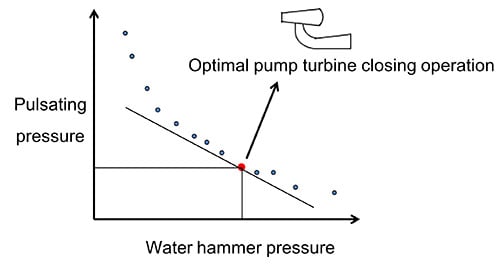
The optimization of guide vane closing schemes (GVCSs) is an important strategy to reduce water hammer pressure and pulsating pressures. Traditionally, a slower guide vane closure means lower water hammer pressure, but a higher rotational speed rise which is often accompanied by larger pulsating pressures. Thus, an optimal GVCS is significant to coordinate the trade-off between them. A lot of research has been done on the GVCS optimization previously. Vakil [9] examined different guide vane closing laws to investigate their effects on pressure rise and speed rise. Zhang et al. [10] introduced a joint closing scheme of guide vane and ball valve in load rejection and indicated that the joint closing scheme can effectively reduce the second pressure peak at the spiral case. Zeng et al. [11] theoretically analyzed the effects of the GVCS on water hammer and pulsating pressures based on the transient characteristics of pump turbines in the S-shaped region.
In addition to those theoretical analyses of the transient process, evolutionary algorithms have also been widely used to seek optimal closing schemes for pump turbines [12,13]. Considering water hammer pressure and speed rise, Zhou et al. [14] solved the GVCS optimization problem using an enhanced multi-objective gravitational search algorithm. Lai et al. [15] conducted the optimization with guide vanes closing in different ways, and they found that the three-stage GVCS achieved better performance in hydraulic transient simulations than the traditional one- or two-stage GVCSs.
Overall, previous studies have done a large number of optimizations based on the evolutionary algorithms using the speed rise and water hammer as objective functions in transient processes, but there is no existing research on optimization for minimizing pulsating pressures of a pump turbine. One reason for this is that it is difficult to model pulsating pressures in one-dimensional flow owing to their obvious three-dimensional characteristics [16,17]. However, as the authors have mentioned above, pulsating pressures control in extreme conditions is necessary, especially when the speed rise within its threshold. Without considering pulsating pressures, the results of previous work may be limited in practical application.
To overcome the shortcomings in existing GVCS optimization, this paper introduces a method of peak-to-peak diagrams [18] into the transient model to estimate dynamic pulsating pressures. The proposed model was then combined with genetic algorithms (GAs) using water hammer and pulsating pressures instead of speed rise as the objective functions. To obtain reliable and applicable closing schemes, both single-objective and multi-objective optimization of GVCS and BVCS are carried out in load rejection in the PSP. The innovations of this research include the following; (1) a method of peak-to-peak diagrams is applied to estimate dynamic pulsating pressures, (2) new objective functions considering water hammer and pulsating pressures are designed to meet different engineering requirements, and (3) both single load rejection and load rejection of two units are incorporated within the optimization model to broaden the applicability of the optimized results.
The remainder of this article is organized as follows. Section 2 constructs the hydraulic transient model, including the method to estimate dynamic pulsating pressures. Section 3 describes the formulation for optimizing the pump turbine closing operation by means of evolutionary algorithms. In Section 4, the transient model is validated with field test results. Then, three cases are carried out to optimize the pump turbine closing operation and the results are presented with the corresponding analyses. Section 5 summarizes the main results and presents conclusions.
2. Hydraulic Transient Simulation with Pulsating Pressure Estimation
Figure 1 shows a typical kind of PSP system with two pump turbines sharing the same main pipelines. To ensure the safe and reliable operation of the pump turbine, the inlet of each pump turbine is equipped with a ball valve. Based on the actual installation, two surge tanks are adopted to control transient in this system.
In this section, the hydraulic transient model based on the method of characteristics (MOC) is first established to calculate water hammer pressure. The models of pipeline system, pump turbine, and ball valve are briefly introduced, and more detailed information can also be found in the literature [19,20,21]. Then a method of peak-to-peak diagrams is proposed to estimate pulsating pressures.
2.1. Pipeline System Model
In the case of unsteady compressible liquid flow in elastic pressurized pipelines, governing equations can be considered as
where is the piezometric head, is flow velocity, is the distance along the pipeline, and is time; is wave speed, is gravitational acceleration, is the pipe diameter, and is the Darcy–Weisbach friction factor.
To solve the above partial differential equations, the method of characteristics described in [22] is employed as the numerical method for the pipeline system. This method, in essence, transforms Equations (1) and (2) into an ordinary differential equation set in the range of the characteristic lines. Along the right line and left line (Figure 2), the flow and head in the pipelines satisfy Equations (3) and (4):
where is the flow rate. Therefore, the finite difference method can be used to obtain Equations (5) and (6) for unknown and
2.2. Pump Turbine Model
In this paper, a validated pump turbine model presented in [19] is introduced based on its characteristic curves. In this case, the flow function and torque function are described by flow characteristic curves (in Figure 3a) and torque characteristic curves (Figure 3b). Consequently, the mathematical model of pump turbine can be written as
where and denote the interpolation functions between flow characteristic curves and torque characteristic curves, respectively, with the guide vane opening y (GVO) and the unit rotational speed as the inputs; and represent the unit flow and unit torque, respectively; is rotational speed, and and are the flow rate and the torque of the pump turbine, respectively; is the inlet diameter of the runner is the water head, is the generator moment of inertia, and is the load moment, which is equal to 0 in load rejection.
Figure 3 shows a part of the characteristic curves which were provided by the manufacturer through model tests. However, the characteristic curves exhibit a reverse “S” shape, crossover, and overlap between each other (as shown in the ellipses in Figure 3), which may cause multi-value problems in the interpolation. Thus, an improved Suter transformation method in [23] is employed to exact the uneven characteristic curves.
2.3. Ball Valve Model
The ball valve should also be closed immediately in case of an emergency shutdown of the unit to ensure that the pulsating pressure does not exceed the specified value. The mathematical model of ball valve is
where is the flow of ball valve; and is the coefficient of flow and area of ball valve opening (BVO), respectively; and is the head difference between upstream and downstream of the ball valve. In practice, the function is normally considered as a parameter changing with BVO.
2.4. Estimating Dynamic Pulsating Pressures
The above hydraulic transient model is capable of calculating water hammer pressures, but not of calculating pulsating pressures. Thus, this paper applied a method of peak–peak diagrams into the transient model for estimating pulsating pressures.
Figure 4 shows the used peak–peak diagrams provided by the manufacturer. They demonstrate the contours of the pulsating pressures in the spiral case (Figure 4a) and in the draft tube (Figure 4b) of the pump turbine. Each contour line corresponds to a specific relative amplitude of pulsating pressure. The amplitude of the pulsating pressures increases in the turbine‘s working region, reaching its maximum around the runaway curve.
Based on the peak-to-peak diagrams, the estimation of pulsating pressures can be divided into three stages:
(1) Extension of contour lines
The data of pulsating pressure in pump turbine model tests usually include only the turbine operation area, but the operating points of load rejection have to experience braking region (from runaway to zero flow) and reverse-pumping region (after zero flow). To obtain the pulsating pressure contour map of the above region, the contour lines are extended according to its distribution and trend. Figure 5 gives the extended contour lines.
(2) Interpolation of the relative amplitude of pulsating pressure
Then, by plotting the operational trajectory on the peak-to-peak diagrams, the relative amplitude of pulsating pressure for each operating point can be interpolated. The relative amplitude of pulsating pressure is expressed as
where is the relative amplitude of pulsating pressure and is the function of interpolation. In this paper, the interpolation algorithm in map design [24] is adopted for .
(3) Calculation of pulsating pressure magnitude
Finally, transforming the relative amplitude into absolute magnitude by Equation (10), the magnitude variation of pulsating pressures can then be estimated.
where is the pulsating pressure magnitude, which is half the peak-to-peak value, and is the water head of the pump turbine. Figure 6 shows the architecture of pulsating pressure estimation based on peak-peak diagrams.
3. Formulations for Optimization of Pump Turbine Closing Process
Based on the hydraulic transient model, both the genetic algorithm (GA) and non-dominated sorting genetic algorithm (NSGA-II) are employed to optimize GVCS and BVCS in load rejection. Single-objective [25,26] and multi-objective optimization cases [12,14,27] are considered to meet various engineering requirements. The water hammer and pulsating pressures are synthesized into the total dynamic pressure in the single-objective optimization. In comparison, the multi-objective optimization leads to a set of Pareto non-dominated solutions that can give the operator more flexible choices according to the actual onsite conditions.
3.1. Closing Strategies
Multiple closing strategies are considered in this study, including two-stage GVCS, three-stage GVCS, and GVCS combined with BVCS. Schematics of the two-stage and three-stage GVCSs are shown in Figure 7, with BVCS only adopting the two-stage scheme.
The initial opening and the total closing time of valves are set to be constants. Therefore, the decision variables can be defined by the coordinates of inflection points. According to the closing strategies, the decision vectors are formulated as (1) two-stage GVCS, ; (2) three-stage GVCS, ; (3) two-stage GVCS with BVCS, ; and (4) three-stage GVCS with BVCS, , where and are the abscissa and ordinate of the first inflection point of the guide vane closing curve, and are the abscissa and ordinate of the second inflection point of the guide vane closing curve, and and are the abscissa and ordinate of the inflection point of the ball valve closing curve.
3.2. Objective Functions
When designing PSPs, the total dynamic pressures at the inlet of the spiral case and the outlet of the draft tube during load-rejection scenarios are crucial. The maximum pressure at the spiral case determines the required structural strength of the pipelines, and the minimum pressure at the draft tube needs to exceed the vapor pressure in order to avoid separation of the fluid column, which may generate a huge pressure surge in the draft tube. Thus, the first objective function considers the total dynamic pressures and is defined as
where and are the water hammer pressures at the spiral case and draft tube, respectively, and and are the magnitudes of the corresponding pulsating pressures. Term is defined as the simulated dynamic pressure envelop at the spiral case, and term is defined as the simulated dynamic pressure envelop at the draft tube.
Using Equation (11) as the objective function, the optimized GVCS and BVCS may not be sufficiently robust or suitable for other scenarios. To address this issue and increase the applicability of the optimized results, multiple scenarios can be considered simultaneously during the optimization process. Therefore, another objective function incorporating multiple scenarios is defined as
where the subscript represents the parameters for scenario , N is the total number of scenarios, and is the weighting coefficient that can be varied for different PSPs. Therefore, the user can choose different weights according to the security level of different scenarios.
Pulsating pressure is a major consideration for turbine manufacturers. Thus, optimization of water hammer pressures and pulsating pressures need to be sometimes separated. Typically, pulsating pressure is greatest at the vaneless space, and that in the draft tube can cause cavitation and affect the operational stability of the pump turbine. Because the peak-to-peak pulsating pressure diagram at the vaneless space is not available, the pulsating pressure at the spiral case, which is mostly propagated from the vaneless space, is used instead to assess the detrimental effects on the turbine. Thus, the other two objective functions can be defined as
where and are weighting coefficients.
3.3. Constraints
Multiple constraints are considered in the optimization process, to accelerate the convergence and to improve the search efficiency.
(1) Limit of the closing rate
The relative closing rates of guide vanes and ball valves can be illustrated as Equation (15).
In Equation (15), and are the closing rates of guide vanes and ball valves, respectively, and and represent the maximum limits of the two kinds of closing rates.
(2) Limit of closing time
In the actual load-rejection process, the total closing time of the guide vanes is limited to a range that can be described as
where is the total closing time of the guide vanes, and and are the minimum and maximum closing times of the guide vanes, respectively.
The closing time of the ball valve is longer than that of the guide vanes, and thus
where is the total closing time of the ball valve and is the corresponding maximum closing time.
(3) Limit of transient pressures at the spiral case and ball valve
The simulated transient pressure at the spiral case should be limited to a certain level in order to meet the PSP design requirements. Considering the simulation error, a 10% margin for pressure rise is considered, and the constraint on pressure rise is defined as
where is the initial pressure at the spiral case and is the maximum transient pressure allowed at the spiral case.
BVCS might take the risks of displacement and shortened service life of the ball valve in a real system because of the pressure differences between inlet and outlet. Therefore, the inlet pressure of the ball valve should also be monitored [28]. The inlet pressure constraint of the ball valve is set to be the same as that of the spiral case.
(4) Limit of transient pressure at the draft tube
Similar to the pressure constraint at the spiral case, the constraint of transient pressure at the draft tube is set as
where is the initial pressure at the draft tube and is the minimum transient pressure allowed at the draft tube.
(5) Constraints on the water level in surge tanks
The water levels in a surge tank are constrained as
where is the water level present in the surge tank, and and are the minimum and maximum allowable water levels in the surge tank.
(6) Limit on the rate of speed rise
The constraint of the rate of speed rise is given by
where is the maximum rotational speed during the transient process, is the rated rotational speed, and is the maximum relative speed rise.
(7) Limit on rotational speed oscillation
The number of rotational speed oscillations is constrained as
3.4. Evolutionary Algorithms
(a) Genetic algorithm
GAs are popular in engineering [29]. In a GA, each individual within a population is a feasible solution in the solution space. By simulating the evolution process of organisms, the optimal solution is searched for in the solution space. Compared with other optimization methods, a GA has advantages such as strong adaptability, global optimization, simplicity, and universality. Therefore, GAs were adopted for optimization in this paper.
(b) NSGA-II and fuzzy membership degree method
The process of closing pump turbines is fundamentally a multi-objective optimization problem involving multiple constraints because the water hammer pressure and pulsating pressure are conflicting. The Pareto-based NSGA-II [30], one of the most popular multi-objective evolutionary algorithms, has been used in a wide range of multi-objective problems owing to its simple and efficient non-dominated ranking procedure for yielding different Pareto frontier levels. Thus, it is adopted here to optimize the pump turbine closing operation.
The Pareto frontiers provide a set of optimal solutions, from which the most compatible solution can be selected. The fuzzy membership degree method [13] is applied to make fuzzy evaluations for each solution and can be described for each objective function by
where is the value of the kth objective function, with the subscripts and indicating the maximum and minimum values of the corresponding objective function, respectively. The best compatible solution is that with the maximum , which is defined as
where is the number of objective functions to be optimized.
4. Results and Discussion
4.1. System Specification of the PSP and Field Tests
The case studies presented here are associated with a real PSP in China, with two pump turbines sharing the same main pipelines as shown in Figure 1. The basic parameters of this PSP are listed in Table 1. Some operational requirements that guarantee the safety of the PSP during load-rejection scenarios are listed in Table 2.
A field test of load rejection for a single pump turbine was conducted by the turbine manufacturer. The flow was regulated by both guide vanes and the ball valve, with the GVCS and BVCS shown in Figure 8. The load rejection transient process began at 2.96 s. After a short delay, the guide vanes were stalled for approximately 2.98 s, and then fully closed at t = 30.09 s. The ball valve was closed with the closing speed changed at t = 37.65 s.
The same load rejection process was carried out using the proposed model in this paper. The characteristic curves of the pump turbine are shown in Figure 3. The peak-to-peak pulsating pressure diagrams from model tests are shown in Figure 5. The measured and simulated rotational speeds are shown in Figure 9. The measured pressures are shown in Figure 10. It is important to note that the black lines in Figure 10 are the measured total pressure, whereas the red lines are the simulated total pressure envelopes, comprised of the simulated water hammer pressure (in blue lines) and the magnitude of the estimated pulsating pressure.
It can be seen from Figure 9 and Figure 10 that the predicted results are in good agreement with the field data. During the first 8 seconds, the predicted rotational speed first increased and reached its maximum value of 129%, nearly 1 second ahead of the occurring time of the measured maximum of 132%. Then, it dropped sharply. At ~18 s, the rotational speed reached its second maximum of 109%, which was the same as the measured data. The predicted and measured pressures at the spiral case showed a similar tendency with the rotational speed change while the pressure trace at the draft tube appeared inversely as expected. The extremums of the measured and predicted total pressures at the spiral case are 739.1 m and 734.3 m. The extremums of the measured and predicted total pressure at the draft tube are 49.1 m and 51.6 m. To better present the comparison, the measured and predicted extremums and absolute errors are listed in Table 3.
Considering the errors in the characteristic curves between the real and model pump turbines, together with uncertainties in the field tests and some other error sources, it can be concluded that the numerical model achieves good accuracy in simulating water hammer pressure, and is capable of predicting the changing trend in pulsating pressures during load-rejection scenarios.
In the following sections, three optimization cases are discussed. In Case 1 (single-objective optimization), the guide vanes of one pump turbine are closed in either two or three stages, and the other pump turbine is always closed (the scenario is defined as a single load-rejection scenario). Case 2 (single-objective optimization) considers two load-rejection scenarios: the single load-rejection scenario and the simultaneous load-rejection of two pump turbines. In Case 3, multi-objective optimization of two load-rejection scenarios was conducted by separating the water hammer pressure and the pulsating pressure in the objective functions.
4.2. Case 1: Single-Objective Optimization of Single Load Rejection Scenario
The load rejection start time was set at 0 s. The total closing times of the guide vanes and the ball valve were set to 26 s and 35 s, respectively, which are consistent with the field tests. These settings are consistent in all of the following cases. Other optimization constraints are described in the previous section and Table 2. The GA parameters were set as follows; , , , , , where is the total generation, is the population size, is the probability of crossover, is the probability of mutation, and is the percentage of genetic mutation. The objective function is defined in Equation (11).
Four subcases (Cases 1.1–1.4) in Table 4 are considered in this section. By running the optimization model, the variations in the objection function across multiple iterations were obtained, as shown in Figure 11; the optimized closing schemes are shown in Figure 12.
It can be seen in Figure 12 that the optimized GVCSs are similar to the theoretical schemes derived in [11]. Comparing cases 1.1 and 1.2 in Figure 13 and Figure 14, respectively, the three-stage closing scheme leads to better performance in terms of both transient pressure and rotational speed. The pressure traces at the spiral case show two peaks for both cases, and increasing the number of closing stages from two to three markedly reduces the first pressure peak when comparing Case 1.1 with Case 1.2 or Case 1.3 with Case 1.4.
4.3. Case 2: Single-Objective Optimization of Two Load Rejection Scenarios
In Case 2, multiple load-rejection scenarios were taken into the single-objective optimization to find a robust closing scheme. The first scenario (Scenario 1) was a single load rejection scenario, and the other (Scenario 2) scenario was a simultaneous full load rejection of two units.
Scenarios 1 and 2 shared a common three-stage GVCS with BVCS in this case. The constraints and setting parameters matched those in Case 1.4. The objective function with N = 2 (in Equation (12)) was used for the optimization. In a real PSP system, Scenario 2 is more hazardous than Scenario 1. Thus, a larger weighting factor was assigned to 0.7, which means giving more emphasis on Scenario 2. The weighting factor for Scenario 1 was correspondingly assigned to 0.3.
The optimized three-stage GVCS with BVCS is shown in Figure 15, and the dynamic pressure envelopes of the two scenarios are shown in Figure 16. Because the pipeline system is symmetrical with two identical units, only the transient pressure in Unit 2 is presented in Scenario 2 in Figure 16. By comparing the optimized closing schemes with those in Case 1.4, it was found that the optimized GVCS has the same pattern and slightly different turning positions. Thus, such “closing-stall-closing” GVCS is robust for different load-rejection scenarios.
4.4. Case 3: Multi-Objective Optimization of Two Load Rejection Scenarios
In this case, the objective function for water hammer pressures and objective function for pulsating pressures were optimized simultaneously in NSGA-II. The same two scenarios and weighting factors that used in Case 2 were considered in and . As NSGA-II is a multi-objective optimization genetic algorithm, the control parameters are mostly the same as those of the GA in Case 1. However, a larger population size was used (np = 50) in order to maintain the diversity of solutions as far as possible.
Two subcases were considered in the optimization with (1) guide vanes closed in two stages (Case 3.1) or three stages (Case 3.2), and (2) ball valves closed for both cases.
By running the optimization model, the Pareto front plots were obtained as shown in Figure 17, and the fuzzy membership degree of each Pareto solution was then calculated using Equations (23) and (24). The objective function values as well as the values of partial Pareto-optimal sets are partially given in Table 5.
Finally, Scheme 44 in Case 3.1 and Scheme 43 in Case 3.2, which have the maximum value of , were selected out for the analysis. The optimized closing schemes are shown in Figure 18.
Figure 17 shows that the selected schemes give more emphasis on reducing the pulsating pressures. Thus, similar GVCSs are obtained for the first 5 s, in which the water hammer pressures increase to their maximum. The GVCSs after 5 s do not affect the maximum transient pressures, as shown in Figure 19 and Figure 20, and thus the two-stage closing scheme is sufficient to achieve adequate results. If the water hammer pressures are assigned a higher priority in the design process, then the weighting factors and in Equation (13) can be increased.
5. Conclusions
In this paper, a transient model of load rejection was developed to simulate water hammer pressures and to estimate pulsating pressures in pump turbines. The numerical model was validated by field tests and was then combined with evolutionary algorithms to optimize the pump turbine closing operations (i.e., GVCS and BVCS). By conducting three optimization cases, robust, reliable, and adaptable pump turbine closing operations were obtained for different engineering requirements.
The optimized results have indicated that (1) pressure factors in the pump turbine can be reduced by using GA (for total dynamic pressures) and NSGA-II (for water hammer and pulsating pressures), (2) the three-stage GVCSs are more effective in diminishing the first pressure peak seen on total transient pressure traces when compared with two-stage GVCSs, and (3) such “closing-stall-closing” three-stage GVCSs are applicable to multiple load-rejection scenarios. Overall, this work provided new insight for reducing pulsating pressures in PSPs. However, the estimated pulsating pressures in the proposed model may include some deviation due to the error of peak-to-peak diagrams. Further work will be conducted to improve the estimation performance with the assistance of field tests.
Author Contributions
J.Y. (Jiawei Ye) built the model, performed the simulations and calculations and wrote the paper. W.Z. contributed with discussions, ideas and valuable insights. Z.Z. and J.Y. (Jiandong Yang) revised the paper; J.Y. (Jiebin Yang) proposed the theory. All authors have read and agreed to the published version of the manuscript.
Funding
The research presented in this study was supported by the Open Research Fund Program of State Key Laboratory of Water Resources and Hydropower Engineering Science (Grant 2017SDG01). This work was also supported by the National Natural Science Foundation of China (NSFC) (Nos. 51879200, No.51809197).
Conflicts of Interest
The authors declare no conflict of interest.
References
- Rehman, S.; Al-Hadhrami, L.M.; Alam, M.M. Pumped hydro energy storage system: A technological review. Renew. Sust. Energy Rev. 2015, 44, 5865–5898. [Google Scholar] [CrossRef]
- Mitchell, C. Momentum is increasing towards a flexible electricity system based on renewables. Nat. Energy 2016, 1, 15030. [Google Scholar] [CrossRef]
- Chazarra, M.; Pérez-Díaz, J.I.; García-González, J.; Praus, R. Economic viability of pumped-storage power plants participating in the secondary regulation service. Appl. Energy 2018, 216, 224–233. [Google Scholar] [CrossRef]
- Cavazzini, G.; Covi, A.; Pavesi, G.; Ardizzon, G. Analysis of the unstable behavior of a pump-turbine in turbine mode: Fluid-dynamical and spectral characterization of the S-shape characteristic. J. Fluids Eng. Trans. ASME 2015, 138, 021105. [Google Scholar] [CrossRef]
- Zeng, W.; Yang, J.; Guo, W. Runaway instability of pump-turbines in S-shaped regions considering water compressibility. J. Fluids Eng. Trans. ASME 2015, 137, 051401. [Google Scholar] [CrossRef]
- Wang, Z.; Zhu, B.; Wang, X.; Qin, D. Pressure Fluctuations in the S-Shaped Region of a Reversible Pump-Turbine. Energies 2017, 10, 96. [Google Scholar] [CrossRef] [Green Version]
- Zuo, Z.; Fan, H.; Liu, S.; Wu, Y. S-shaped characteristics on the performance curves of pump-turbines in turbine mode—A review. Renew. Sust. Energy Rev. 2016, 60, 836–851. [Google Scholar] [CrossRef]
- Tanaka, H. Vibration Behavior and Dynamic Stress of Runners of Very High Head Reversible Pump-turbines. Int. J. Fluid Mach. Syst. 2011, 4, 289–306. [Google Scholar] [CrossRef]
- Vakil, A.; Firoozabadi, B. Investigation of Valve-Closing Law on the Maximum Head Rise of a Hydropower Plant. Sci. Iran. Trans. B Mech. Eng. 2009, 16, 2222–2228. [Google Scholar]
- Zhang, C.; Yang, J. Study on Linkage Closing Rule between Ball Valve and Guide Vane in High Head Pumped Storage Power Station. Water Resour. Power 2011, 29, 128–131. [Google Scholar]
- Zeng, W.; Yang, J.; Hu, J.; Yang, J. Guide-Vane Closing Schemes for Pump-Turbines Based on Transient Characteristics in S-shaped Region. J. Fluids Eng. 2016, 138, 051302. [Google Scholar] [CrossRef]
- Zhao, Z.; Yang, J.; Yang, W.; Hu, J.; Chen, M. A coordinated optimization framework for flexible operation of pumped storage hydropower system: Nonlinear modeling, strategy optimization and decision making. Energy Convers. Manag. 2019, 194, 75–93. [Google Scholar] [CrossRef]
- Zhou, J.; Wu, Y.; Xu, Y.; Zheng, Y. Research on optimization method of pumped-storage units guide vane closing law. J. Huazhong Univ. Sci. Technol. (Nat. Sci. Ed.) 2017, 45, 123–127. [Google Scholar]
- Zhou, J.; Xu, Y.; Zheng, Y.; Zhang, Y. Optimization of guide vane closing schemes of pumped storage hydro unit using an enhanced multi-objective gravitational search algorithm. Energies 2017, 10, 911. [Google Scholar] [CrossRef]
- Lai, X.; Li, C.; Zhou, J.; Zhang, N. Multi-objective optimization of the closure law of guide vanes for pumped storage units. Renew. Energy 2019, 139, 302–312. [Google Scholar] [CrossRef]
- Xia, L.; Cheng, Y.; Cai, F. Pressure Pulsation Characteristics of a Model Pump-turbine Operating in the S-shaped Region: CFD Simulations. Int. J. Fluid Mach. Syst. 2017, 10, 2872–2895. [Google Scholar] [CrossRef] [Green Version]
- Hu, J.; Yang, J.; Zeng, W.; Yang, J. Transient Pressure Analysis of a Prototype Pump Turbine: Field Tests and Simulation. J. Fluids Eng. 2018, 140, 071102. [Google Scholar] [CrossRef]
- Yang, J.; Yang, J.; Wang, C.; Bao, H. Simulation of pressure fluctuation of a pump turbine in load rejection. J. Hyroelectr. Eng. 2014, 33, 2862–2894. [Google Scholar]
- Chaudhry, M.H. Applied Hydraulic Transients; Springer: New York, NY, USA, 2014. [Google Scholar]
- Li, X.; Tang, X.; Shi, X.; Chen, H.; Li, C. Load rejection transient with joint closing law of ball-valve and guide vane for two units in pumped storage power station. J. Hydroinf. 2017, 20, 3013–3015. [Google Scholar] [CrossRef] [Green Version]
- Journal of Fluids EngineeringWylie, E.B.; Streeter, V.L.; Suo, L. Fluid Transients in Systems; Prentice-Hall: Englewood Cliffs, NJ, USA, 1993. [Google Scholar]
- Karney, B.W.; Ghidaoui, M.S. Flexible discretization algorithm for fixed-grid MOC in pipelines. J. Hydraul. Eng. 1997, 123, 1004–1011. [Google Scholar] [CrossRef]
- Zhou, J.; Zhao, Z.; Zhang, C.; Li, C.; Xu, Y. A real-time accurate model and its predictive fuzzy PID controller for pumped storage unit via error compensation. Energies 2017, 11, 35. [Google Scholar] [CrossRef] [Green Version]
- Hu, W.; Wu, B.; Ling, H. An Automatic Method for Contour Interpolation in Map Design. Available online: http://en.cnki.com.cn/Article_en/CJFDTotal-JSJX200008010.htm (accessed on 23 February 2020).
- Mousavi, S.J.; Shourian, M. Capacity optimization of hydropower storage projects using particle swarm optimization algorithm. J. Hydroinf. 2009, 12, 2752–2791. [Google Scholar] [CrossRef]
- Fu, W.; Tan, J.; Zhang, X.; Chen, T.; Wang, K. Blind Parameter Identification of MAR Model and Mutation Hybrid GWO-SCA Optimized SVM for Fault Diagnosis of Rotating Machinery. Complexity 2019, 2019, 17. [Google Scholar] [CrossRef]
- Li, F.-F.; Qiu, J. Incorporating ecological adaptation in a multi-objective optimization for the Three Gorges Reservoir. J. Hydroinf. 2015, 18, 5645–5678. [Google Scholar] [CrossRef]
- Meniconi, S.; Brunone, B.; Mazzetti, E.; Laucelli, D.B.; Borta, G. Hydraulic characterization and transient response of pressure reducing valves: Laboratory experiments. J. Hydroinf. 2017, 19, 798–810. [Google Scholar] [CrossRef]
- Boeringer, D.W.; Werner, D.H. Particle swarm optimization versus genetic algorithms for phased array synthesis. IEEE Trans. Antennas Propag. 2004, 52, 7717–7779. [Google Scholar] [CrossRef]
- Deb, K.; Pratap, A.; Agarwal, S.; Meyarivan, T. A fast and elitist multiobjective genetic algorithm: NSGA-II. IEEE Trans. Evol. Comput. 2002, 6, 1821–1897. [Google Scholar] [CrossRef] [Green Version]
Figure 1.
Basic configuration of a pumped-storage plant (PSP) with two pump turbines sharing the same main pipelines.
Figure 1.
Basic configuration of a pumped-storage plant (PSP) with two pump turbines sharing the same main pipelines.

Figure 2.
Difference mesh for the method of characteristic.

Figure 3.
Characteristic curves of pump turbine: (a) flow–speed and (b) torque–speed.

Figure 4.
Peak-to-peak diagrams of pulsating pressures in a model pump turbine at (a) the spiral case and (b) the draft tube.
Figure 4.
Peak-to-peak diagrams of pulsating pressures in a model pump turbine at (a) the spiral case and (b) the draft tube.

Figure 5.
Extended peak-to-peak diagrams of the pulsating pressures in a model pump turbine at (a) the spiral case and (b) the draft tube.
Figure 5.
Extended peak-to-peak diagrams of the pulsating pressures in a model pump turbine at (a) the spiral case and (b) the draft tube.

Figure 6.
Process of pulsating pressure estimation.

Figure 7.
Closing operation of a PSP with (a) a two-stage guide vane closing scheme (GVCS) and (b) a three-stage GVCS.
Figure 7.
Closing operation of a PSP with (a) a two-stage guide vane closing scheme (GVCS) and (b) a three-stage GVCS.

Figure 8.
GVCS and ball valve closing schemes (BVCS) in the field test.

Figure 9.
Comparison of measured and simulated rotational speeds.

Figure 10.
Comparison of measured and simulated pressures at (a) spiral case and (b) draft tube.

Figure 11.
Objective function variations with the number of iterations (Case 1).

Figure 12.
Optimized closing schemes in Case 1 for (a) guide vanes and (b) ball valve.

Figure 13.
Comparison of rotational speeds between subcases in Case 1.

Figure 14.
Comparison of dynamic pressure envelopes between subcases in Case 1 at (a) the spiral case and (b) the draft tube.
Figure 14.
Comparison of dynamic pressure envelopes between subcases in Case 1 at (a) the spiral case and (b) the draft tube.

Figure 15.
Comparison of optimized closing schemes between subcases in Case 2.

Figure 16.
Comparison of dynamic pressure envelopes between the two scenarios in Case 2 at (a) the spiral case and (b) the draft tube.
Figure 16.
Comparison of dynamic pressure envelopes between the two scenarios in Case 2 at (a) the spiral case and (b) the draft tube.

Figure 17.
Pareto fronts obtained by different guide vane closing schemes in Case 3.

Figure 18.
Comparison of optimized closing schemes in Case 3 for (a) guide vanes and (b) ball valve.
Figure 18.
Comparison of optimized closing schemes in Case 3 for (a) guide vanes and (b) ball valve.

Figure 19.
Comparison of water hammer pressure and dynamic pressure envelopes between two scenarios in Case 3.1: (a) at spiral case and (b) at draft tube.
Figure 19.
Comparison of water hammer pressure and dynamic pressure envelopes between two scenarios in Case 3.1: (a) at spiral case and (b) at draft tube.

Figure 20.
Comparison of water hammer pressure and dynamic pressure envelopes between two scenarios in Case 3.2: (a) at spiral case and (b) at draft tube.
Figure 20.
Comparison of water hammer pressure and dynamic pressure envelopes between two scenarios in Case 3.2: (a) at spiral case and (b) at draft tube.


Table 1.
PSP parameters.
| Upstream Reservoir Water Level (m) | Downstream Reservoir Water Level (m) | Runner inlet Diameter (m) | Rated Head (m) | Rated Flow (m3/s) | Rated Speed (r/min) | Rated Load (MW) |
|---|---|---|---|---|---|---|
| 751.57 | 223.54 | 3.86 | 532.74 | 62.75 | 500 | 300 |
Table 2.
Requirements of the PSP.
| Index | Requirement |
|---|---|
| Maximum pressure at the spiral case | 820 m |
| Minimum pressure at the draft tube | 12.0 m |
| Maximum relative speed rise | 45% |
| Maximum water level of the upstream surge tank | 770.00 m |
| Minimum water level of the upstream surge tank | 700.00 m |
| Maximum water level of the downstream surge tank | 245.00 m |
| Minimum water level of the downstream surge tank | 180.00 m |
Table 3.
Comparison between measured and predicted results in single load rejection.
| Maximum Relative Rotational Speed | Maximum Total Pressure at the Spiral Case (m) | Minimum Total Pressure at the Draft Tube (m) | |
|---|---|---|---|
| Measured | 132% | 739.1 | 49.1 |
| Predicted | 129% | 733.3 | 51.6 |
| Absolute error | 3% | 5.8 | 2.5 |
Table 4.
Subcases of single-objective optimization of single load-rejection scenario
| Subcases | GVCS | BVCS |
|---|---|---|
| Subcase 1.1 | Two-stage | Not closed |
| Subcase 1.2 | Three-stage | Not closed |
| Subcase 1.3 | Two-stage | Two-stage |
| Subcase 1.4 | Three-stage | Two-stage |
Table 5.
Partial Pareto optimal solutions by different closing operations.
| Scheme | Two-Stage | Three-Stage | ||||
|---|---|---|---|---|---|---|
| 1 | 630.3 | 99.7 | 0.5 | 625.7 | 91.5 | 0.5000 |
| 3 | 641.9 | 97.8 | 0.4928 | 632.4 | 90.8 | 0.4975 |
| 5 | 657.7 | 96.0 | 0.4667 | 641.9 | 89.4 | 0.5015 |
| 7 | 668.1 | 95.1 | 0.4438 | 647.9 | 88.8 | 0.4969 |
| 9 | 672.2 | 93.9 | 0.4528 | 663.1 | 87.4 | 0.4835 |
| 11 | 675.9 | 88.4 | 0.5452 | 663.4 | 87.4 | 0.4829 |
| 13 | 683.1 | 86.6 | 0.5516 | 664.0 | 87.3 | 0.4823 |
| 15 | 685.3 | 86.3 | 0.5495 | 664.1 | 87.3 | 0.4824 |
| 17 | 688.8 | 85.7 | 0.5482 | 669.2 | 86.7 | 0.4810 |
| 19 | 691.2 | 85.1 | 0.5500 | 669.3 | 86.7 | 0.4809 |
| 21 | 691.8 | 85.0 | 0.5507 | 670.0 | 86.6 | 0.4804 |
| 23 | 692.1 | 84.8 | 0.5525 | 670.2 | 86.6 | 0.4812 |
| 25 | 692.6 | 84.7 | 0.5530 | 670.8 | 86.5 | 0.4815 |
| 27 | 693.2 | 84.5 | 0.5547 | 674.1 | 86.2 | 0.4785 |
| 29 | 695.9 | 84.0 | 0.5532 | 678.8 | 85.5 | 0.4819 |
| 31 | 697.0 | 83.8 | 0.5525 | 685.7 | 84.2 | 0.4921 |
| 33 | 698.6 | 83.6 | 0.5513 | 696.5 | 81.8 | 0.5221 |
| 35 | 703.8 | 82.3 | 0.5558 | 699.0 | 81.0 | 0.5367 |
| 37 | 708.6 | 81.2 | 0.5588 | 703.7 | 79.8 | 0.5518 |
| 39 | 712.7 | 80.1 | 0.5650 | 710.7 | 78.0 | 0.5787 |
| 41 | 719.2 | 78.1 | 0.5784 | 714.7 | 76.5 | 0.6060 |
| 43 | 725.8 | 76.7 | 0.5822 | 720.3 | 75.2 | 0.6211 |
| 44 | 728.7 | 75.3 | 0.5970 | 725.7 | 74.8 | 0.6140 |
| 46 | 735.8 | 74.3 | 0.5902 | 736.3 | 74.0 | 0.5987 |
| 48 | 749.1 | 74.3 | 0.5388 | 758.9 | 73.5 | 0.5353 |
| 50 | 760.0 | 74.1 | 0.5000 | 769.4 | 73.4 | 0.5000 |
© 2020 by the authors. Licensee MDPI, Basel, Switzerland. This article is an open access article distributed under the terms and conditions of the Creative Commons Attribution (CC BY) license (http://creativecommons.org/licenses/by/4.0/).
Share and Cite
MDPI and ACS Style
Ye, J.; Zeng, W.; Zhao, Z.; Yang, J.; Yang, J. Optimization of Pump Turbine Closing Operation to Minimize Water Hammer and Pulsating Pressures During Load Rejection. Energies 2020, 13, 1000. https://doi.org/10.3390/en13041000
AMA Style
Ye J, Zeng W, Zhao Z, Yang J, Yang J. Optimization of Pump Turbine Closing Operation to Minimize Water Hammer and Pulsating Pressures During Load Rejection. Energies. 2020; 13(4):1000. https://doi.org/10.3390/en13041000
Chicago/Turabian StyleYe, Jiawei, Wei Zeng, Zhigao Zhao, Jiebin Yang, and Jiandong Yang. 2020. "Optimization of Pump Turbine Closing Operation to Minimize Water Hammer and Pulsating Pressures During Load Rejection" Energies 13, no. 4: 1000. https://doi.org/10.3390/en13041000
Note that from the first issue of 2016, this journal uses article numbers instead of page numbers. See further details here.