Closed-Form Expressions for the Analysis of Wave Propagation in Overhead Distribution Lines
by
 , ,
, ,
Theofilos A. Papadopoulos
1,* ,
,
Andreas I. Chrysochos
2,
Christos K. Traianos
1 and
Grigoris Papagiannis
3 1
Power Systems Laboratory, Department of Electrical and Computer Engineering, Democritus University of Thrace, GR-67100 Xanthi, Greece
2
Research and Development Department, Hellenic Cables, GR-15125 Athens, Greece
3
Power Systems Laboratory, School of Electrical and Computer Engineering, Aristotle University of Thessaloniki, GR-54124 Thessaloniki, Greece
*
Author to whom correspondence should be addressed.
Energies 2020, 13(17), 4519; https://doi.org/10.3390/en13174519
Submission received: 4 June 2020
/
Revised: 18 August 2020
/
Accepted: 26 August 2020
/
Published: 1 September 2020
(This article belongs to the Special Issue Transient and Dynamic Simulations of Distribution Networks)
Abstract
:The calculation of the influence of the imperfect earth on overhead conductors is an important issue in power system analysis. Rigorous solutions contain infinite integrals; thus, due to their complex form, different simplified closed-form expressions have been proposed in the literature. This paper presents a detailed analysis of the effect of different closed-form expressions on the investigation of the wave propagation of distribution overhead lines (OHLs). A sensitivity analysis is applied to determine the most important properties influencing the calculation of the OHL parameters. The accuracy of several closed-form earth impedance models is evaluated as well as the influence of the displacement current and imperfect earth on the shunt admittance, which are further employed in the calculation of the propagation characteristics of OHLs. The frequency-dependence of the soil electrical properties, as well as the application of different modal decomposition algorithms, are also investigated. Finally, results on the basis of frequency-domain signal scans and time-domain electromagnetic transient responses are also discussed.
1. Introduction
Studies of electromagnetic (ΕΜ) transients in power systems require the use of accurate component models with their parameters calculated over a wide frequency range. Regarding overhead transmission lines (OHLs), the first approach proposed by Carson [1] used earth correction terms to calculate the influence of the imperfect earth on the conductor impedance, under specific assumptions [2,3]:
- The relative permeability of the soil is taken equal to unity.
- The influence of the displacement current in the air and earth on the earth’s impedance is neglected.
- Quasi-static transverse electromagnetic (quasi-TEM) field propagation is assumed [4].
In addition to the above assumptions, Carson neglected the earth conduction effects (conduction and displacement current) on the shunt admittance. Carson’s formulation is implemented in the routines of most EM transient simulation software platforms. However, the accuracy of this pioneering approach is limited to cases where the displacement current and earth conduction effects can be neglected.
Many efforts to develop accurate models for the earth impedance calculation are reported in the literature. Rigorous solutions contain infinite integrals with complex arguments; these integrals can be evaluated using either infinite series [5] or numerical integration methods [6]. The numerical accuracy of these computation methods has been verified, comparing results with those obtained by applying the finite element method (FEM) [6,7,8]. Nevertheless, due to their complex form, many researchers seek simplifications by using closed-form expressions based on the complex depth approximation [9,10,11,12,13] or other solutions of the infinite integral terms involved [14,15,16,17]. Discrepancies and limitations of some of these approaches are discussed in [4,18]. Other works have eliminated the first two assumptions of Carson, extending their applicability to higher frequencies. The most known were proposed by Wise in [19] and [20]; Wise also proposed formulas for the calculation of the earth conduction effects on the shunt admittances in [21].
An attempt to find an exact solution to the problem was also proposed by Kikuchi [22]. In his work, Kikuchi investigated the transition from quasi-TEM to surface wave guide propagation. Kikuchi’s earth impedance and admittance formulas are in an iterative integral form; however, under specific approximations, these formulas become similar as those found by Wise [23]. Later, Pettersson [24] used Kikuchi’s quasi-TEM formulation while adopting logarithmic expressions, similar to Sunde, for their numerical evaluation. This procedure has been also adopted in [25,26], where a wide frequency OHL model is proposed.
Several stratified earth formulations have been also proposed in the literature [6,27,28,29] assuming earth configurations consisting of several horizontal layers with different EM properties. However, calculation routines in most known electromagnetic transient type (EMT) software still mainly use homogeneous earth models [30]. Closed-form expressions for such complex configurations are difficult to derive, thus no reliable formulation has been proposed hitherto [6].
In all above works, the electrical properties of soil, namely the conductivity and permittivity, are considered constant, although it is well established that they are frequency-dependent (FD) [31,32]. FD soil models have been included in the analysis of the transient performance of overhead transmission lines subject to lightning surges [33,34,35] and in power line communication (PLC) channel modeling [36].
In this sense, it is evident that closed-form expressions are widely used in calculation routines (commercial or user-developed) for the analysis of OHL wave propagation characteristics, mainly due to their ease of implementation. However, the effect of the most known impedance and admittance closed-form expressions on the wave propagation of OHLs has not been thoroughly investigated [4,30,36].
This paper systematically investigates the effect of different closed-form expressions on the wave propagation of distribution OHLs. First, a sensitivity analysis is applied to investigate the effect of the EM and geometrical properties of OHL configurations on the calculation of the per-unit-length parameters. The accuracy of several closed-form earth impedance models is compared and the influence of the displacement currents and of the imperfect earth on the shunt admittance is evaluated and further employed in the calculation of the propagation characteristics of OHLs. The latter are also calculated for frequency-dependent soil properties as well as by applying different modal decomposition algorithms. The analysis is performed considering narrow-band (NB) frequencies, ranging from 1 kHz to 1 MHz, as well as broad-band (BB) frequencies, ranging from 1 to 100 MHz [36]. The NB analysis corresponds to the investigation of fast power system transients (line energization, lighting surges) as well as to NB channel modeling for power line communication (PLC) applications [37]. The BB analysis corresponds to the investigation of very fast power system transients (lighting surges, NEMP) but most importantly to BB-PLC channel modeling. The results are compared and discussed also on the basis of frequency scans as well as on time-domain EM transient responses. The obtained results can be used for selecting a valid closed-form formulation for the analysis of EM transient and frequency-domain responses of distribution OHLs.
The rest of the paper is organized as follows: In Section 2, an overview of the most known earth impedance and admittance closed-form expressions proposed in the relevant literature is provided. In Section 3, the results of the performed sensitivity analysis are discussed. In Section 4, the accuracy of the different impedance and admittance closed-form expressions is evaluated. In Section 5, the wave characteristics of the examined OHL are calculated by means of modal analysis and in Section 6 the impact of the different closed-form expressions is investigated on the transient and frequency-domain OHL responses. Finally, in Section 7, the findings of the paper are summarized.
2. Earth Impedance and Admittance Formulas
2.1. Earth Impedance Closed-Form Expressions
Let us consider two thin wires situated in the topology of Figure 1. The EM properties of air are ε0, μ0 (σ0 = 0) and of earth εg = εrgε0, μg = μrgμ0, σg; the air and earth propagation constants are defined as:
The formula of Carson for the calculation of the mutual earth impedance between overhead conductors located above imperfect earth (Figure 1) is given in Equations (3) and (4) [1]:
where λ is the integration variable, and represent the influence of the perfectly conducting and imperfect earth, respectively [29], and is the earth propagation constant related to the complex penetration depth (pg) as ; and . The self-impedance of conductor i is derived by replacing hj with hi and xij with the conductor outer radius ri, while Jm is denoted as Js. The integral Jm can be evaluated analytically with the closed-from expression of Equation (5) [17].
where H1 and Y1 denote the first order Struve and second kind Bessel functions, respectively, for and . Although Carson provided the closed-form expression of Equation (5) for the solution of the improper integral of Equation (4) in his original work, this fact is generally neglected [17]. Several other closed-form expressions have been proposed in the literature. The most known are discussed in the next subsections.
2.1.1. Sunde’s Expression
Sunde in 1968 developed the closed-form expression of Equation (6) for [12], taking into account the influence of the displacement current in the soil by including the term into ; thus, .
Using Equations (6) and (3), Equation (7) can be created.
This formula has been proposed for the simulation of fast-wave transients in overhead multiconductor configurations [13].
2.1.2. Dubanton’s Expression
Dubanton [9] also proposed a similar closed-form expression to Equation (7), neglecting the influence of the displacement current as Carson. The accuracy of Dubanton’s formula was further evaluated in the works of Gary [10] in 1976 and Deri [11] in 1981. This formula is probably the most known closed-form expression and is adopted in PSCAD-EMTDC [38].
2.1.3. Alvarado–Betancourt Expression
In order to increase the numerical accuracy of Sunde and Dubanton’s closed-form expressions, Alvarado–Betancourt [15] introduced an additional term to the original formula of Equation (6). The Alvarado–Betancourt formula for Jm is given in Equation (8).
The corresponding formula for the series-impedance is obtained from Equation (8) by setting and .
2.1.4. Noda’s Expression
In 2005, Noda [16] also derived a closed-form expression to represent the influence of the imperfect earth on the impedances of overhead conductors, following a double logarithmic approximation approach for Equation (6). Noda’s formula is given in general form in Equation (9) [16].
where and . The terms a and A are defined as:
2.2. Generalized Earth Formulation: Impedance and Admittance Formulas
Following a generalized formulation to overcome Carson’s basic limitations, Wise proposed in [19,20,21] the formulas of Equations (12) and (13) for the self and mutual earth impedance and admittance terms, respectively, by taking into account the influence of the conductive and displacement current in all propagation media.
where and represent the influence of the perfectly conducting and imperfect earth, respectively, while , , and .
2.2.1. Frequency Regions
The importance of the effect of the displacement current and earth admittance correction term Qm in Wise’s formulation can be considered using the critical frequency (fcr) of Equation (15), i.e., the frequency where the conductive and displacement current in the soil become equal:
By using Equation (15), the following three frequency regions describing the frequency-dependent behavior of the soil have been introduced [3,14,29]:
- Low frequency region for : the displacement current is negligible and the earth behaves as a conductor.
- Transition region for : displacement and resistive currents are comparable. The earth behaves both as a conductor and an insulator.
- Very high frequency or surface wave region for : the displacement current is predominant and the earth behaves mainly as an insulator.
2.2.2. Pettersson’s Closed-Form Expressions
Closed-form expressions for Equations (12) and (13) have been proposed by Pettersson. The expressions for the earth impedance and admittance are given in Equations (16) and (17), respectively [24].
where , . It should be noted that Pettersson’s expressions are derived by numerically approximating the integrals of Equations (12) and (13) by means of logarithmic terms, as Dubanton and Sunde did for earth impedances.
3. Sensitivity Analysis
A sensitivity analysis was applied to investigate the effect of properties ρg, εrg, hi, hj and xij (generally denoted as θ) on the calculation of and . The normalized sensitivity functions for the mutual imperfect earth impedance and admittance were calculated using Equations (20) and (21) with respect to θ [39]
where and correspond to the mutual impedance and admittance formulas of Equation (16) and Equation (17), proposed by Pettersson. Ιn this analysis, Pettersson’s expressions were used since they are considered to be the most generalized. All sensitivity functions were calculated for the overhead distribution line of Figure 2. The results for and were plotted against the frequency in Figure 3 and Figure 4, for NB and BB, respectively, assuming ρg = 500 Ωm and εrg = 10. It is shown that, for frequencies up to 100 kHz, was mostly influenced by σg, h1 and h3 (overlap), followed by the x13 and εrg curves. As the frequency increased, the sensitivity of εrg increased and becomes the most important property for frequencies higher than 10MHz. On the contrary, the sensitivity of ρg decreased significantly in the BB frequency range. The sensitivities of h1, h3 and x13 increased slightly with frequency both in the NB and BB range. Regarding the sensitivity curves for , in general, the same remarks can be drawn as for Nevertheless, a higher sensitivity to ρg is observed especially in NB.
4. Per-Unit-Length Parameter Results
The per-unit-length impedance and admittance matrices of the OHL of Figure 2 were calculated using the closed-form expressions presented in Section 2. The results were compared individually in NB and BB, and the influence of different parameters was investigated.
4.1. Accuracy Assessment of Impedance Formulas
4.1.1. Evaluation of the Closed-Form Earth Impedance Expressions
First, the accuracy of the closed-form earth impedance expressions, i.e., the formulas proposed by Carson (integral evaluation with the algorithm of [17]), Dubanton/Sunde, Alvarado-Betancourt and Noda was evaluated. The results were compared to Wise’s generalized earth impedance formula, i.e., Equation (12); for the evaluation of Equation (12), the numerical integration scheme of [6] was adopted, where a combination of the 20-point Lobatto rule, the 16-point shifted Gauss–Legendre method and the 35-point shifted Gauss–Laguerre method was applied. The percentage differences for the real (Rij) and imaginary (Xij) part of Zij are calculated by:
Note that, regarding the self-impedance calculations, the skin effect was also included in the formulation of the OHL impedance matrix. In Figure 5 and Figure 6, the percentage differences in Z11 for NB and BB are summarized, respectively. The results were for ρg = 100 Ωm and ρg = 1000 Ωm; here, εrg is assumed equal to 1 for consistency in the analysis with the original formulations.
Small differences were observed in the real (lower than 4% in the NB and BB frequency range) and imaginary part of Z11 (lower than 0.6% in NB and 0.2% in BB). Specifically, in the imaginary part, the differences for all approaches decrease in general with frequency. Regarding the effect of soil resistivity, it can be deduced that similar differences were observed for the two examined cases, especially in the imaginary part. The maximum differences in the real part were observed at higher frequencies (in NB) as the soil resistivity increases. A small increase in the differences in BB was observed for all methods as the soil resistivity increases. Finally, comparing the accuracy of the different earth impedance approaches, it was shown that the higher differences were observed for Dubanton’s impedance formula. Significantly lower differences (lower than 1% in the real part of Z11) were observed by using the Alvarado-Betancourt and Noda approaches; using the solution algorithm of [17] to evaluate Carson’s integral, negligible differences were observed. Generally, the differences in the real and the imaginary part for the different approaches were lower in BB than in NB. The corresponding differences in Z13 for NB and BB are presented in Figure 7 and Figure 8, respectively; the same remarks as for the self-impedance also apply for the mutual impedance results.
4.1.2. Effect of the Horizontal Distance on the Mutual Impedance
Next, the effect of the horizontal distance between the conductors was investigated. The horizontal distance between conductors 1 and 3 was varied, taking values 1, 5 and 10 m, assuming ρg = 100 Ωm and ρg = 1000 Ωm. In both soil cases εrg = 1. In Figure 9 and Figure 10, the percentage differences for the real and the imaginary part of Z13 for NB are presented. The corresponding differences for the BB range are shown in Figure 11 and Figure 12. The results are presented for each earth impedance closed-form expression individually. In general, it can be observed that small differences were calculated for all cases, revealing that the horizontal distance has a negligible effect on the accurate calculation of Zm. More specifically, the results show that the NB differences between the integral solution and Dubanton’s approximate expression increase slightly with the horizontal distance for both the real and imaginary part. In BB, the opposite behavior was observed, especially for the real part of Z13. The differences in Z13 by using Noda’s expressions increase slightly (practically negligibly) with the horizontal distance; the same behavior was also observed with the Alvarado-Betancourt approach in NB. Negligible differences were calculated for all the examined parameters and cases by using the solution algorithm of [17] for Carson’s integral.
4.1.3. Effect of the Vertical Distance on the Mutual Impedance
Similarly, the effect of the vertical distance between the conductors was examined. The height of conductor 3 was varied, taking values 0.1, 4 and 8 m (default); the soil was considered with ρg = 100 Ωm and ρg = 1000 Ωm; εrg = 1. In Figure 13 and Figure 14, the percentage differences for the real and the imaginary part of Z13 in NB are illustrated; in Figure 15 and Figure 16, the corresponding differences in the BB range are also shown. The effect of the vertical distance on the calculation accuracy of all earth impedance approaches is more evident, compared to the horizontal distance. This is also consistent with the sensitivity analysis performed in Section 3. It can be generally realized that the differences by using Dubanton, Noda and Alvarado-Betancourt’s approaches increase with a decreasing vertical distance, for both soil cases, though differences do not exceed 4%. This remark is more evident for the imaginary part of Z13.
4.2. Influence of Displacement Currents
In this section, the influence of the displacement current on the calculation of the earth impedance is investigated. In Figure 17 and Figure 18, the percentage differences in Z13 for NB and BB are presented, respectively, regarding the approaches of Carson, Sunde and Pettersson. The differences were calculated by means of Equation (21) for ρg = 100 Ωm and 1000 Ωm, assuming εrg = 10. Note that, in this section, the analysis refers to Sunde’s closed-form expression instead of Dubanton’s to take into account the influence of soil permittivity on the earth impedance. It should also be mentioned that Carson’s integral was evaluated by using the solution algorithm of [17]. Although the earth permittivity can be included in Carson’s approach by assuming , the effect of displacement current was neglected for consistency with the original formulation. Due to this assumption, differences in R13 between Carson and Wise’s methods were noticed; this was more evident with an increasing soil resistivity and frequency. Significant differences in X13 were only observed in the BB frequency range for the case of ρg = 1000 Ωm.
Since the influence of earth permittivity in Sunde and Pettersson’s earth models is taken into account, significantly lower differences in Z13 with Wise’s method were calculated, especially in the BB frequency range. Both closed-form expressions were based on the same numerical approximation, thus they present a similar numerical performance. In particular, the differences using Sunde’s approach were lower than 5% in NB and BB, while using Pettersson’s method the differences were lower than 3%. The differences between Sunde and Pettersson’s models were due to the influence of the displacement in the air, neglected in Sunde’s method [3,40].
4.3. Influence of the Imperfect Earth on OHL Admittance
Finally, the influence of the imperfect earth on the calculation of Y13 is investigated in NB and BB in Figure 19 and Figure 20, respectively. Pettersson’s approach and image theory, the latter of which assumes that is neglected in Equation (17), were examined by calculating the percentage differences in the magnitude and angle of Y13 by means of Equation (23); Wise’s generalized admittance formula evaluated by the numerical scheme of [6] is used as a reference.
The results were obtained for ρg = 100 Ωm and 1000 Ωm, assuming εrg = 10. From Figure 19 and Figure 20, it is shown that Y13 is accurately calculated by using the closed-form formulation of Pettersson, since differences are below 1.5%. The differences in the magnitude of Y13 using the image theory are presented mainly for the high values of soil resistivity, i.e., ρg = 1000 Ωm; they become more evident in BB, where the soil presents mainly insulating properties according to Equation (15).
5. Modal Analysis
5.1. Propagation Characteristics
The propagation characteristics of the OHL of Figure 2 were calculated by means of modal decomposition [41]. The attenuation constant of the ground mode out of the three modes of propagation is presented in Figure 21 for the earth formulations of Carson, Sunde and Petttersson. The ground mode was selected, since it expresses the influence of earth on the OHL wave propagation characteristics. Considering the earth approaches of Sunde and Petttersson, two soil models regarding electrical soil properties variation against frequency were investigated, i.e., the constant properties (CP) and the frequency dependent (FD). In the case of the CP, the soil properties ρg = 1000 Ωm and εrg = 10 were assumed. In the case where ρg and εrg are FD, the Longmire and Smith model [31] was used, assuming ρg,LF = 1000 Ωm at 100 Hz. According to this model, the FD behavior of εrg and σg is described by Equations (24) and (26):
where εrg,∞ is the HF relative permittivity of the soil and is typically taken equal to 5 for all soil types [31], σg,DC (S/m) is the direct current (DC) soil conductivity, an (p.u.) are empirical coefficients and fn (Hz) are scaling coefficients [32]:
At the low frequency region, earth behaves mainly as a conductor and results in Figure 21 with Pettersson’s approach, agreeing with those obtained by Sunde and Carson. Differences between Carson and Pettersson’s CP models were observed for frequencies higher than ~100 kHz, mainly due to the omission of the influence of earth permittivity in Carson’s approach. In the BB range, the differences become more marked; this is mostly attributed to the influence of the imperfect earth on the shunt admittance, neglected by image theory [29]. In Sunde’s model the influence of earth permittivity was taken into account, thus the differences in the attenuation constant with Petersson’s model were less significant in the NB frequency range. However, the divergence of the results in the BB frequency range was considerable, due to the omission of the displacement current in the air and mainly of the earth conduction effect on the shunt admittance [29].
For Pettersson’s model, the attenuation constant was the non-monotone function of frequency. As frequency increases, the effect of the displacement current in the earth increases (transition region) and the earth admittance becomes more important; this results in an attenuation constant peak at a certain frequency. After this, the attenuation constant decreased rapidly up to ~100 MHz and the EM wave tended to propagate in surface wave mode (surface wave region) [22,23,42]. This behavior describes the transition of the wave propagation from the transverse electromagnetic (TEM) mode (earth return wave) to the transverse magnetic (TM)/transverse electric (TE) mode [23]. This was attributed to the frequency-dependent behavior of earth gradually moving from the conductor to insulator [3,14,29], and the field concentration around the conductor with the frequency [19]. This phenomenon is known as “Sommerfeld-Goubau” propagation. On the contrary, in both Carson and Sunde’s approaches, the ground mode attenuation constant is the monotone function of frequency. This is mostly attributed to the fact that in both approaches earth admittance is neglected. In particular, the effect of the imperfect earth on the shunt admittance can be realized by analyzing the propagation constant of a single conductor for ease of simplicity, defined in Equation (27).
where are the per-unit-length parameters.
Comparisons in terms of the per-unit-length admittance calculations in Section 4.3 showed a small influence of the imperfect earth. However, the wave propagation characteristics analysis revealed its importance when the frequency increased. This is attributed to the increasing effect with the frequency of which becomes more important when multiplied with the dominant term .
Finally, the effect of the soil FD dispersion on the ground mode attenuation constant was analyzed, comparing the results obtained by the FD and CP soil models. Differences in the frequency range of 1 MHz up to the attenuation constant peak were observed with Pettersson’s model. For higher frequencies, the FD and CP results become similar. This was attributed to the “Sommerfeld-Goubau” propagation; since the wave tends to propagate in the surface wave mode, the effect of soil reduces. On the contrary, Sunde’s model does not describe this behavior in BB, thus differences are more significant in the range of 1 MHz–~30 MHz.
5.2. Modal Transformation
The propagation characteristics of the OHL have been calculated by applying modal decomposition. Specifically, the widely known QR method [42] was used to calculate the eigenvectors of the modal transformation matrix and decompose the fully-coupled OHL circuit into three individual and decoupled circuits (modes). Several other algorithms have been proposed in the literature, including the Newton–Raphson (NR) [43], the sequential quadratic programming (SQP) [44] and the Levenberg–Marquardt (LM) algorithms [45]. In Figure 22 and Figure 23, the ground mode attenuation constant, characteristic impedance magnitude and magnitude of element (1,1) and (1,2) of the modal transformation matrix are compared using these algorithms; the results are presented in NB and BB, assuming Pettersson’s CP model and soil properties ρg = 1000 Ωm and εrg = 10. The calculated propagation characteristics curves, in all cases, were smooth functions of frequency and practically overlap. Only in the case of the NR method numerical were instabilities observed at 97 MHz. Similar results were also obtained for the two aerial modes. Considering eigenvectors, the element (1,1) of the first one is identical to all methods. The element (1,2) of the second eigenvector presents some differences, although it is mathematically valid in a scaled form with all approaches.
6. Responses
This section presents the frequency-domain and time-domain calculations assuming the different earth models, by using the simulation model introduced in [46]. In all cases, the OHL of Figure 2 was used with varying lengths (ℓ).
6.1. Frequency-Domain Signal Scans
6.1.1. Evaluation of the Effect of Closed-Form Earth Impedance Expressions
First, the accuracy of the different closed-form impedance expressions on the calculation of signal levels in NB and BB was evaluated. The wave propagation characteristics of the OHL were calculated by using the closed-form earth impedance expressions analyzed in Section 4.1; the effect of the displacement current, as well as of the influence of earth conduction effects on the shunt admittance, were neglected. A wire-to-ground (WTG) signal injection was considered and a 1-V rms source was connected to the sending end of conductor 1, injecting sinusoidal signals in NB and BB. The sending end of conductors 2 and 3, as well as the receiving ends of all conductors, were terminated to 500 Ω resistance each. The OHL length was equal to 10 km over homogeneous earth of ρg = 1000 Ωm.
The percentage difference in the signal level obtained by using Dubanton, Alvarado-Betancourt and Noda’s impedance expressions was calculated, assuming Carson’s model as a reference. In Figure 24, the percentage differences of the conductor 1 signal level at the receiving end is presented for NB and BB. The corresponding results for the conductor 2 crosstalk are illustrated in Figure 25. Generally, the results reveal that the differences in the injected signal level were not significant (less than 2%). Differences higher than 5% were observed only at specific frequencies in the frequency range of 60 MHz and above (Figure 24a).
6.1.2. Evaluation of Different Earth Approaches
Frequency-domain simulations were also performed to evaluate the effect of Carson, Sunde and Pettersson’s earth formulations. The same setup and properties as in Section 6.1.1 were used; the earth permittivity was assumed to equal 10.
In Figure 26, the signal level at the receiving end of conductor 1 is presented in NB and BB. The crosstalk level at the receiving end of conductor 2 is also illustrated in Figure 27. Generally, higher differences between the earth approaches can be observed in Figure 26b than in Figure 26a as well as in Figure 27b than in Figure 27a, revealing that the influence of earth conduction effects is more evident in crosstalk calculations. In NB, differences in the injected signal and crosstalk levels are observed at the spectrum peaks and notches, which increase with the frequency. The higher deviations were observed between Carson and Pettersson’s approaches (FD soil assumption), reaching a crosstalk of 6.8% and 8.9%, respectively. Smaller deviations were obtained considering Sunde’s approach. In BB, the differences were more significant especially for frequencies higher than 10 MHz.
The effect of FD soil dispersion in NB was mostly observed in the crosstalk calculations. However, in BB for frequencies up to some tens of MHz, the FD soil dispersion becomes important for both the injected signal and the crosstalk.
6.2. Transient Responses
To further demonstrate the effect of Carson, Sunde and Petttersson’s models on transient responses, a step voltage source of 1 pu amplitude was applied to the sending end of OHL conductor 1 at t = 0 s. The sending end of conductors 2 and 3 were connected to 500 Ω resistance each; the receiving ends of all conductors were open-ended. The transient responses were obtained for different line lengths (0.5, 1.0 and 10.0 km).
In Figure 28, the voltages at conductors 1 and 2 are summarized, assuming the soil resistivity is 1000 Ωm and permittivity 10. The comparison of Pettersson’s model to Sunde and Carson’s reveals differences mainly in the induced voltage amplitude and attenuation rate of conductor 2. Moreover, from the closeups in Figure 28b,d, it is shown that the FD dispersion is important, resulting in differences between the corresponding FD and CP responses of ~11% (Pettersson’s model, ℓ = 0.5 km) and ~12% (Sunde’s model, ℓ = 0.5 km). Generally, the results reveal that the differences in the transient responses between the examined earth approaches become significant for short line lengths. This can be realized by considering that as the line length decreases, the frequency context of the transient response shifts gradually to higher frequencies, where differences in the propagation characteristics between soil models and earth approaches are enhanced.
7. Conclusions
The effect of different closed-form expressions on the wave propagation as well as frequency- and time-domain responses of distribution OHLs has been examined. The closed-form earth impedance expressions proposed by Sunde/Dubanton/Pettersson, Alvarado-Betancourt, Noda and Theodoulidis have been applied as well as the generalized expressions of Pettersson; the latter takes into account the influence of the imperfect earth on the impedance and admittance of OHLs in high frequencies. The analysis was performed considering NB and BB.
First, a sensitivity analysis showed that in the NB range the accurate determination of the soil resistivity and conductor height are the most important properties; in the BB frequency range the effect of the conductor height remains significant while regarding the soil electrical properties the effect of the earth permittivity becomes pronounced.
The accuracy of the closed-form earth impedance expressions has been examined for different cases, i.e., varying soil and OHL geometrical properties. Comparisons with the results obtained from a numerical evaluation method have assured the high accuracy of all expressions in both NB and BB. In particular, Theodoulidis and Noda’s methods result in practically negligible errors. In addition, the influence of the displacement current was investigated, showing differences in the calculation of the earth impedances, especially in the real part. Differences become more evident with increasing soil resistivity and frequency. Pettersson’s closed-form expression for the calculation of earth admittance has been also evaluated. Comparisons with Wise’s integral formula revealed small differences.
The OHL mode propagation characteristics, calculated using Pettersson’s generalized approach, reveal the transition of the wave propagation from the TEM to TM/TE mode, attributed to the frequency-dependent behavior of earth. This phenomenon can only be considered by taking into account earth conduction effects on the OHL admittance. Therefore, neglecting the imperfect earth effect on the OHL admittance by image theory introduces errors mainly in BB calculations and for poorly conductive soils. This can be only considered by analyzing the OHL propagation characteristics instead of the impedance and admittance per-unit length parameters individually.
The effects of the frequency-dependence of the soil electrical properties on the propagation characteristics was also investigated on the basis of Longmire–Smith soil model. Differences in the frequency range of hundreds of kHz to ~5 MHz have been observed for the case of poorly conductive soil. Moreover, several modal decomposition algorithms have been examined, resulting in general in smooth functions of frequency and similar calculations. Numerical instabilities were only observed at specific high frequencies by using the NR method.
Finally, frequency- and time-domain transient voltage responses for poorly conductive soils differ for the earth models of Carson, Sunde and Pettersson; differences are also observed by assuming FD soil dispersion. This is mostly evident considering the induced voltage calculations, since the effect of the imperfect earth is significant. In particular, by applying frequency scans, the differences have been recorded in the upper NB frequency range and mostly in BB. Consequently, regarding transient responses, significant differences are observed only for short line lengths, since in such cases high frequency components are contained.
The findings of this paper can be used for selecting a valid closed-form formulation for the analysis of EM transient and frequency-domain responses of distribution OHLs. Moreover, the closed-form expression models, modal transformation algorithms and simulation methods have been developed in MATLAB programming language, constituting the OHLToolbox. The OHLToolbox can be useful for the analysis of the frequency-domain and transient performance of OHLs and is available for download in [47].
Laboratory or in-field measured responses of EM transients on overhead distribution lines would certainly contribute to a better understanding of wave propagation and to the accuracy assessment of the different earth approaches under real conditions.
Author Contributions
Writing, conceptualization, modeling and software implementation, T.A.P.; review, modeling and software implementation, A.I.C.; software implementation, C.K.T.; supervision, G.P. All authors have read and agreed to the published version of the manuscript.
Funding
This research received no external funding.
Conflicts of Interest
The authors declare no conflict of interest.
References
- Carson, J.R. Wave propagation in overhead wires with ground return. Bell Syst. Tech. J. 1926, 5, 539–554. [Google Scholar] [CrossRef]
- Wait, J.R. Theory of wave propagation along a thin wire parallel to an interface. Radio Sci. 1972, 7, 675–679. [Google Scholar] [CrossRef]
- Papadopoulos, T.A.; Papagiannis, G.K. Influence of earth permittivity on overhead transmission line earth-return impedances. IEEE Lausanne Power Tech. 2007, 790–795. [Google Scholar] [CrossRef]
- Tomasevich, M.Y.; Lima, A.C.S. Investigation on the limitation of closed-form expressions for wideband modeling of overhead transmission lines. Electr. Power Syst. Res. 2016, 130, 113–123. [Google Scholar] [CrossRef]
- Hofman, L. Series expansions for line series impedances considering different specific resistances, magnetic permeabilities, and dielectric permittivities of conductors, air, and ground. IEEE Trans. Power Deliv. 2003, 18, 564–570. [Google Scholar] [CrossRef]
- Papagiannis, G.K.; Tsiamitros, D.A.; Labridis, D.P.; Dokopoulos, P.S. A systematic approach to the evaluation of the influence of multilayered Earth on overhead power transmission lines. IEEE Trans. Power Deliv. 2005, 20, 2594–2601. [Google Scholar] [CrossRef]
- Triantafyllidis, D.G.; Papagiannis, G.K.; Labridis, D.P. Calculation of overhead transmission line impedances a finite element approach. IEEE Trans. Power Deliv. 1999, 14, 287–293. [Google Scholar] [CrossRef]
- Papagiannis, G.K.; Triantafyllidis, D.G.; Labridis, D.P. A one-step finite element formulation for the modeling of single and double-circuit transmission lines. IEEE Trans. Power Deliv. 2000, 15, 33–38. [Google Scholar] [CrossRef]
- Dubanton, C. Calcul approche des parametres et secondaires d’une ligne detransport. EDF Bulletin de la Direction des Études et Recherches 1969, 1, 53–62. [Google Scholar]
- Gary, C. Approche complète de la propagation multifilaire en haute fréquence par utilisation des matrices complexes. E.D.F. Bulletin de la Direction des Études et Recherches, Série B-Réseaux Électriques Matériels 1976, 3–4, 5–20. [Google Scholar]
- Deri, A.; Tevan, G.; Semlyen, A.; Castanheira, A. The complex ground return plane: A simplified model for homogeneous and multi-layer earth return. IEEE Trans. Power Appar. Syst. 1981, 100, 3686–3693. [Google Scholar] [CrossRef]
- Sunde, E.D. Earth Conduction Effects in Transmission Systems, 2nd ed.; Dover Publications: New York, NY, USA, 1968; pp. 99–139. [Google Scholar]
- Rachidi, F.; Nucci, C.A.; Ianoz, M. Transient analysis of multiconductor lines above a lossy ground. IEEE Trans. Power Deliv. 1999, 14, 294–302. [Google Scholar] [CrossRef]
- Semlyen, A. Ground return parameters of transmission lines—An asymptotic analysis for very high frequencies. IEEE Trans. Power Appar. Syst. 1981, 100, 1031–1038. [Google Scholar] [CrossRef]
- Alvarado, F.L.; Betancourt, R. An accurate closed-form approximation for ground return impedance calculations. Proc. IEEE 1983, 71, 279–280. [Google Scholar] [CrossRef]
- Noda, T. A double logarithmic approximation of Carson’s ground-return impedance. IEEE Trans. Power Deliv. 2006, 21, 472–479. [Google Scholar] [CrossRef]
- Theodoulidis, T. On the closed-form expression of Carson’s integral. Period. Polytech. Electr. Eng. Comput. Sci. 2015, 59, 26–29. [Google Scholar] [CrossRef] [Green Version]
- Theethayi, N.; Thottappillil, R.; Liu, Y.; Montano, R. Important parameters that influence crosstalk in multiconductor transmission lines. Electr. Power Syst. Res. 2007, 77, 896–909. [Google Scholar] [CrossRef]
- Wise, W.H. Propagation of high frequency currents in ground return circuits. Proc. Inst. Radio Eng. 1934, 22, 522–527. [Google Scholar] [CrossRef]
- Wise, W.H. Effect of ground permeability on ground return circuits. Bell Syst. Tech. J. 1931, 10, 472–484. [Google Scholar] [CrossRef]
- Wise, W.H. Potential coefficients for ground return circuits. Bell Syst. Tech. J. 1948, 27, 365–371. [Google Scholar] [CrossRef]
- Kikuchi, H. Wave propagation along an infinite wire above ground at high frequencies. Electrotech. J. Jpn. 1956, 2, 73–78. [Google Scholar]
- Ametani, A.; Miyamoto, Y.; Baba, Y.; Nagaoka, N. Wave propagation on an overhead multiconductor in a high-frequency region. IEEE Trans. Electromagn. Compat. 2014, 56, 1638–1648. [Google Scholar] [CrossRef]
- Pettersson, P. Image representation of wave propagation on wires above, on and under ground. IEEE Trans. Power Deliv. 1994, 9, 1049–1055. [Google Scholar] [CrossRef]
- D’Amore, M.; Sarto, M.S. Simulation models of a dissipative transmission line above a lossy ground for a wide-frequency range. I. Single conductor configuration. IEEE Trans. EMC 1996, 38, 127–138. [Google Scholar] [CrossRef]
- D’Amore, M.; Sarto, M.S. Simulation models of a dissipative transmission line above a lossy ground for a wide-frequency range. II. Multiconductor configuration. IEEE Trans. EMC 1996, 38, 139–149. [Google Scholar] [CrossRef]
- Nakagawa, N.; Ametani, A.; Iwamoto, K. Further studies on wave propagation in overhead lines with earth return: Impedance of stratified earth. Proc. Inst. Electr. Eng. 1973, 120, 1521–1528. [Google Scholar] [CrossRef]
- Tsiamitros, D.A.; Papagiannis, G.K.; Dokopoulos, P.S. Earth Return Impedances of Conductor Arrangements in Multilayer Soils—Part I: Theoretical Model. IEEE Trans. Power Deliv. 2008, 23, 2392–2400. [Google Scholar] [CrossRef]
- Papadopoulos, T.A.; Papagiannis, G.K.; Labridis, D.P. A generalized model for the calculation of the impedances and admittances of overhead power lines above stratified earth. Electr. Power Syst. Res. 2010, 80, 1160–1170. [Google Scholar] [CrossRef]
- Ramos-Leaños, O.; Naredo, J.L.; Uribe, F.A.; Guardado, J.L. Accurate and Approximate Evaluation of Power-Line Earth Impedances through the Carson Integral. IEEE Trans. Electromagn. Compat. 2017, 59, 1465–1473. [Google Scholar] [CrossRef]
- Longmire, C.L.; Smith, K.S. A Universal Impedance for Soils; DNA 3788T.; Mission Research Corp.: Santa Barbara, CA, USA, 1975. [Google Scholar]
- CIGRE WG C4.33. Impact of Soil-Parameter Frequency Dependence on the Response of Grounding Electrodes and on the Lightning Performance of Electrical Systems; Technical Brochure 781; CIGRE: Paris, France, 2019. [Google Scholar]
- Lima, A.C.S.; Portela, C. Inclusion of frequency-dependent soil parameters in transmission-line modeling. IEEE Trans. Power Deliv. 2007, 22, 492–499. [Google Scholar] [CrossRef]
- Tomasevich, M.M.Y.; Lima, A.C.S. Impact of frequency-dependent soil parameters in the numerical stability of image approximation-based line models. IEEE Trans. Electromagn. Compat. 2016, 58, 323–326. [Google Scholar] [CrossRef]
- Schroeder, M.A.O.; de Barros, M.T.C.; Lima, A.C.S.; Afonso, M.M.; Moura, R.A.R. Evaluation of the impact of different frequency dependent soil models on lightning overvoltages. Electr. Power Syst. Res. 2018, 159, 40–49. [Google Scholar] [CrossRef]
- Lima, G.S.; De Conti, A. Bottom-up single-wire power line communication channel modeling considering dispersive soil characteristics. Electr. Power Syst. Res. 2018, 165, 35–44. [Google Scholar] [CrossRef]
- Chrysochos, A.I.; Papadopoulos, T.A.; ElSamadouny, A.; Papagiannis, G.K.; Al-Dhahir, N. Optimized MIMO-OFDM design for narrowband-PLC applications in medium-voltage smart distribution grids. Electr. Power Syst. Res. 2016, 140, 253–262. [Google Scholar] [CrossRef]
- PSCAD Simulation Software. Available online: https://www.pscad.com/ (accessed on 6 June 2020).
- Semlyen, A. Accuracy limits in the computed transients on overhead lines due to inaccurate ground return modeling. IEEE Trans. Power Deliv. 2002, 17, 872–878. [Google Scholar] [CrossRef]
- Ametani, A.; Lafaia, I.; Miyamoto, Y.; Asada, T.; Baba, Y.; Nagaoka, N. High-frequency wave-propagation along overhead conductors by transmission line approach and numerical electromagnetic analysis. Electr. Power Syst. Res. 2016, 136, 12–20. [Google Scholar] [CrossRef]
- Fernandes, A.B.; Neves, W.L.A. Phase-domain transmission line models considering frequency-dependent transformation matrices. IEEE Trans. Power Deliv. 2004, 19, 708–717. [Google Scholar] [CrossRef]
- Nakagawa, M. Admittance correction effects of a single overhead line. IEEE Trans. Power Syst. 1981, 100, 1154–1161. [Google Scholar] [CrossRef]
- Wedepohl, L.M.; Nguyen, H.V.; Irwin, G.D. Frequency-dependent transformation matrices for untransposed transmission lines using Newton-Raphson method. IEEE Trans. Power Deliv. 1996, 11, 1538–1546. [Google Scholar] [CrossRef]
- Nguyen, T.T.; Chan, H.Y. Evaluation of modal transformation matrices for overhead transmission lines and underground cables by optimization method. IEEE Trans. Power Deliv. 2002, 17, 200–209. [Google Scholar] [CrossRef]
- Chrysochos, A.I.; Papadopoulos, T.A.; Papagiannis, G.K. Robust calculation of frequency-dependent transmission line transformation matrices using the Levenberg-Marquardt method. IEEE Trans. Power Deliv. 2014, 29, 1621–1629. [Google Scholar] [CrossRef]
- Chrysochos, A.I.; Papadopoulos, T.A.; Papagiannis, G.K. Enhancing the frequency-domain calculation of transients in multiconductor power transmission lines. Electr. Power Syst. Res. 2015, 122, 56–64. [Google Scholar] [CrossRef]
- OHLToolbox. Available online: https://utopia.duth.gr/~thpapad/ (accessed on 10 June 2020).
Figure 1.
Two-wire configuration located in air above homogenous earth.
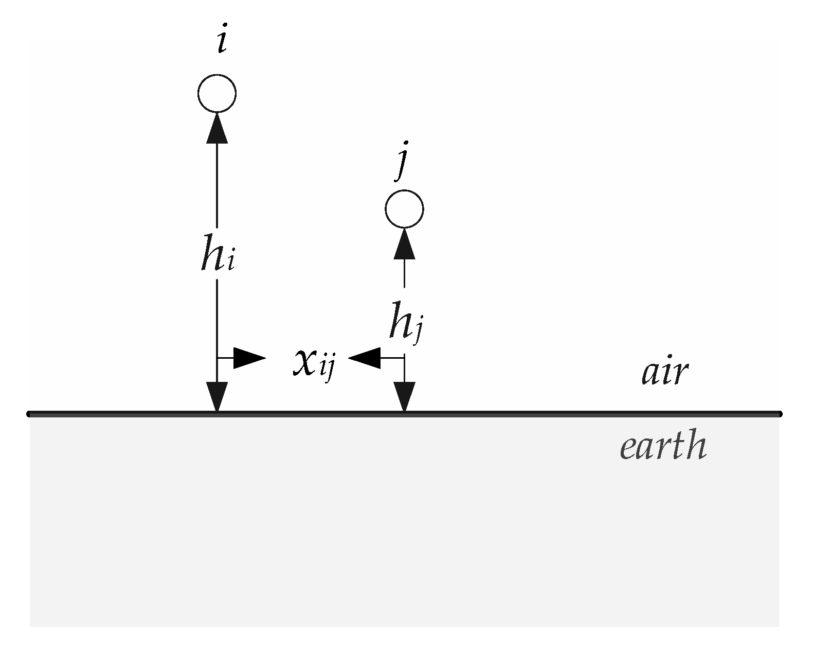
Figure 2.
Overhead line (OHL) configuration.

Figure 3.
Normalized sensitivities of the mutual impedance for (a) narrow-band (NB) and (b) broad-band (BB).
Figure 3.
Normalized sensitivities of the mutual impedance for (a) narrow-band (NB) and (b) broad-band (BB).

Figure 4.
Normalized sensitivities of the mutual admittance for (a) NB and (b) BB.
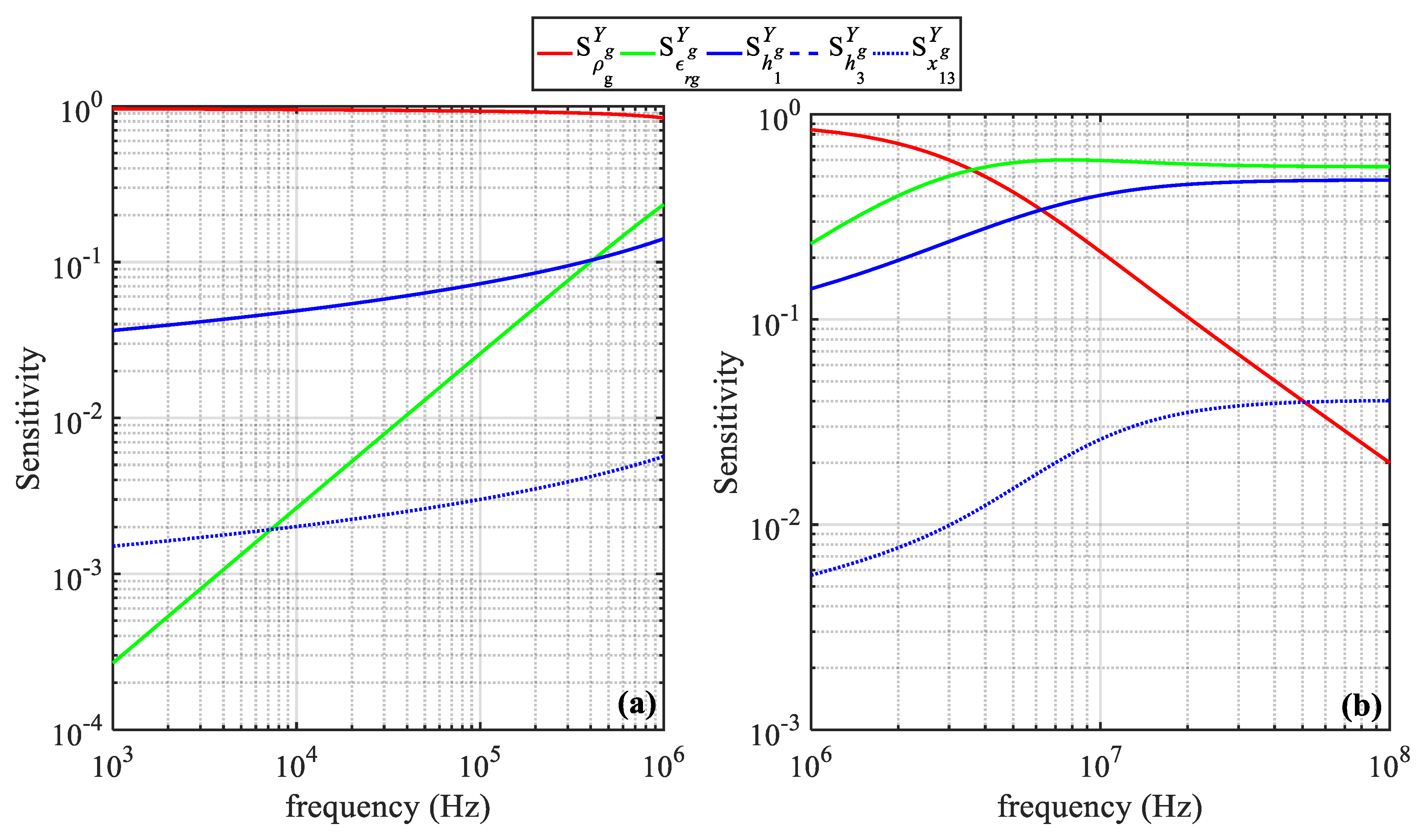
Figure 5.
Differences in Z11 in NB. For ρg = 100 Ωm, εrg = 1, (a) real part and (b) imaginary part, for ρg = 1000 Ωm, εrg = 1, (c) real part and (d) imaginary part.
Figure 5.
Differences in Z11 in NB. For ρg = 100 Ωm, εrg = 1, (a) real part and (b) imaginary part, for ρg = 1000 Ωm, εrg = 1, (c) real part and (d) imaginary part.

Figure 6.
Differences in Z11 in BB. For ρg = 100 Ωm, εrg = 1 and (a) real part, (b) imaginary part, for ρ1 = 1000 Ωm, εrg = 1 and (c) real part, (d) imaginary part.
Figure 6.
Differences in Z11 in BB. For ρg = 100 Ωm, εrg = 1 and (a) real part, (b) imaginary part, for ρ1 = 1000 Ωm, εrg = 1 and (c) real part, (d) imaginary part.

Figure 7.
Differences in Z13 in NB. For ρg = 100 Ωm, εrg = 1 and (a) real part, (b) imaginary part, for ρg = 1000 Ωm, εrg = 1 and (c) real part, (d) imaginary part.
Figure 7.
Differences in Z13 in NB. For ρg = 100 Ωm, εrg = 1 and (a) real part, (b) imaginary part, for ρg = 1000 Ωm, εrg = 1 and (c) real part, (d) imaginary part.
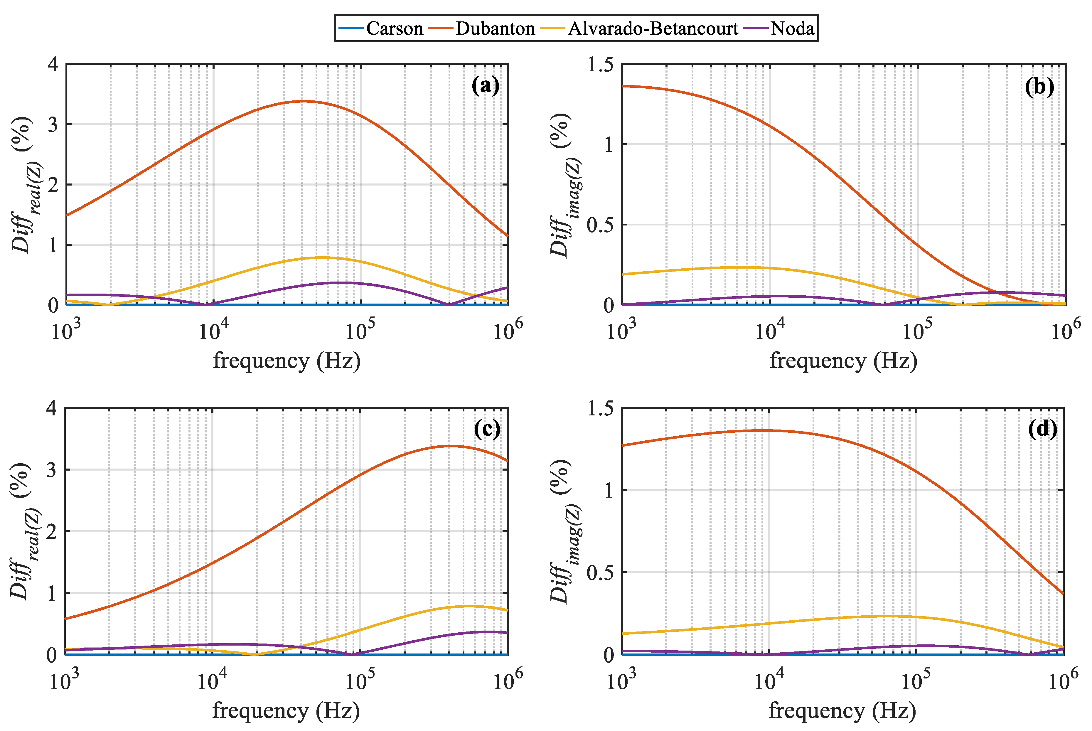
Figure 8.
Differences in Z13 in BB. For ρg = 100 Ωm, εrg = 1 and (a) real part, (b) imaginary part, for ρg = 1000 Ωm, εrg = 1 and (c) real part, (d) imaginary part.
Figure 8.
Differences in Z13 in BB. For ρg = 100 Ωm, εrg = 1 and (a) real part, (b) imaginary part, for ρg = 1000 Ωm, εrg = 1 and (c) real part, (d) imaginary part.

Figure 9.
Differences in the real part of Z13 in NB using the closed-form expression of (a) Carson, (b) Dubanton (c) Noda and (d) Alvarado-Betancourt.
Figure 9.
Differences in the real part of Z13 in NB using the closed-form expression of (a) Carson, (b) Dubanton (c) Noda and (d) Alvarado-Betancourt.

Figure 10.
Differences in the imaginary part of Z13 in NB using the closed-form expression of (a) Carson, (b) Dubanton (c) Noda and (d) Alvarado-Betancourt.
Figure 10.
Differences in the imaginary part of Z13 in NB using the closed-form expression of (a) Carson, (b) Dubanton (c) Noda and (d) Alvarado-Betancourt.
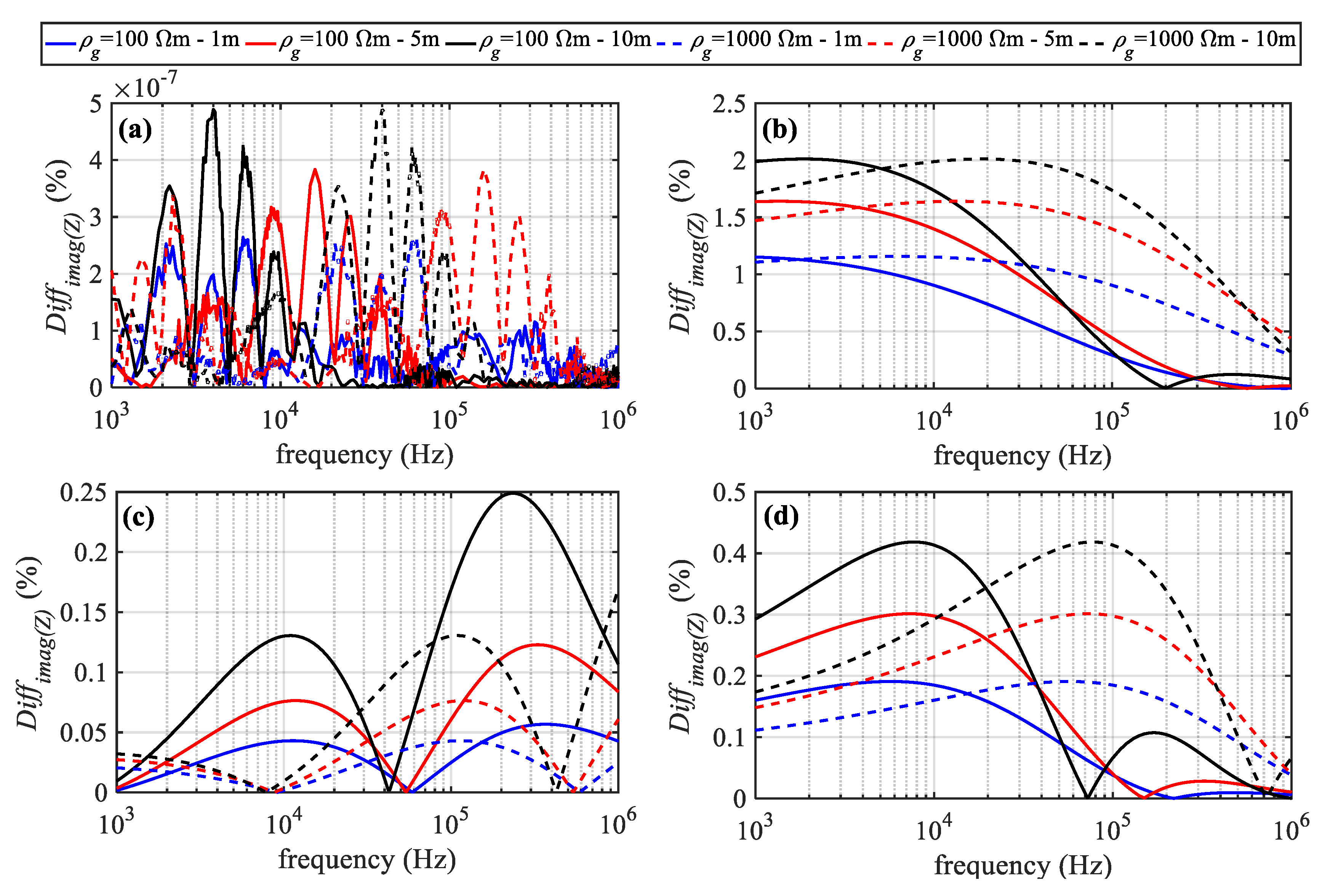
Figure 11.
Differences in the real part of Z13 in BB using the closed-form expression of (a) Carson, (b) Dubanton (c) Noda and (d) Alvarado-Betancourt.
Figure 11.
Differences in the real part of Z13 in BB using the closed-form expression of (a) Carson, (b) Dubanton (c) Noda and (d) Alvarado-Betancourt.

Figure 12.
Differences in the imaginary part of Z13 in BB using the closed-form expression of (a) Carson, (b) Dubanton (c) Noda and (d) Alvarado-Betancourt.
Figure 12.
Differences in the imaginary part of Z13 in BB using the closed-form expression of (a) Carson, (b) Dubanton (c) Noda and (d) Alvarado-Betancourt.
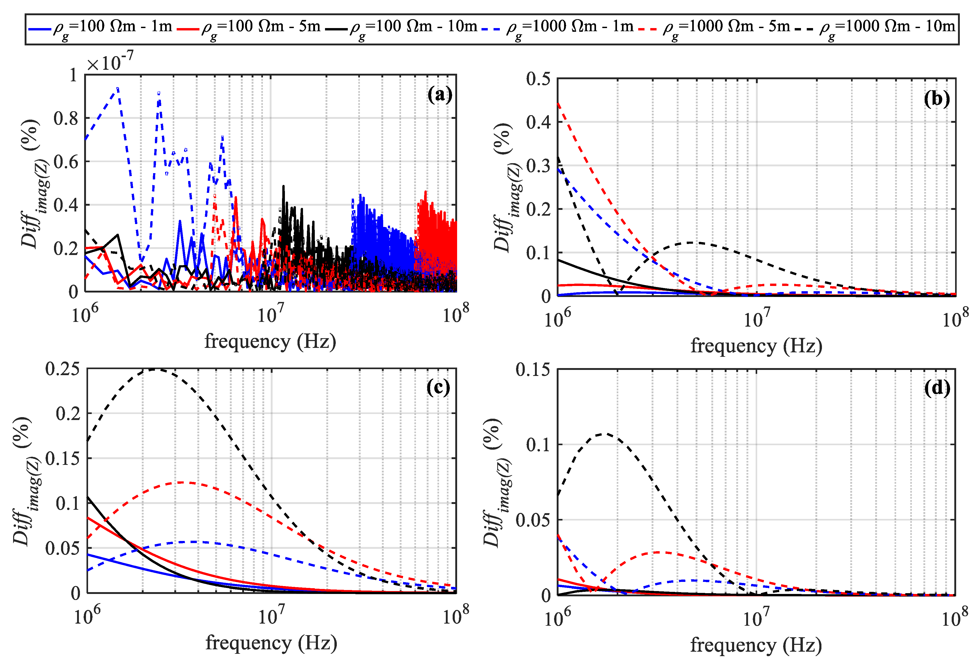
Figure 13.
Differences in the real part of Z13 in NB using the closed-form expression of (a) Carson, (b) Dubanton (c) Noda and (d) Alvarado-Betancourt.
Figure 13.
Differences in the real part of Z13 in NB using the closed-form expression of (a) Carson, (b) Dubanton (c) Noda and (d) Alvarado-Betancourt.

Figure 14.
Differences in the imaginary part of Z13 in NB using the closed-form expression of (a) Carson, (b) Dubanton (c) Noda and (d) Alvarado-Betancourt.
Figure 14.
Differences in the imaginary part of Z13 in NB using the closed-form expression of (a) Carson, (b) Dubanton (c) Noda and (d) Alvarado-Betancourt.

Figure 15.
Differences in the real part of Z13 in NB using the closed-form expression of (a) Carson, (b) Dubanton (c) Noda and (d) Alvarado-Betancourt.
Figure 15.
Differences in the real part of Z13 in NB using the closed-form expression of (a) Carson, (b) Dubanton (c) Noda and (d) Alvarado-Betancourt.
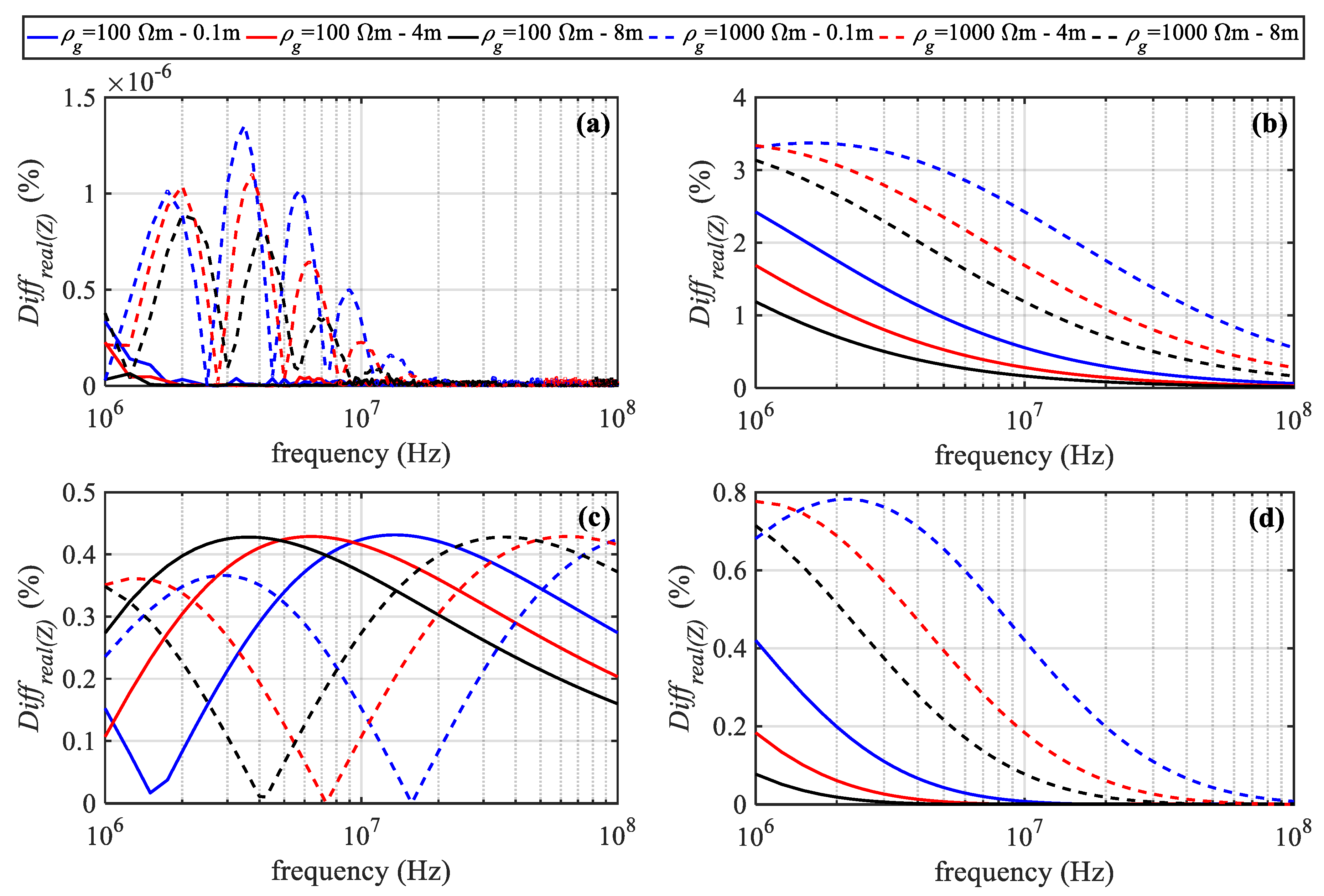
Figure 16.
Differences in the imaginary part of Z13 in NB using the closed-form expression of (a) Carson, (b) Dubanton (c) Noda and (d) Alvarado-Betancourt.
Figure 16.
Differences in the imaginary part of Z13 in NB using the closed-form expression of (a) Carson, (b) Dubanton (c) Noda and (d) Alvarado-Betancourt.
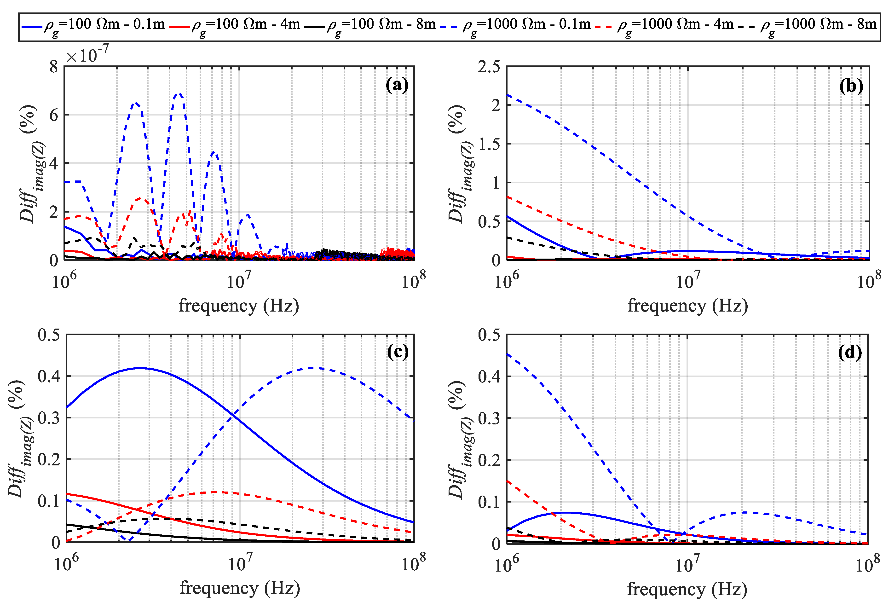
Figure 17.
Differences in Z13 in NB. For ρg = 100 Ωm, εrg = 10, (a) real part, (b) imaginary part, for ρg = 1000 Ωm, εrg = 10, (c) real part and (d) imaginary part.
Figure 17.
Differences in Z13 in NB. For ρg = 100 Ωm, εrg = 10, (a) real part, (b) imaginary part, for ρg = 1000 Ωm, εrg = 10, (c) real part and (d) imaginary part.

Figure 18.
Differences in Z13 in BB. For ρg = 100 Ωm, εrg = 10, (a) real part, (b) imaginary part, for ρg = 1000 Ωm, εrg = 10, (c) real part and (d) imaginary part.
Figure 18.
Differences in Z13 in BB. For ρg = 100 Ωm, εrg = 10, (a) real part, (b) imaginary part, for ρg = 1000 Ωm, εrg = 10, (c) real part and (d) imaginary part.
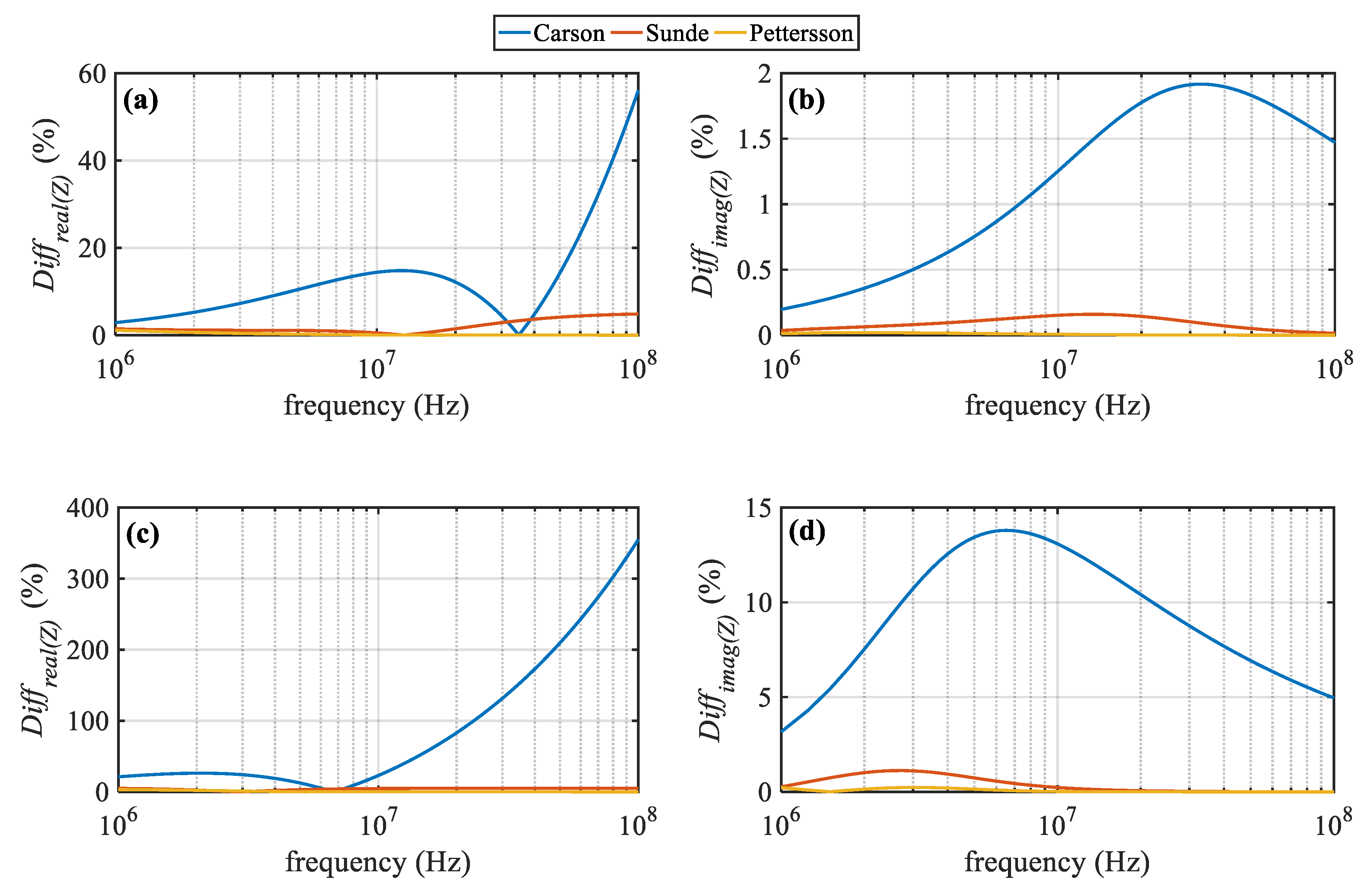
Figure 19.
Differences in Y13 at the NB frequency zone. For ρg = 100 Ωm, εrg = 10, (a) magnitude, (b) angle, for ρg = 1000 Ωm, εrg = 10, (c) magnitude and (d) angle.
Figure 19.
Differences in Y13 at the NB frequency zone. For ρg = 100 Ωm, εrg = 10, (a) magnitude, (b) angle, for ρg = 1000 Ωm, εrg = 10, (c) magnitude and (d) angle.

Figure 20.
Differences in Y13 at the BB frequency zone. For ρg = 100 Ωm, εrg = 10, (a) magnitude, (b) angle, for ρg = 1000 Ωm, εrg = 10, (c) magnitude and (d) angle.
Figure 20.
Differences in Y13 at the BB frequency zone. For ρg = 100 Ωm, εrg = 10, (a) magnitude, (b) angle, for ρg = 1000 Ωm, εrg = 10, (c) magnitude and (d) angle.
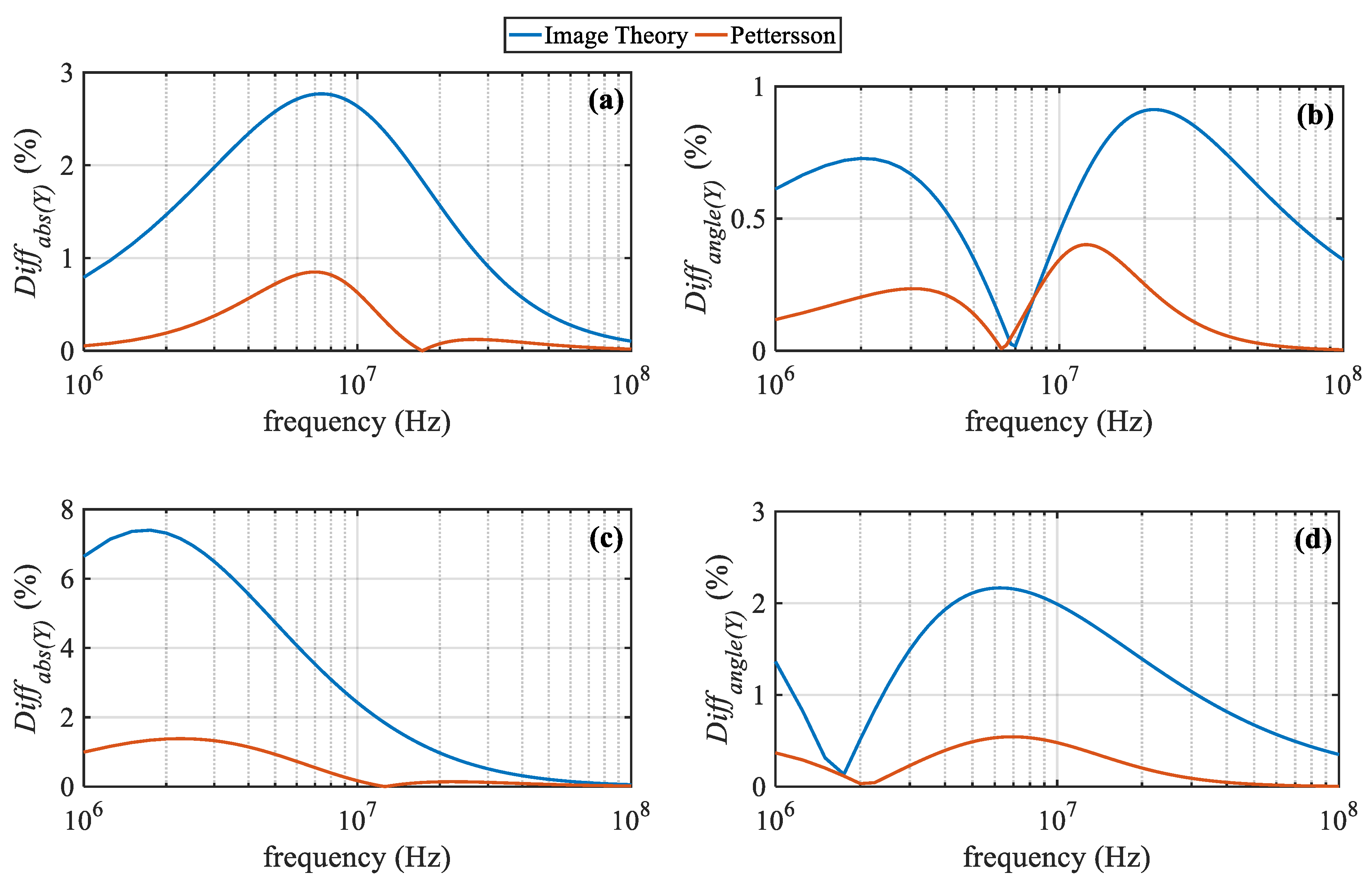
Figure 21.
Ground mode attenuation constant in (a) NB and (b) BB.

Figure 22.
Ground mode (a) attenuation constant, (b) characteristic impedance magnitude and magnitude of the (c) element (1,1) and (d) element (1,2) of the transformation matrix for different methods. NB range.
Figure 22.
Ground mode (a) attenuation constant, (b) characteristic impedance magnitude and magnitude of the (c) element (1,1) and (d) element (1,2) of the transformation matrix for different methods. NB range.

Figure 23.
Ground mode (a) attenuation constant, (b) characteristic impedance magnitude and magnitude of the (c) element (1,1) and (d) element (1,2) of the transformation matrix for different methods. BB range.
Figure 23.
Ground mode (a) attenuation constant, (b) characteristic impedance magnitude and magnitude of the (c) element (1,1) and (d) element (1,2) of the transformation matrix for different methods. BB range.
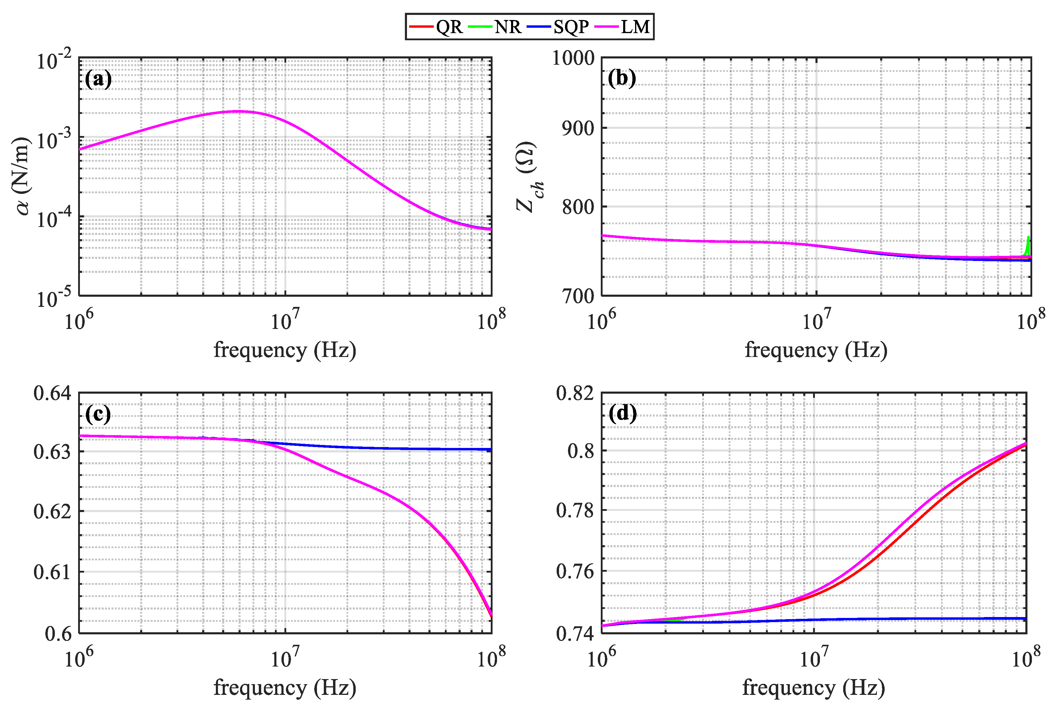
Figure 24.
Percentage difference in the injected signal level at the receiving end of conductor 1. Wire-to-ground (WTG) injection in (a) NB and (b) BB.
Figure 24.
Percentage difference in the injected signal level at the receiving end of conductor 1. Wire-to-ground (WTG) injection in (a) NB and (b) BB.

Figure 25.
Percentage difference in crosstalk at the receiving end of conductor 2. WTG injection in (a) NB and (b) BB.
Figure 25.
Percentage difference in crosstalk at the receiving end of conductor 2. WTG injection in (a) NB and (b) BB.

Figure 26.
Injected signal at the receiving end of phase a. Signal injection in (a) NB and (b) BB.

Figure 27.
Crosstalk at the receiving end of phase b. Signal injection in (a) NB and (b) BB.
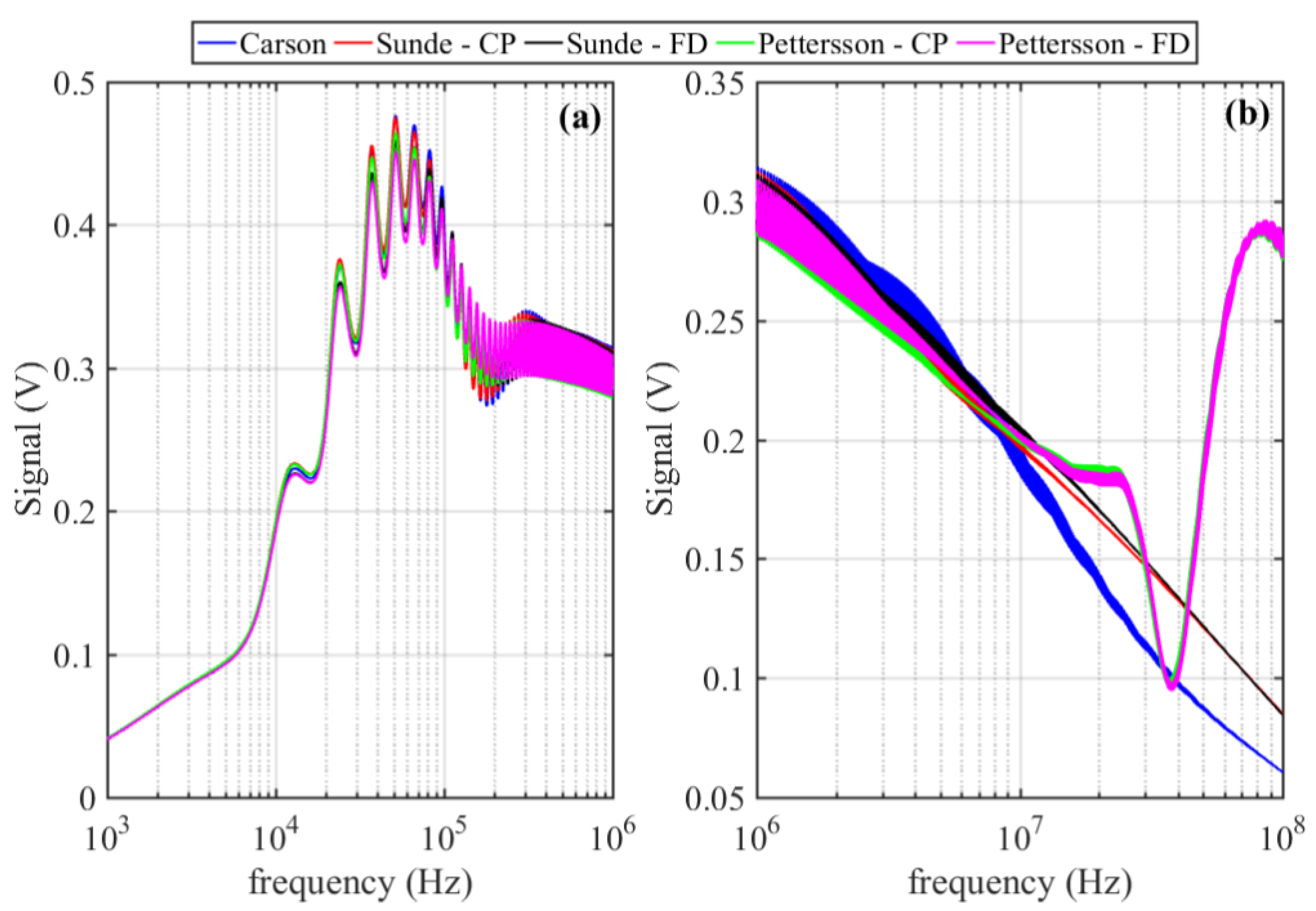
Figure 28.
Transient responses at the receiving end for ℓ = 0.5 km and (a) conductor 1, (b) conductor 2, for ℓ = 1.0 km and (c) conductor 1, (d) conductor 2, for ℓ = 10.0 km and (e) conductor 1, (f) conductor 2.
Figure 28.
Transient responses at the receiving end for ℓ = 0.5 km and (a) conductor 1, (b) conductor 2, for ℓ = 1.0 km and (c) conductor 1, (d) conductor 2, for ℓ = 10.0 km and (e) conductor 1, (f) conductor 2.

© 2020 by the authors. Licensee MDPI, Basel, Switzerland. This article is an open access article distributed under the terms and conditions of the Creative Commons Attribution (CC BY) license (http://creativecommons.org/licenses/by/4.0/).
Share and Cite
MDPI and ACS Style
Papadopoulos, T.A.; Chrysochos, A.I.; Traianos, C.K.; Papagiannis, G. Closed-Form Expressions for the Analysis of Wave Propagation in Overhead Distribution Lines. Energies 2020, 13, 4519. https://doi.org/10.3390/en13174519
AMA Style
Papadopoulos TA, Chrysochos AI, Traianos CK, Papagiannis G. Closed-Form Expressions for the Analysis of Wave Propagation in Overhead Distribution Lines. Energies. 2020; 13(17):4519. https://doi.org/10.3390/en13174519
Chicago/Turabian StylePapadopoulos, Theofilos A., Andreas I. Chrysochos, Christos K. Traianos, and Grigoris Papagiannis. 2020. "Closed-Form Expressions for the Analysis of Wave Propagation in Overhead Distribution Lines" Energies 13, no. 17: 4519. https://doi.org/10.3390/en13174519
Note that from the first issue of 2016, this journal uses article numbers instead of page numbers. See further details here.