Source Diagnosis of Solid Oxide Fuel Cell System Oscillation Based on Data Driven

1
College of Computer Science and Technology, Wuhan University of Science and Technology, Wuhan 430065, China
2
Hubei Province Key Laboratory of Intelligent Information Processing and Real-time Industrial System, Wuhan 430065, China
3
State Key Laboratory of Materials Processing and Die & Mould Technology, Huazhong University of Science and Technology, Wuhan 430074, China
4
School of Artificial Intelligence and Automation, Huazhong University of Science and Technology, Wuhan 430074, China
*
Author to whom correspondence should be addressed.
Energies 2020, 13(16), 4069; https://doi.org/10.3390/en13164069
Submission received: 27 April 2020
/
Revised: 8 July 2020
/
Accepted: 24 July 2020
/
Published: 6 August 2020
(This article belongs to the Special Issue Renewables-Based Microgrids)
Abstract
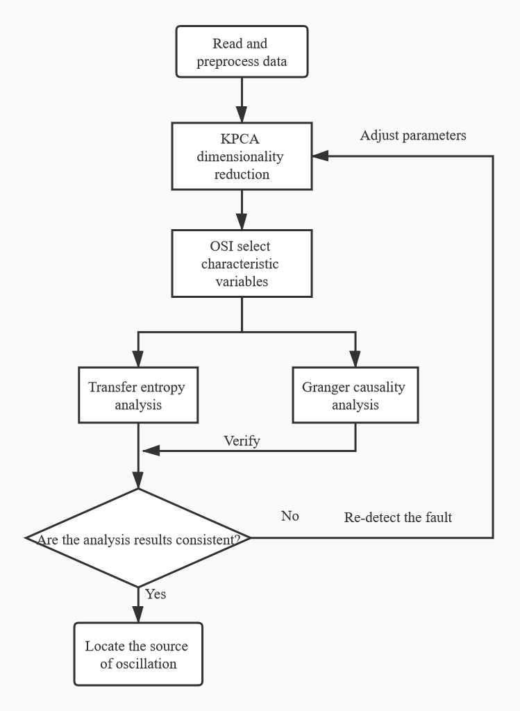
:The solid oxide fuel cell (SOFC) is a new energy technology that has the advantages of low emissions and high efficiency. However, oscillation and propagation often occur during the power generation of the system, which causes system performance degradation and reduced service life. To determine the root cause of multi-loop oscillation in an SOFC system, a data-driven diagnostic method is proposed in this paper. In our method, kernel principal component analysis (KPCA) and transfer entropy were applied to the system oscillation fault location. First, based on the KPCA method and the Oscillation Significance Index (OSI) of the system process variable, the process variables that were most affected by the oscillations were selected. Then, transfer entropy was used to quantitatively analyze the causal relationship between the oscillation variables and the oscillation propagation path, which determined the root cause of the oscillation. Finally, Granger causality (GC) analysis was used to verify the correctness of our method. The experimental results show that the proposed method can accurately and effectively locate the root cause of the SOFC system’s oscillation.

1. Introduction
The solid oxide fuel cell (SOFC) has the advantages of having low emissions and being noise-free and highly efficient in power generation. These cells have broad application prospects and have attracted widespread attention at home and abroad [1,2]. However, the development of China’s SOFC system is still in the developmental stage. The preliminary exploration of integration and control of an SOFC system has been completed in China, and a kW-class SOFC independent power generation system prototype has been successfully built. Due to the instability of temperature, pressure, flow, and other factors in the actual power generation process, the corresponding electrochemical reaction is affected, thereby reducing the SOFC system’s performance [3]. An SOFC system contains multiple subsystems and each of these contains multiple variables [4]. Therefore, when a certain part oscillates, it affects other parts and even the entire system, thus affecting the performance and life of the entire system [5]. In order to reduce the performance degradation caused by the SOFC system’s oscillation and extend the SOFC’s service life, it is particularly important to diagnose the root cause of the SOFC system’s oscillation.
In the existing literature, much research has been carried out on the fault diagnosis of an SOFC system. Vijay et al. [6] proposed a nonlinear observer-based fault diagnosis strategy. Two nonlinear adaptive observers were designed to uniquely identify and diagnose all common faults in the SOFC. Costamagna et al. [7] adapted the supervised classifier to the new conditions through domain adaptive statistics technology, solved the fault diagnosis under unexpected non-design operating conditions, and reduced the decrease in diagnostic performance. Wu et al. [8] proposed a statistical method based on principal component analysis (PCA) and an exponentially weighted moving average control chart for SOFC system gas supply fault detection. Wu et al. [9] developed a predictive controller to solve the thermal power surge problem and improved the energy conversion efficiency of the SOFC system. Xu et al. [10] developed an adaptive energy management algorithm to ensure the thermal safety of the SOFC system. Xue et al. [11] used a Bayesian regularized neural network for fault diagnosis and designed a fuzzy fault-tolerant control strategy for thermal safety problems of the SOFC system.
There are also many studies on online monitoring tools for SOFC systems. Fan et al. [12] designed a dissolved gas analysis (DGA) online monitor based on an SOFC gas sensor, which can accurately measure the gas in the power transformer and detect early failures. Subotic et al. [13] designed a tool for online monitoring of the critical frequency of carbon deposition in the SOFC system, which is of great significance for isolating the critical feedback frequency in practical experiments. Dolenc et al. [14] used variational estimation of the nonlinear coupling function Bayesian inference to monitor SOFC system performance. Wu et al. [15] built the Elman neural network state prediction model under the entire stage experiment to predict the future voltage and the health state of the SOFC system.
According to the literature survey, there is much literature addressing the oscillation diagnosis of an SOFC system. The methods for identifying root causes of plant-wide oscillations are mainly divided into two categories, namely model-based and data-based methods [5]. The model-based method requires a deep understanding of the system workflow and process characteristics and can accurately describe the system process knowledge to obtain the system oscillation propagation path. Yim et al. [16] used the process schematic of a plant control loop performance assessment. Jiang et al. [17] proposed the concept of adjacency matrix and reachability matrix to find the root cause of plant-wide oscillations. Yang et al. [18] used the signed directed graph (SDG) model to describe the causality between variables and analyzed the propagation of faults in industrial systems. However, the model-based method has the disadvantages of difficult information extraction and model description [5]. Data-based methods are widely used in oscillation diagnosis. The data-driven causal analysis method is a time series analysis method. It uses historical process data to measure the degree of interaction between process variables and then obtains the causal relationship between the variables. Unlike model-based methods, data-driven analysis methods do not require prior knowledge of the system’s internal information and can quantitatively estimate the level of interaction between variables. Therefore, data-based methods are widely used to deal with oscillation diagnosis problems. The data-driven approaches do not require complex prior information knowledge within the system, and the data are relatively easy to obtain through experimentation. Thornhill et al. [19] proposed a nonlinearity index of process variables for oscillation diagnosis. Xia and Howell [20] proposed a nonlinearity method that included a variance index to indicate possible root cause. Xia et al. [21] used multi-resolution spectral independent component analysis and a significance index to detect the source of multiple oscillations. Jiang et al. [22] proposed an oscillation contribution index (OCI) to evaluate the contribution of each variable to plant-wide oscillation and isolate the key variables as the potential root cause. The Granger causality (GC) was used for root cause diagnosis of plant-wide oscillations in reference [23]. The proposed method applies both time-domain Granger causality and spectral Granger causality to provide a new diagnostic guidance. Zhong et al. [24] combined Granger causality analysis with adjacency matrix to diagnose the root cause of SOFC system oscillation. Xu et al. [25] combined spectral envelope and transfer entropy to provide a reliable diagnosis of oscillation sources and propagations. It turns out that the Granger causality is easier to implement and the computational cost in reference [26] is much less, but it only applies to linear relationships between variables, and model misidentification may occur. Transfer entropy applies to linear and nonlinear relationships between variables and can give more accurate results than the Granger causality [26]. Transfer entropy has been successfully applied to oscillation diagnosis in chemical processes [27].
In this paper, a 1kW steam reforming SOFC system was studied. In order to ensure the good performance of an SOFC system, transfer entropy was used to diagnose the root cause of system oscillation, which combines data-driven and expert experience. The purpose of this article was to diagnose the root cause of oscillations of an SOFC system. Since some variables in the system were not related to oscillation problems, they could be eliminated during the research process. Because of the large computation complexity of transfer entropy, it was necessary to select the characteristic variables first. The characteristic variables were good for the interpretability and understanding of the oscillation root causes. Therefore, the selection of characteristic variables is important in analyzing and diagnosing the root cause of an SOFC system’s oscillation. PCA is a common data dimensionality reduction method, but it is only applicable to linear data that obey Gaussian distribution. The nonlinear correlation between samples may be lost after linear dimensionality reduction using PCA. Therefore, a method combining kernel principal component analysis (KPCA) and the Oscillation Significance Index (OSI) was first proposed to select characteristic variables [23]. Then, transfer entropy was used to quantitatively analyze the causal relationship between the oscillation variables, which combines the system connectivity rules, to determine the root cause of the system oscillation. Finally, the Granger causality analysis method was used to verify the effectiveness of our method.
2. Description of the SOFC System
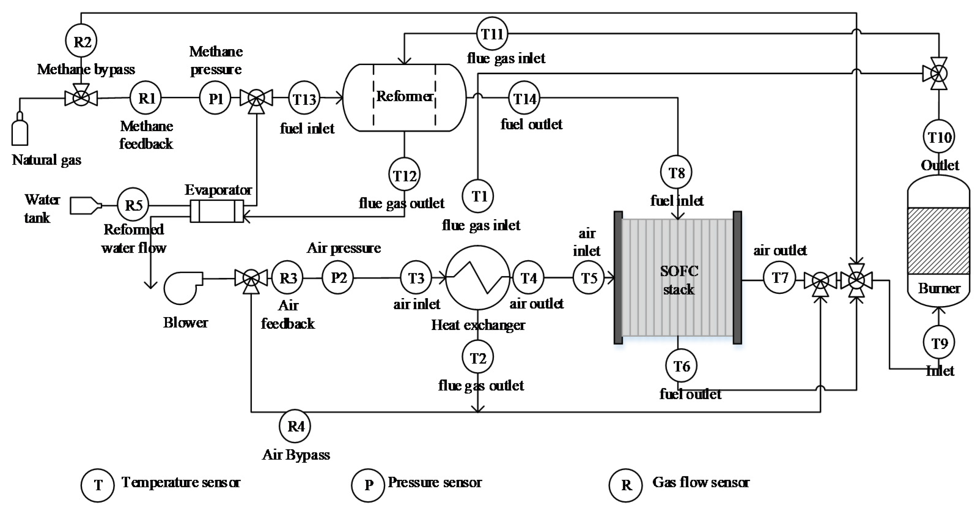
The schematic diagram of the 1 kW SOFC system for the experiment is shown in Figure 1. The system consists of an SOFC stack, a reformer subsystem, a heat exchanger subsystem, a fuel supply subsystem, an air supply subsystem, a water tank, a combustion chamber, a power converter, and a control system. The distribution of the main sensors is also given. These sensors measure the data of a total of 24 process variables, including gas flow, pressure, and internal temperature of each component. The SOFC system uses methane as fuel, and water is provided by a water tank. The reforming reaction between fuel and deionized water in the reformer generates hydrogen and carbon monoxide. This process requires a certain amount of water and heat. On the air side, a blower provides enough air to the system, and the air is heated by the heat exchanger to the required inlet set temperature. Once the fuel and air flow reach the SOFC stack, an electrochemical reaction occurs, generating the required electrical energy. For the power to reach the end user, a power converter is required to convert DC power to AC power. The leak of the stack gas burns in the combustion chamber and reduces pollutant emissions. The heated gas reaches the reformer, which can control the reforming reaction temperature. It then flows through the heat exchanger to heat the fresh air provided by the blower. In addition, the system also has an automatic protection shutdown function, including the upper and lower limits of temperature, flow, and pressure, and automatically enters the protective gas after shutdown.
There are many monitoring variables throughout the power generation process, including 24 process variables, some of which are described in Table 1.
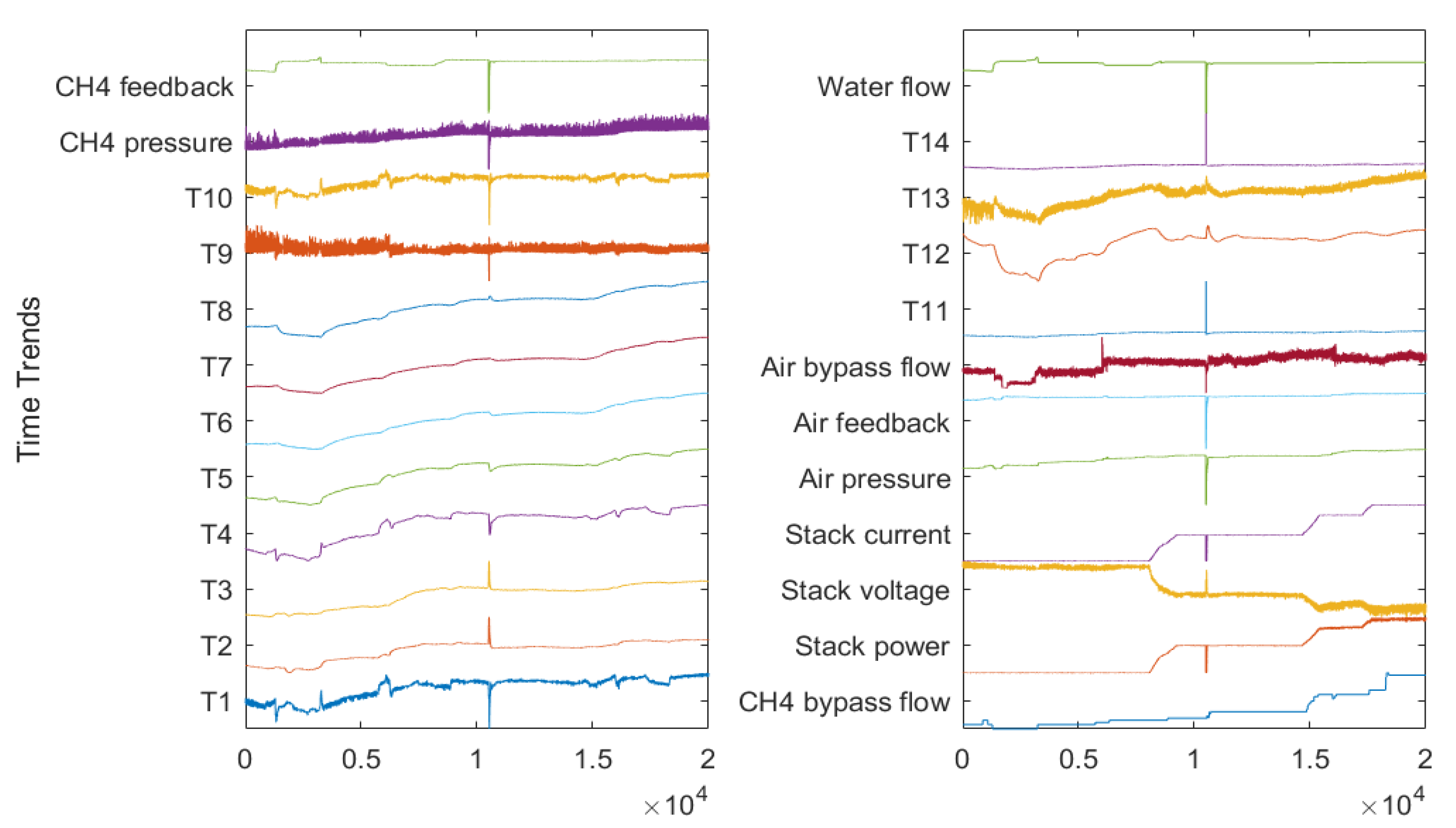
In order to evaluate the performance of the SOFC system and find the root cause of the system oscillation, it was necessary to obtain data for each variable of the SOFC system under the entire operating conditions. The experimental phase included start, stop, standby, and long-term discharge phases. The 1 kW SOFC system with steam reforming included 36 measurement variables in the entire power generation process, and 24 variables were selected to form the main control loop of the SOFC system, including gas flow, pressure, and internal temperature measurement data for each component, as well as electrical characteristic data. We collected data for the 24 process variables from the system every 1 second for oscillation fault analysis. Figure 2 shows the normalized time trend curve of 20,000 sample data for 24 process variables. It can be seen from the figure that nearly half of the process variables had different degrees of oscillation. Due to the large number of variables involved in the entire power generation process and the complex correlation of the control loop, the oscillation signal can be easily propagated in multiple control loops, so it is difficult to directly determine the root cause of the oscillation in the SOFC system.
3. Diagnosis Method for the SOFC System’s Oscillation
3.1. Characteristic Variable Selection
Many of the process variables in the SOFC system’s oscillation process have nothing to do with the oscillation problem. In order to improve the accuracy of the oscillation diagnosis and reduce the amount of transfer entropy calculation, it was necessary to first reduce the data dimension and filter the characteristic variables. PCA is the most common data dimensionality reduction algorithm, but it can only deal with the dimensionality reduction of linear data that obey Gaussian distribution. It often has a poor effect on linearly inseparable data. Therefore, in order to eliminate the nonlinear correlation between data and reduce the data dimension, the KPCA method was used. The key of the KPCA method is to use a nonlinear mapping function to map the related data set to the high-dimensional feature space. This is followed by the traditional PCA carried out to select significant oscillation variables from the original process data [28,29].
Here we assume that the sample data are and means the number of samples, is the dimension of the samples, is a nonlinear transformation, is a mapping space, and the image of the original data in space is . When , the covariance matrix of the mapping data is defined as follows:
The Eigen decomposition of the covariance matrix is as follows:
where is the eigenvalue of the covariance matrix, and is the eigenvector corresponding to the covariance matrix. The kernel function is defined by the following:
In the equation, is a kernel function matrix generated by the kernel function. There are many commonly used kernel functions. The kernel function used in this paper is the Gaussian radial basis kernel function; σ is the width parameter of the function and controls the radial action range of the function.
The obtained eigenvalues are arranged in descending order, and the corresponding eigenvector units are orthogonalized. The first components are extracted based on the principal component contribution rate, and finally the projection of the kernel matrix on a partial eigenvector is obtained. The cumulative variance contribution rate is the ratio of the sum of the main t-dimensional principal component variance contribution rates to the total n-dimensional principal component variance contribution rate, and the ratio is directly proportional to the information containing metadata. Generally, when the cumulative variance contribution ratio of the principal components of the first t dimensions of exceeds 85%, the original n-dimensional data information can be characterized by the t-dimensional data information to achieve the purpose of reducing dimensions [30] as follows:
where is a measure of the contribution of the original variable to the principal component . According to the Oscillation Significance Index (OSI), process variables that have a significant contribution to the principal component are selected to construct a subset of oscillation failure analysis as follows:
In the equation, is a eigenvalue corresponding to the principal component in the oscillation source candidate variable set .
3.2. Transfer Entropy
Transfer entropy is an information theoretical explanation of the causal relationship between two variables. For two different time series X and Y, assuming that is influenced by the former k states of the sequence X and the former l states of the sequence Y, the transfer entropy from Y to X can be calculated using the following equation, which represents a reduction in the uncertainty of Y when X is known [31]:
In actual situations, k = 1 and l = 1 are the better choices for calculation, which can avoid the evaluation of complex high-dimensional probability density functions when calculating transfer entropy. This does not affect the use of transfer entropy to determine the directionality and correlation between variables [32]; therefore, Equation (7) can be simplified as follows:
The reverse transfer entropy is as follows:
Finally, the causality measure can be calculated by subtracting the effect of X on Y from the effect of Y on X, as Equation (10):
means that Y causes X and means that X causes Y. When there are multiple variables, the results can be denoted in a causality matrix as follows:
The rows represent cause variables, while the columns represent the effect variables, and R represents the number of variables [27].
3.3. Granger Causality
The Granger causality (GC) test is a statistical method for hypothesis testing, which is used to test whether one set of time series has a causal effect on another set of time series . The basic principle is to establish an autoregressive model; under the condition of controlling the past value of , the prediction accuracy of the past value of to the current value of is estimated [33]. The GC method needs to input multivariate time series data to meet the requirements of generalized stationary, otherwise incorrect regression problems may occur. In order to ensure that the oscillation factor is the main information of the original data, and at the same time meet the generalized stationary requirements of vector autoregressive (VAR) modeling, it is necessary to perform smooth preprocessing on the original data such as a differential transformation operation to eliminate the time series trend. Granger causality testing is divided into time domain Granger causality analysis and frequency domain Granger causality analysis. Time domain Granger causality analysis is used to test the effectiveness of the proposed method.
The system operation historical data are composed of time series data of multiple process variables. The time series and of any two process variables are taken, and all the lag terms ,, of , and are regressed to establish a complete autoregressive (AR) model for predicting and :
In the equation, , , , and are the model coefficients, and are the model prediction errors, and is the model order that defines the number of lag terms included in the model.
Corresponding to the above complete model definition, the lag term of the variable is excluded and then regression is performed to establish a restricted model for predicting :
In the equation, refers to the model prediction error obtained without considering the prediction of to .
If the model prediction variance is significantly smaller than , its statistical significance is to combine the past value of and the prediction of is more accurate, which means produces a Granger causality for . Therefore, the Granger causality can be quantified by the following index:
Before performing Granger causality inference, the F-test was used to verify its statistical significance. If the F value calculated at the selected significance level (value set to 0.05) exceeds the critical value , it is satisfied that the p value is less than , indicating that is the cause of :
where m is the observation sample size; and are the sum of the residual squares of the restricted model and the complete model, respectively; is equal to the number of lag terms, that is, the number of parameters to be estimated in the restricted model; and is the number of parameters to be estimated in the complete model, which satisfies .
4. Results and Discussion
4.1. Characteristic Variable Selection
Before locating the oscillation faults of the SOFC system, the process variables affected by the oscillating signals were first screened from the original process data to reduce the scope of causal analysis and improve the accuracy of the oscillating source identification.
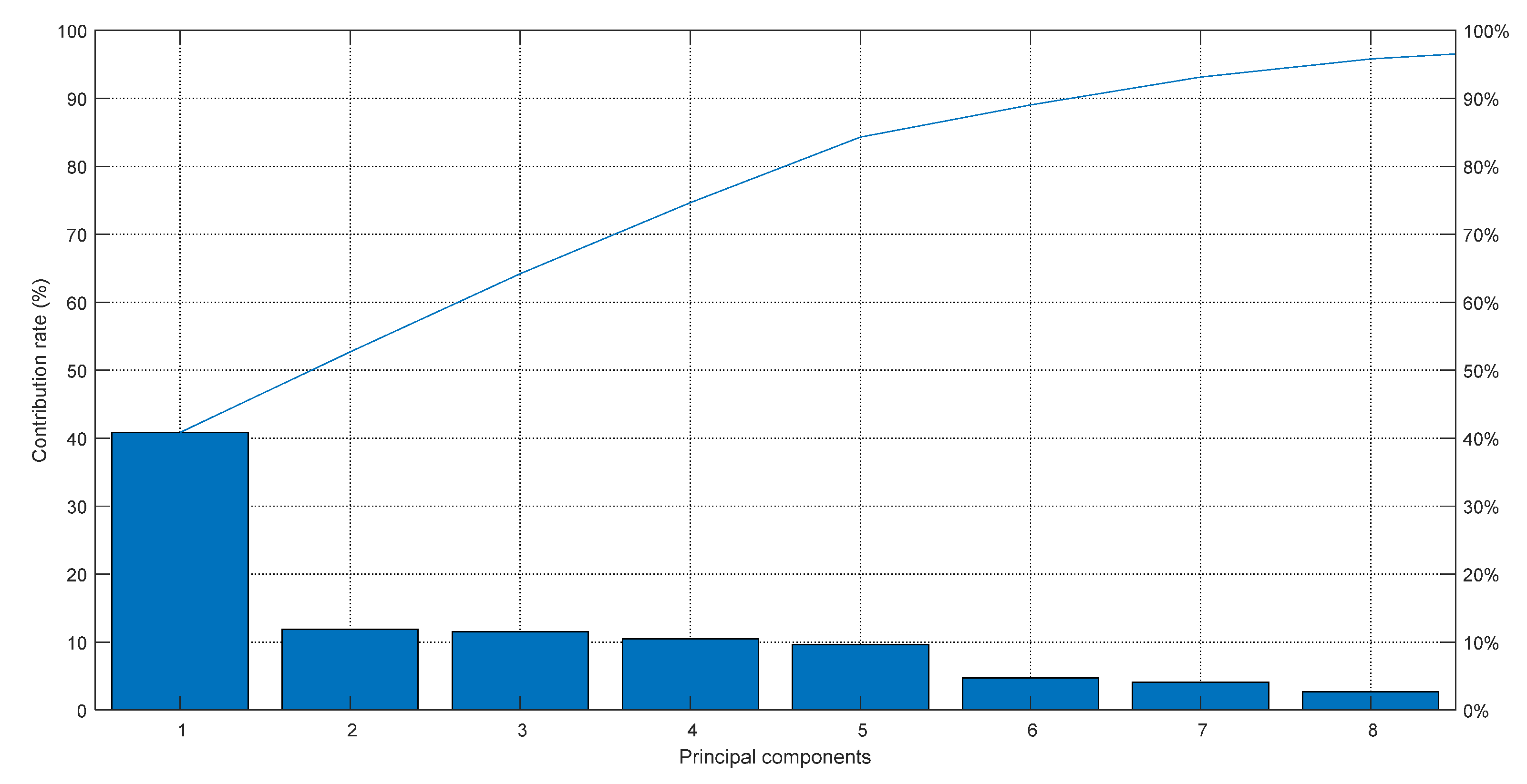
For this study, we normalized the original data and used KPCA to reduce the dimensionality of the normalized data. The result is shown in Figure 3. The 24 process variables are reduced to eight-dimensional principal components, and the sum of their contribution rates reaches more than 95%. In other words, the first eight principal components can reflect almost all the characteristics of the original data.
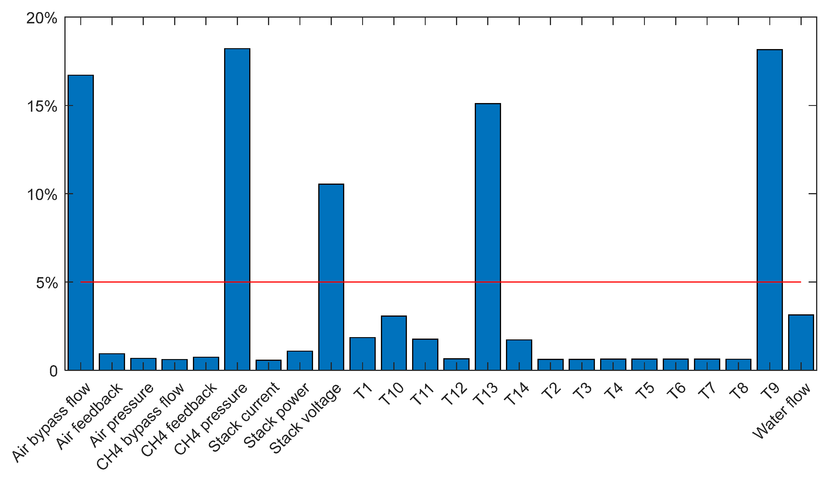
The OSI is calculated in the range of eight principal components, and variables with significant oscillations are screened out of all process variables on the condition that the percentage of OSI accounted for more than 5%. Figure 4 shows the result. The selected oscillating variables include combustion chamber inlet temperature, methane pressure, stack voltage, air bypass flow, and reformer fuel inlet temperature. It can be seen in Figure 2 that the filtering results of the oscillation variables are the five variables that are most affected by the oscillation among all process variables.
4.2. SOFC System Oscillation Diagnosis Results and Discussion
There are a large number of variables in the SOFC system, and the KPCA method was used to screen five characteristic variables with significant oscillations among the 24 original process variables. Subsequently, the method of transfer entropy was used for further research. The causality matrix of the transfer entropy analysis is shown in Table 2. An arbitrary position in the causality matrix represents the causality measure from the row variable to the column variable. It can be known from Equation (8) that the transfer entropy value from to and the transfer entropy value from to are opposite numbers to each other. The causal matrix is symmetrical about the diagonal. For example, the position (2,3) indicates that the transfer entropy value of methane pressure to the stack voltage is 0.4390, which is the largest of all causal measures. It indicates that the methane pressure has the largest impact on the stack voltage oscillation. The transfer entropy value of methane pressure to the inlet temperature of the combustion chamber is 0.2748, which also shows a significant causal effect. At the same time, we can clearly see that the transfer entropy values in the second row are all positive, and the transfer entropy values in the second column are all negative, which means that the methane pressure has an impact on other oscillatory variables and there is no other variable that affects methane. This shows that methane pressure is the root cause of the system oscillation.
As can be seen from the table, causal feedback exists in the remaining oscillation variables, reflecting the strong coupling characteristics of the system. However, it is important that the causal measures between the air bypass flow and other variables are very small. Based on the process knowledge, a reasonable explanation can be made as follows: the purpose of adding cold air bypass on the air trunk road is to pass excessive. The cold air effectively controls the temperature of the air at the inlet of the stack, thereby ensuring that the stack is in a thermally safe state. Compared with excess air feedback supply, fuel supply is the key to causing abnormal fluctuations in stack discharge. In addition, as can be seen in Figure 4, just like the air bypass flow, the air feedback flow and air pressure are also affected by the oscillation. However, due to the lower effect, it is filtered out in the filtering process of the oscillation variable. It can be concluded that the air volume fluctuation caused by the blower failure has no obvious relationship with the methane pressure.
In addition, it can be seen that the transfer entropy value of the burner chamber inlet temperature to the stack voltage is 0.0998. Combined with the structure flow chart of the SOFC system, a reasonable explanation can be made. The temperature of the burner chamber affects the temperature of the entire system and the stack. The temperature increase of the burner chamber will indirectly raise the temperature of the stack. In the case of constant current, the higher the temperature, the higher the voltage. Conversely, the lower the temperature, the lower the voltage [34].
According to the analysis of the transfer relationship between the variables in Table 2, it can be concluded that the methane pressure instability is the root cause of the oscillation fault, which directly affects the temperature fluctuation of the fuel inlet of the reformer, and then causes the voltage fluctuation of the stack, and finally causes the temperature fluctuation of the burner chamber inlet.
Combining the structure diagram of the system in Figure 1 and the results of the transfer entropy analysis, it can be concluded that the methane pressure is the source of oscillation in the SOFC system. As the fuel required for the operation of the SOFC system, methane flows along the pipeline to the reforming chamber to participate in the reforming reaction, participate in the electrochemical reaction in the anode runner of the stack, and participate in the oxidation reaction in the exhaust gas. Therefore, the supply of methane plays a vital role in the heat, electricity, and gas stability of the system. The methane feedback flow does not oscillate significantly, which can eliminate the cause of the instability of the flow velocity at the fuel supply end. According to the system structure diagram and the connectivity rules of each component, it can be concluded that the reason for methane pressure fluctuation is the deionized water vapor fluctuation in the reforming reaction.
4.3. Granger Causality Verification
The causal matrix based on time domain GC analysis is shown in Table 3. Any position in the causal matrix represents the causal metric from the column variable to the row variable. For example, the position (3,2) indicates that the Granger causality measure of methane pressure on the stack voltage is 0.4458, which is the largest of all causality measures, indicating that the methane pressure has the largest impact on the voltage of the stack. Table 4 shows the F-test result P value of each group of causality. When the P value is less than the significance level α (α = 0.05), the F-test result is valid and the causal inference is established. It is marked in bold in Table 4 and the corresponding causality measure is shown in bold in Table 3. It can be seen from Table 3 that the measurement of methane pressure on the inlet temperature of the burner chamber and the stack voltage shows a clear causal relationship. At the same time, it can be found that the methane pressure has the greatest influence on the chimney voltage, which is much higher than the causal value of the stack voltage change caused by other reasons. Therefore, it can be determined that methane pressure instability is the root cause of the oscillation fault.
Similarly, we can see that the causal relationship between air bypass flow and other variables is small. The F-test results show that the corresponding causal hypothesis is invalid, and the result is the same as that of the transfer entropy.
Combining the results of the two data analysis methods of transfer entropy and Granger causality analysis, it can be derived that the methane pressure is the source of the oscillation failure.
Since there is communication between the reforming reaction water vapor and the methane supply pipeline, the fluctuation of the water vapor affects the pressure fluctuation in the chamber, and further affects the pressure fluctuation of the methane. The fluctuation of water vapor in the evaporator cannot be monitored by the existing sensors. However, the set value of deionized water can be adjusted. Based on the results, we artificially reduced the set value of deionized water in the later stages of the experiment. As a result, the number of experimental shutdowns and fluctuations in methane pressure was greatly reduced. Therefore, the source of the oscillating failure is unstable methane pressure, which is the result closest to the root cause of the actual failure. Therefore, we can isolate or reduce the effect of water vapor on methane pressure, which can help the SOFC system achieve good performance and maintain its stability and long-term operation.
5. Conclusions
Based on the research of a 1 kW SOFC independent power generation system with steam reforming, a data-driven SOFC system root cause diagnosis method is proposed for the oscillation fault problem in the system. KPCA and transfer entropy were employed to locate the root cause of system oscillations. First, variables unrelated to the oscillation of the SOFC system were eliminated, then five characteristic variables were selected from the 24 original process variables based on KPCA and OSI. Subsequently, transfer entropy theory was used to calculate the direct causality of the variables and analyze the oscillation propagation path in combination with the system structure to successfully determine the source of the oscillation as methane pressure. Finally, the time domain Granger causality analysis method was used to prove the effectiveness and reliability of our method. The experimental results show that our method can diagnose the root cause of vibration based on the process data. The fault location effect is obvious, and the results are accurate and reliable. In addition, combining data analysis and expert experience, the proposed method can provide an effective method for diagnosing the root cause of oscillations in an SOFC system.
Author Contributions
Conceptualization and methodology, X.F. and Y.L.; writing, Y.L., X.F., and X.L.; supervision, project administration, and funding acquisition, X.F. and X.L. All authors have read and agreed to the published version of the manuscript.
Funding
This work was supported by the National Natural Science Foundation of China (No. 61873323), the Open Fund Project of the State Key Laboratory of Material Processing and Die & Mould Technology, Huazhong University of Science and Technology (No. P2018-016), the Hubei Provincial Natural Science Foundation of China (Nos. 2017CFB506 and 2016CFA037), the Wuhan Science and Technology Plan Project (No. 2018010401011292), the WUST National Defence Pre-Research Foundation (No. GF201912), and the Open Fund Project of the Hubei Province Key Laboratory of Intelligent Information Processing and Real-time Industrial System (Nos. 2016znss02A and znxx2018ZD01).
Acknowledgments
Thanks to Pu Jian from the Fuel Cell Research Center of Huazhong University of Science and Technology. Thanks to the Fuel Cell Research Center of Huazhong University of Science and Technology for providing experimental data.
Conflicts of Interest
The authors declare no conflict of interest.
References
- Bozorgmehri, S.; Hamedi, M. Modeling and Optimization of Anode-Supported Solid Oxide Fuel Cells on Cell Parameters via Artificial Neural Network and Genetic Algorithm. Fuel Cells 2012, 12, 11–23. [Google Scholar] [CrossRef]
- Wu, X.; Ye, Q. Fault diagnosis and prognostic of solid oxide fuel cells. J. Power Sources 2016, 321, 47–56. [Google Scholar] [CrossRef]
- Cao, H.; Li, X. Thermal Management-Oriented Multivariable Robust Control of a kW-Scale Solid Oxide Fuel Cell Stand-Alone System. IEEE Trans. Energy Convers. 2016, 31, 603–612. [Google Scholar] [CrossRef]
- Zhang, L.; Liu, J.; Qi, W.; Chen, Q.; Long, R.; Quan, S. A parallel modular computing approach to real-time simulation of multiple fuel cells hybrid power system. Int. J. Energy Res. 2019, 43, 5266–5283. [Google Scholar] [CrossRef]
- Duan, P.; Chen, T.; Shah, S.L.; Yang, F. Methods for root cause diagnosis of plant-wide oscillations. AIChE J. 2014, 60, 2019–2034. [Google Scholar] [CrossRef]
- Vijay, P.; Tade, M.O.; Shao, Z. Adaptive observer based approach for the fault diagnosis in solid oxide fuel cells. J. Process Control 2019, 84, 101–114. [Google Scholar] [CrossRef]
- Costamagna, P.; De Giorgi, A.; Moser, G.; Pellaco, L.; Trucco, A. Data-driven fault diagnosis in SOFC-based power plants under off-design operating conditions. Int. J. Hydrog. Energy 2019, 44, 29002–29006. [Google Scholar] [CrossRef]
- Wu, X.L.; Xu, Y.W.; Zhao, D.Q.; Li, Z.H.; Zhong, X.B.; Chen, M.T.; Jiang, J.H.; Deng, Z.H.; Fu, X.W.; Li, X. Fault detection and assessment for solid oxide fuel cell system gas supply unit based on novel principal component analysis. J. Power Sources 2019, 436, 226864. [Google Scholar] [CrossRef]
- Wu, X.-l.; Xu, Y.-w.; Zhao, D.-q.; Zhong, X.-b.; Li, D.; Jiang, J.; Deng, Z.; Fu, X.; Li, X. Extended-range electric vehicle-oriented thermoelectric surge control of a solid oxide fuel cell system. Appl. Energy 2020, 263, 114628. [Google Scholar] [CrossRef]
- Xu, Y.-w.; Wu, X.-l.; Zhong, X.; Zhao, D.; Fu, J.; Jiang, J.; Deng, Z.; Fu, X.; Li, X. Development of solid oxide fuel cell and battery hybrid power generation system. Int. J. Hydrog. Energy 2020, 45, 8899–8914. [Google Scholar] [CrossRef]
- Xue, T.; Wu, X.; Zhao, D.; Xu, Y.; Jiang, J.; Deng, Z.; Fu, X.; Li, X. Fault-tolerant control for steam fluctuation in SOFC system with reforming units. Int. J. Hydrog. Energy 2019, 44, 23360–23376. [Google Scholar] [CrossRef]
- Fan, J.; Fu, C.; Yin, H.; Wang, Y.; Jiang, Q. Power transformer condition assessment based on online monitor with SOFC chromatographic detector. Int. J. Electr. Power Energy Syst. 2020, 118, 105805. [Google Scholar] [CrossRef]
- Subotic, V.; Stoeckl, B.; Lawlor, V.; Strasser, J.; Schroettner, H.; Hochenauer, C. Towards a practical tool for online monitoring of solid oxide fuel cell operation: An experimental study and application of advanced data analysis approaches. Appl. Energy 2018, 222, 748–761. [Google Scholar] [CrossRef]
- Dolenc, B.; Juricic, D.; Boskoski, P. Identification of the coupling functions between the process and the degradation dynamics by means of the variational Bayesian inference: An application to the solid-oxide fuel cells. Philos. Trans. R. Soc. A-Math. Phys. Eng. Sci. 2019, 377, 2160. [Google Scholar] [CrossRef] [Green Version]
- Wu, X.-l.; Xu, Y.-W.; Xue, T.; Zhao, D.-q.; Jiang, J.; Deng, Z.; Fu, X.; Li, X. Health state prediction and analysis of SOFC system based on the data driven entire stage experiment. Appl. Energy 2019, 248, 126–140. [Google Scholar] [CrossRef]
- Yim, S.Y.; Ananthakumar, H.G.; Benabbas, L.; Horch, A.; Drathb, R.; Thornhill, N.F. Using process topology in plant-wide control loop performance assessment. Comput. Chem. Eng. 2006, 31, 86–99. [Google Scholar] [CrossRef] [Green Version]
- Jiang, H.; Patwardhan, R.; Shah, S.L. Root cause diagnosis of plant-wide oscillations using the concept of adjacency matrix. J. Process Control 2009, 19, 1347–1354. [Google Scholar] [CrossRef]
- Yang, F.; Shah, S.L.; Xiao, D.Y. Signed directed graph based modeling and its validation from process knowledge and process data. Int. J. Appl. Math. Comput. Sci. 2012, 22, 41–53. [Google Scholar] [CrossRef] [Green Version]
- Thornhill, N.F.; Cox, J.W.; Paulonis, M.A.J.C.E.P. Diagnosis of plant-wide oscillation through data-driven analysis and process understanding. Control Eng. Pract. 2003, 11, 1481–1490. [Google Scholar] [CrossRef] [Green Version]
- Xia, C.M.; Howell, J. Loop status monitoring and fault localisation. J. Process Control 2003, 13, 679–691. [Google Scholar] [CrossRef] [Green Version]
- Xia, C.M.; Howell, J.; Thornhill, N.F. Detecting and isolating multiple plant-wide oscillations via spectral independent component analysis. Automatica 2005, 41, 2067–2075. [Google Scholar] [CrossRef] [Green Version]
- Jiang, H.; Choudhury, M.A.A.S.; Shah, S.L. Detection and diagnosis of plant-wide oscillations from industrial data using the spectral envelope method. J. Process Control 2007, 17, 143–155. [Google Scholar] [CrossRef]
- Yuan, T.; Qin, S.J. Root cause diagnosis of plant-wide oscillations using Granger causality. J. Process Control 2014, 24, 450–459. [Google Scholar] [CrossRef]
- Zhong, X.; Xu, Y.; Liu, Y.; Wu, X.; Zhao, D.; Zheng, Y.; Jiang, J.; Deng, Z.; Fu, X.; Li, X. Root cause analysis and diagnosis of solid oxide fuel cell system oscillations based on data and topology-based model. Appl. Energy 2020, 267, 114968. [Google Scholar] [CrossRef]
- Xu, S.; Baldea, M.; Edgar, T.F.; Wojsznis, W.; Blevins, T.; Nixon, M. Root Cause Diagnosis of Plant-Wide Oscillations Based on Information Transfer in the Frequency Domain. Ind. Eng. Chem. Res. 2016, 55, 1623–1629. [Google Scholar] [CrossRef]
- Lindner, B.; Auret, L.; Bauer, M.; Groenewald, J.W.D. Comparative analysis of Granger causality and transfer entropy to present a decision flow for the application of oscillation diagnosis. J. Process Control 2019, 79, 72–84. [Google Scholar] [CrossRef]
- Bauer, M.; Cox, J.W.; Caveness, M.H.; Downs, J.J.; Thornhill, N.F. Finding the direction of disturbance propagation in a chemical process using transfer entropy. IEEE Trans. Control Syst. Technol. 2007, 15, 12–21. [Google Scholar] [CrossRef] [Green Version]
- Cao, L.J.; Chua, K.S.; Chong, W.K.; Lee, H.P.; Gu, Q.M. A comparison of PCA, KPCA and ICA for dimensionality reduction in support vector machine. Neurocomputing 2003, 55, 321–336. [Google Scholar] [CrossRef]
- Sun, H.; Lv, G.; Mo, J.; Lv, X.; Du, G.; Liu, Y. Application of KPCA combined with SVM in Raman spectral discrimination. Optik 2019, 184, 214–219. [Google Scholar] [CrossRef]
- He, Y.; Pang, Y.; Zhang, Q.; Jiao, Z.; Chen, Q. Comprehensive evaluation of regional clean energy development levels based on principal component analysis and rough set theory. Renew. Energ. 2018, 122, 643–653. [Google Scholar] [CrossRef]
- He, J.; Shang, P. Comparison of transfer entropy methods for financial time series. Physica A 2017, 482, 772–785. [Google Scholar] [CrossRef]
- Mao, X.; Shang, P. Transfer entropy between multivariate time series. Commun. Nonlinear Sci. Numer. Simul. 2017, 47, 338–347. [Google Scholar] [CrossRef]
- Song, X.; Taamouti, A. A Better Understanding of Granger Causality Analysis: A Big Data Environment. Oxf. Bull. Econ. Stat. 2019, 81, 911–936. [Google Scholar] [CrossRef]
- Lee, C.Y.; Lee, S.J.; Hung, Y.M.; Hsieh, C.T.; Chang, Y.M.; Huang, Y.T.; Lin, J.T. Integrated microsensor for real-time microscopic monitoring of local temperature, voltage and current inside lithium ion battery. Sens. Actuator A-Phys. 2017, 253, 59–68. [Google Scholar] [CrossRef]
Figure 1.
Schematic diagram of the steam reforming solid oxide fuel cell (SOFC) system.

Figure 2.
Time trends of the system oscillation process.

Figure 3.
KPCA dimensionality reduction diagram.

Figure 4.
Oscillation Significance Index result.


Table 1.
Description of related variables of an SOFC system.
| Variable Name | Variable Descriptions |
|---|---|
| T1 | Flue gas inlet temperature of heat exchanger |
| T2 | Flue gas outlet temperature of heat exchanger |
| T3 | Air inlet temperature of heat exchanger |
| T4 | Air outlet temperature of heat exchanger |
| T5 | Air inlet temperature of stack |
| T6 | Fuel outlet temperature of stack |
| T7 | Air outlet temperature of stack |
| T8 | Fuel inlet temperature of stack |
| T9 | Inlet temperature of burner |
| T10 | Outlet temperature of burner |
| T11 | Flue gas inlet temperature of reformer |
| T12 | Flue gas outlet temperature of reformer |
| T13 | Flue inlet temperature of reformer |
| T14 | Flue outlet temperature of reformer |
Table 2.
Results of transfer entropy.
| Result | T9 | CH4 Pressure | Stack Voltage | Air Bypass Flow | T13 | |
|---|---|---|---|---|---|---|
| Reason | ||||||
| T9 | 0 | −0.2748 | 0.0998 | −0.0196 | −0.0307 | |
| CH4 pressure | 0.2748 | 0 | 0.4390 | 0.0222 | 0.0761 | |
| Stack voltage | −0.0998 | −0.4390 | 0 | −0.0457 | −0.1210 | |
| Air bypass flow | 0.0196 | −0.0222 | 0.0457 | 0 | 0.0089 | |
| T13 | 0.0307 | −0.0761 | 0.1210 | −0.0089 | 0 | |
Table 3.
Causality matrix based on time domain Granger causality analysis.
| Reason | T9 | CH4 Pressure | Stack Voltage | Air Bypass Flow | T13 | |
|---|---|---|---|---|---|---|
| Result | ||||||
| T9 | 0 | 0.1298 | 0.0140 | 0.0007 | 0.0448 | |
| CH4 pressure | 0.0013 | 0 | 0.0182 | 0.0009 | 0.0626 | |
| Stack voltage | 0.0074 | 0.4458 | 0 | 0.0003 | 0.0148 | |
| Air bypass flow | 0.0034 | 0.0048 | 0.0006 | 0 | 0.0007 | |
| T13 | 0.0271 | 0.0635 | 0.0023 | 0.0005 | 0 | |
Table 4.
P value of the significance test.
| Reason | T9 | CH4 Pressure | Stack Voltage | Air Bypass flow | T13 | |
|---|---|---|---|---|---|---|
| Result | ||||||
| T9 | / | 0 | 5.8785 × 10⁻¹⁰ | 0.9902 | 0 | |
| CH4 pressure | 0.8904 | / | 7.2053 × 10⁻¹⁴ | 0.9702 | 0 | |
| Stack voltage | 0.0003 | 0 | / | 0.9999 | 1.0889 × 10⁻¹⁰ | |
| Air bypass flow | 0.1681 | 0.0240 | 0.9956 | / | 0.9917 | |
| T13 | 0 | 0 | 0.5288 | 0.9968 | / | |
© 2020 by the authors. Licensee MDPI, Basel, Switzerland. This article is an open access article distributed under the terms and conditions of the Creative Commons Attribution (CC BY) license (http://creativecommons.org/licenses/by/4.0/).
Share and Cite
MDPI and ACS Style
Fu, X.; Liu, Y.; Li, X. Source Diagnosis of Solid Oxide Fuel Cell System Oscillation Based on Data Driven. Energies 2020, 13, 4069. https://doi.org/10.3390/en13164069
AMA Style
Fu X, Liu Y, Li X. Source Diagnosis of Solid Oxide Fuel Cell System Oscillation Based on Data Driven. Energies. 2020; 13(16):4069. https://doi.org/10.3390/en13164069
Chicago/Turabian StyleFu, Xiaowei, Yanlin Liu, and Xi Li. 2020. "Source Diagnosis of Solid Oxide Fuel Cell System Oscillation Based on Data Driven" Energies 13, no. 16: 4069. https://doi.org/10.3390/en13164069
Note that from the first issue of 2016, this journal uses article numbers instead of page numbers. See further details here.