A Novel Optimization Workflow Coupling Statistics-Based Methods to Determine Optimal Well Spacing and Economics in Shale Gas Reservoir with Complex Natural Fractures


 ,
, 
Abstract
:1. Introduction
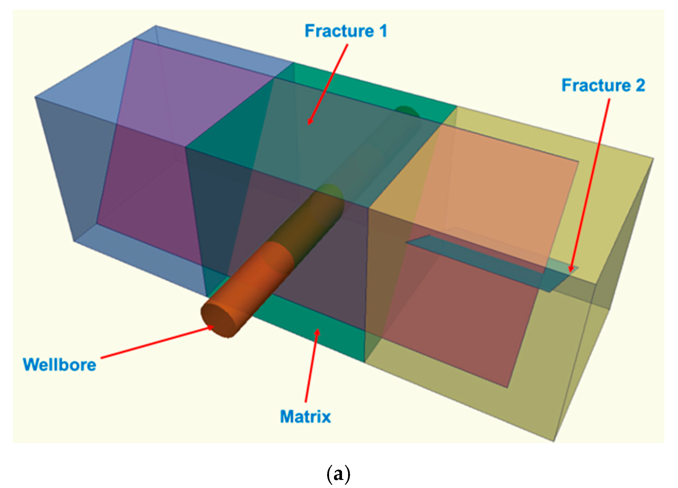
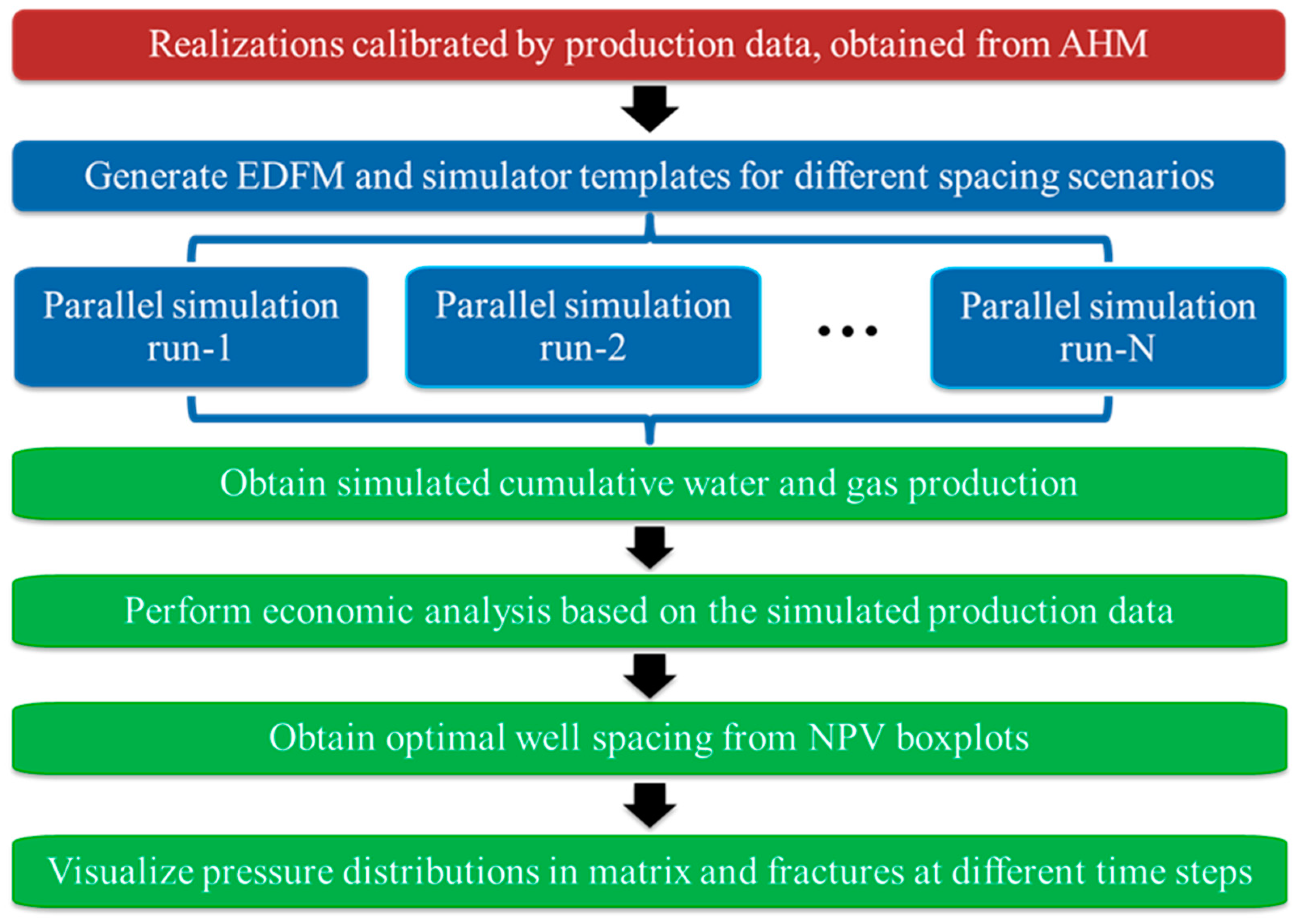
2. Methodology
3. Field Application in a Shale Gas Reservoir
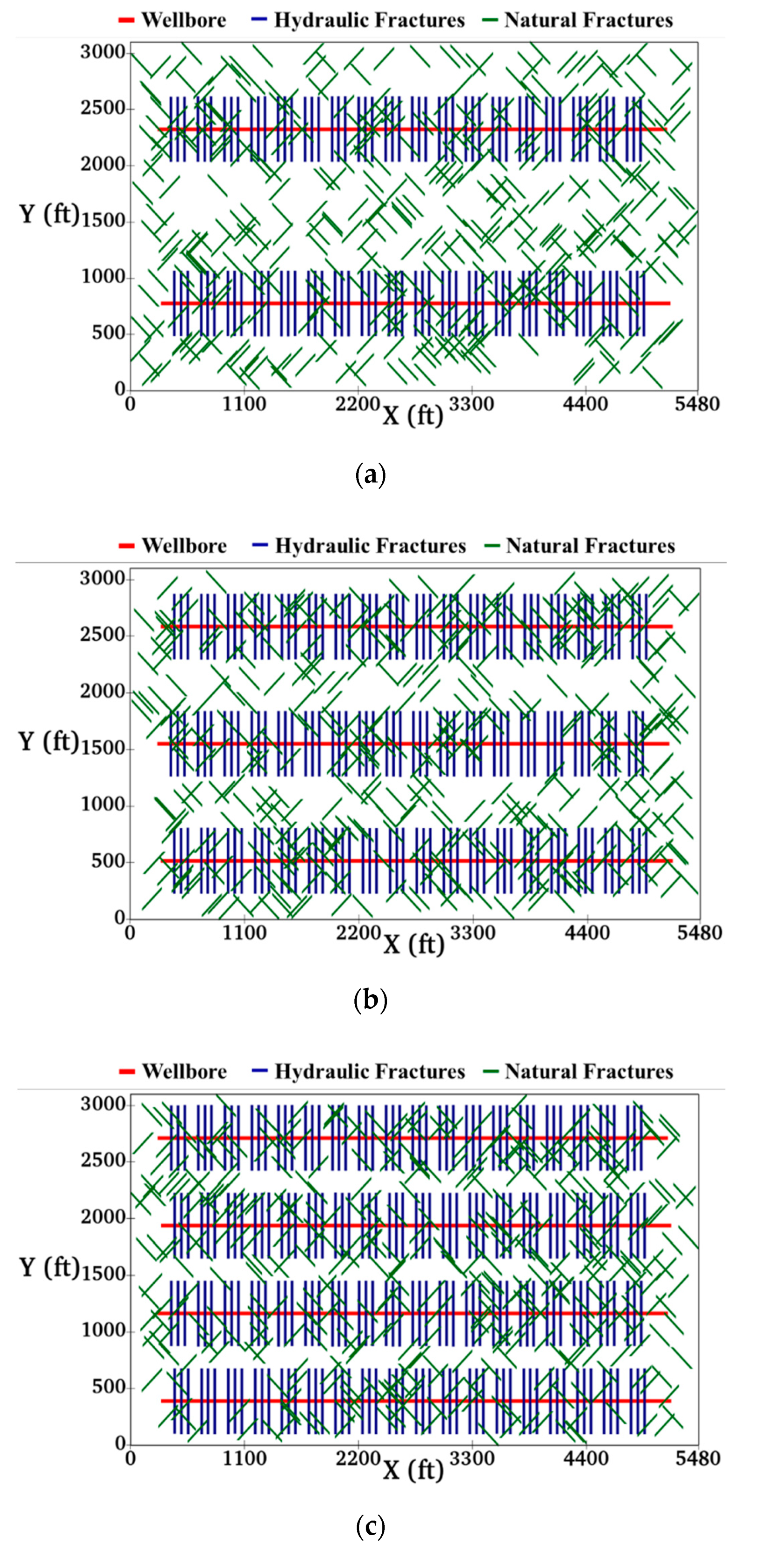
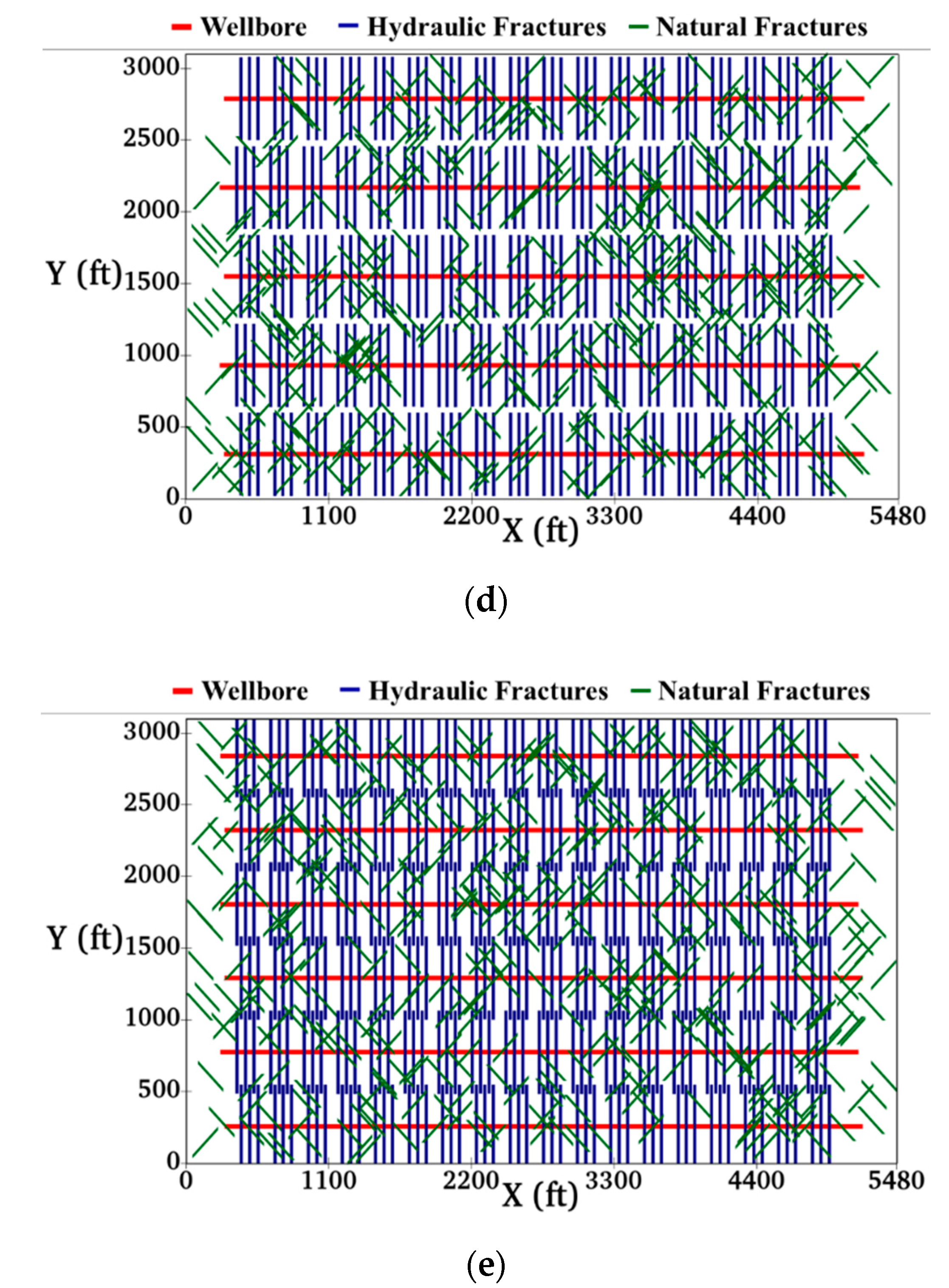
3.1. Reservoir Model
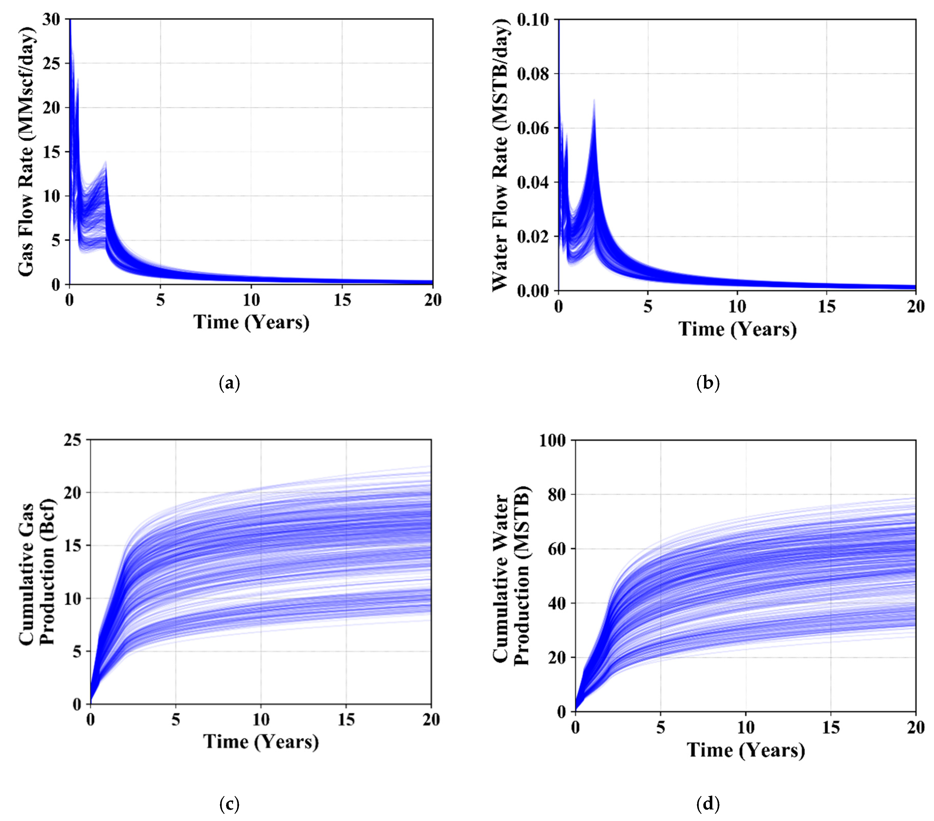
3.2. Simulation Results
3.3. Economic Analysis
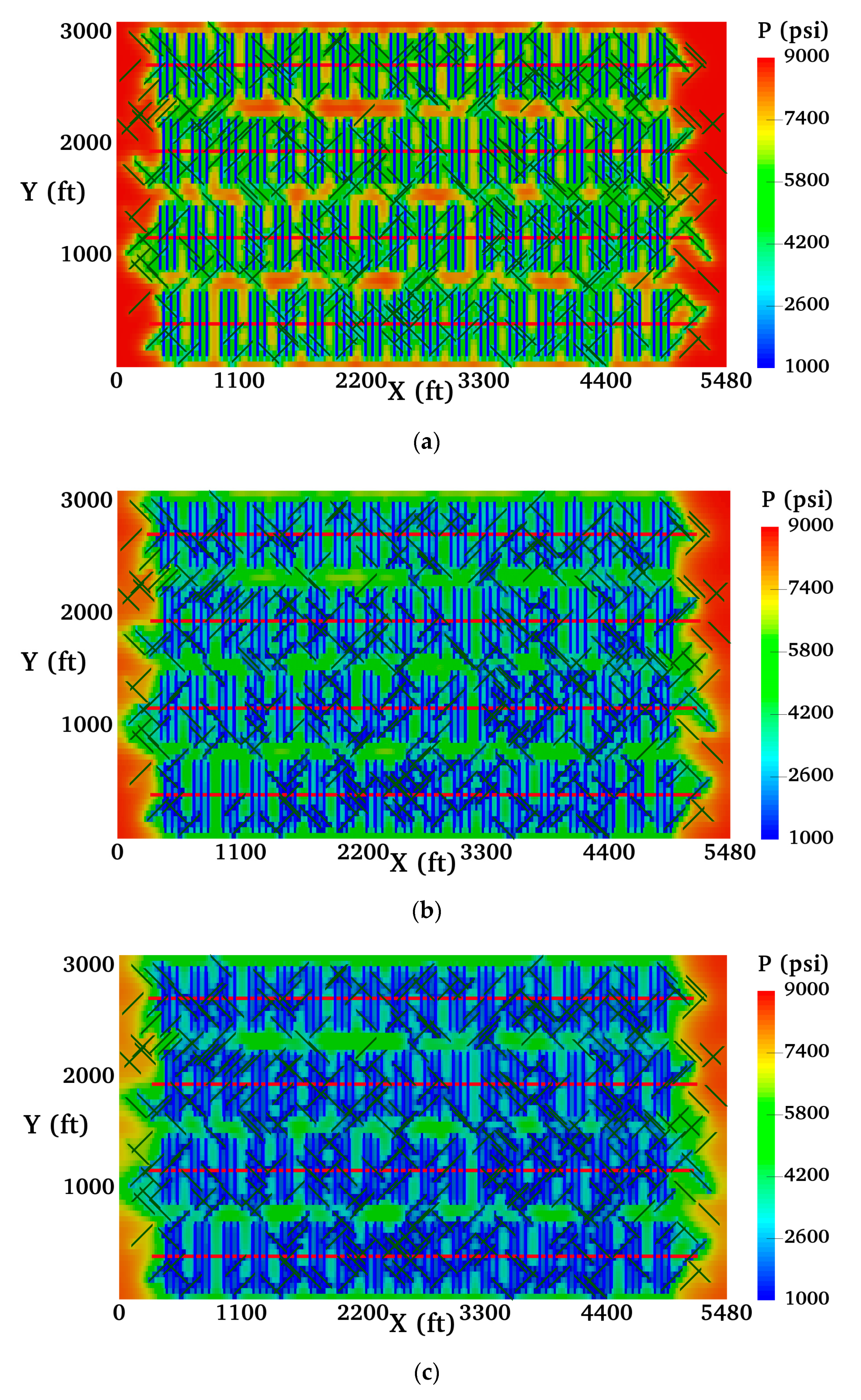
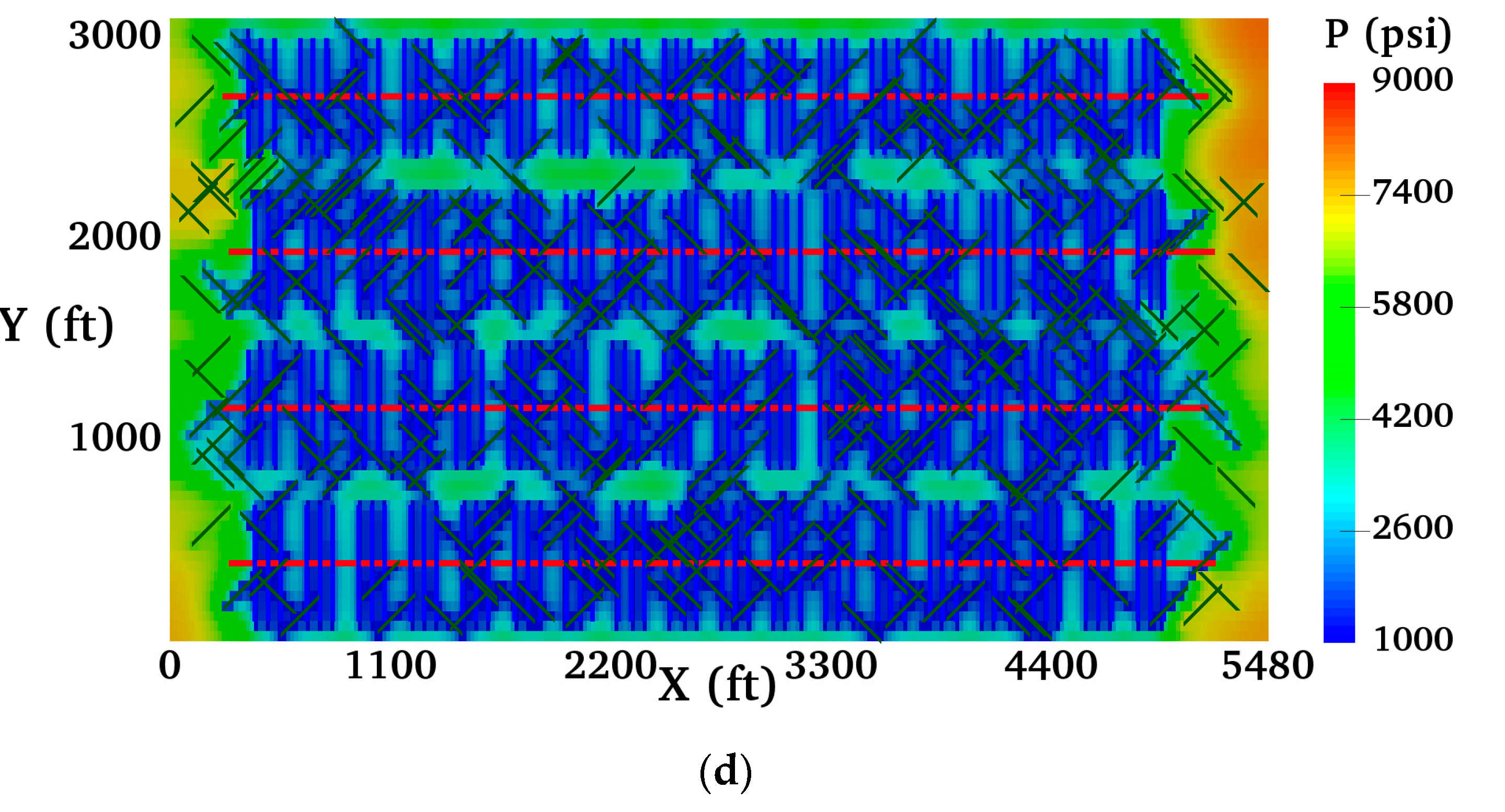
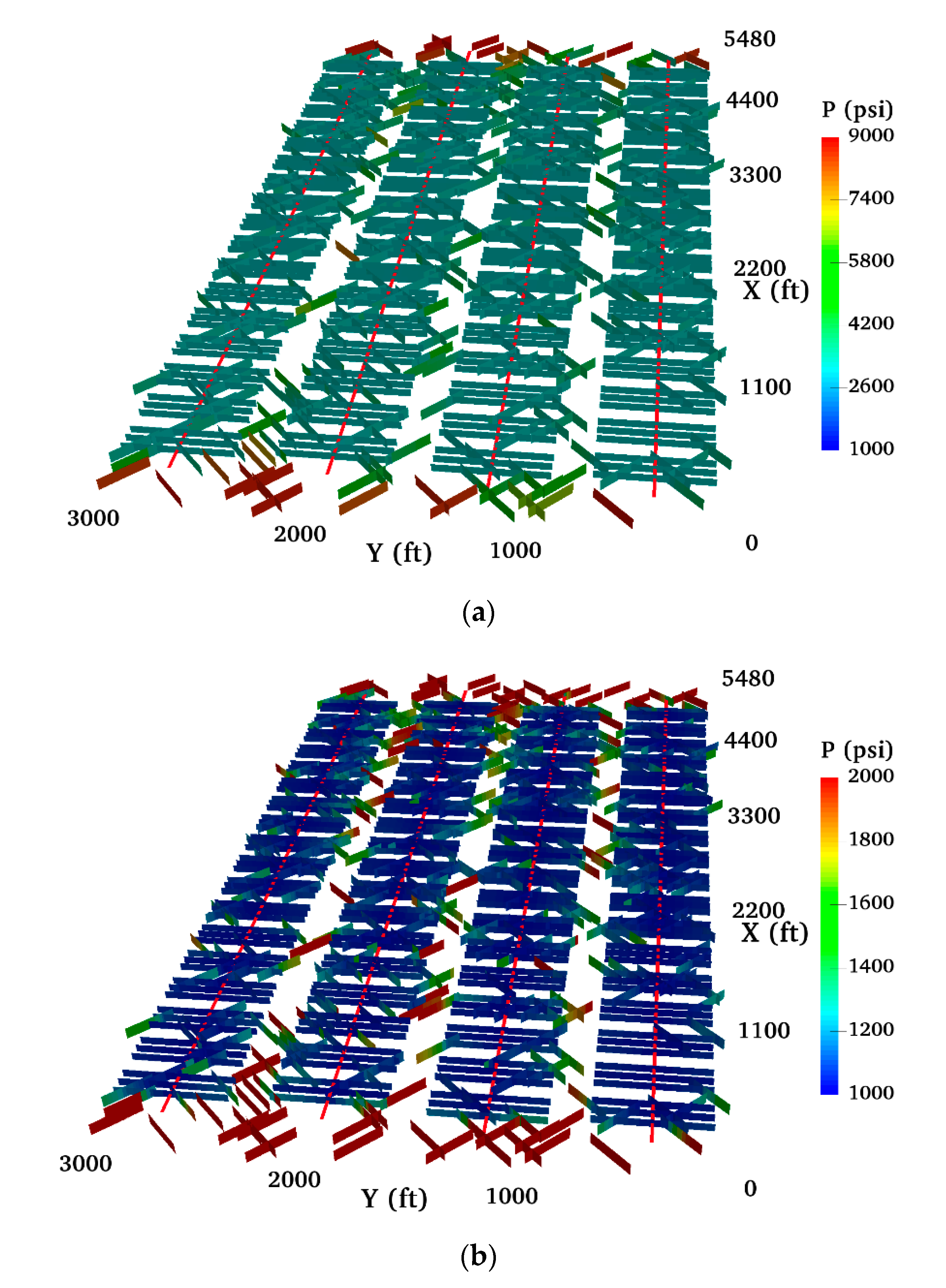
3.4. Pressure Visualizations
4. Conclusions
- (1)
- Well spacing can be optimized by designing well placement scenarios using multiple history matching solutions and by maximizing the calculated NPV. There exists a range of solutions that can improve the long-term project NPV for the well spacing optimization problem, so landing outside this solution range will jeopardize the economic performance.
- (2)
- The better the reservoir and fractures conditions (permeability, porosity, fracture half length, fracture height, etc.), then the higher the predictive NPV is. It would be substantially more beneficial if additional data can be gathered to build more realistic geological models (such as permeability/porosity map) of the reservoir.
- (3)
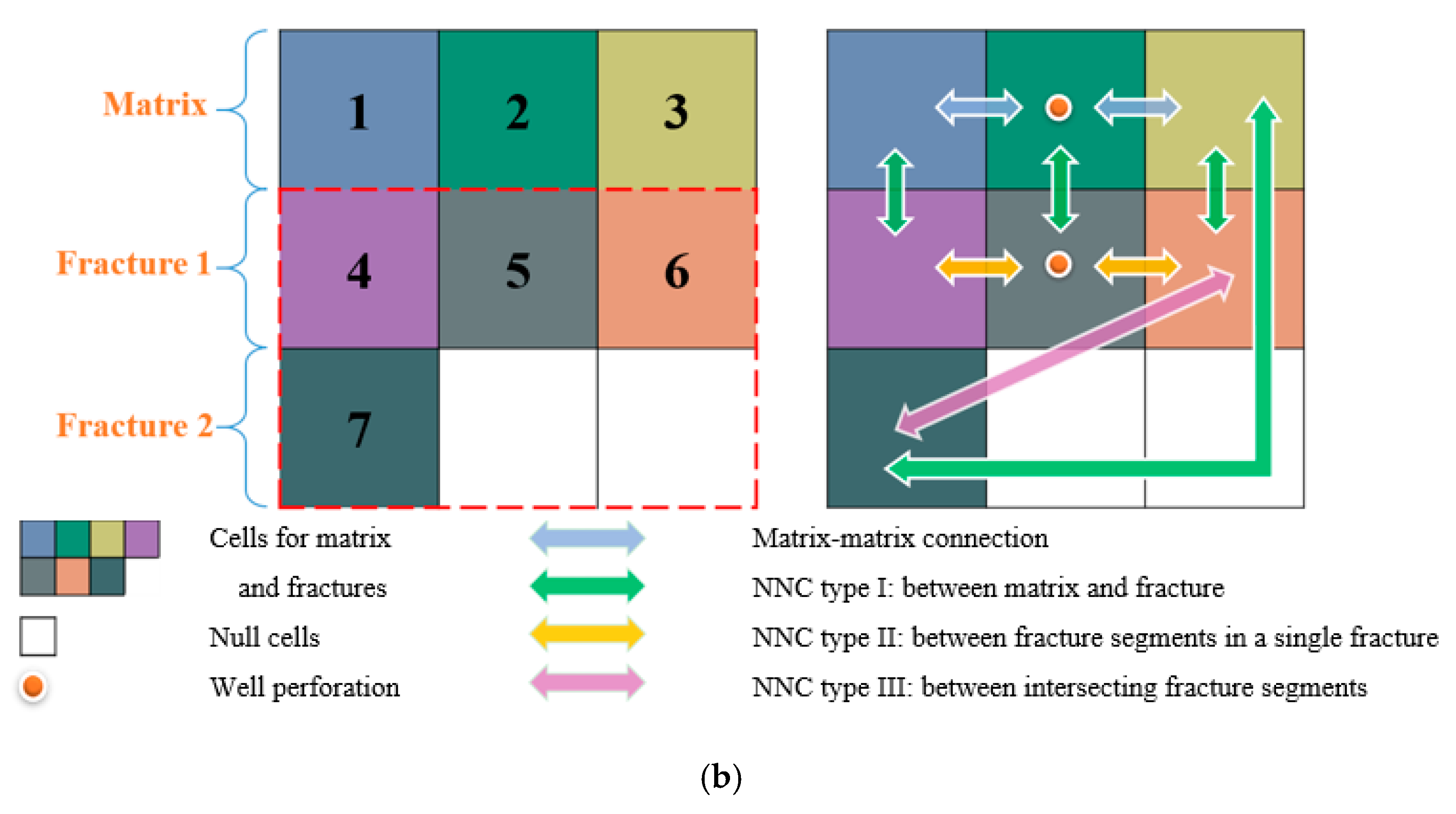
- The natural fractures that are near the wellbores contribute more to the total EUR and the economic performance than those that are not intersected with hydraulic fractures. However, the 2D modeling of the natural fractures are over simplified solutions, and more data (such as wellbore image log) should be acquired to accurately capture the spatial distributions of the network and to provide more insights regarding the well spacing problem.
- (4)
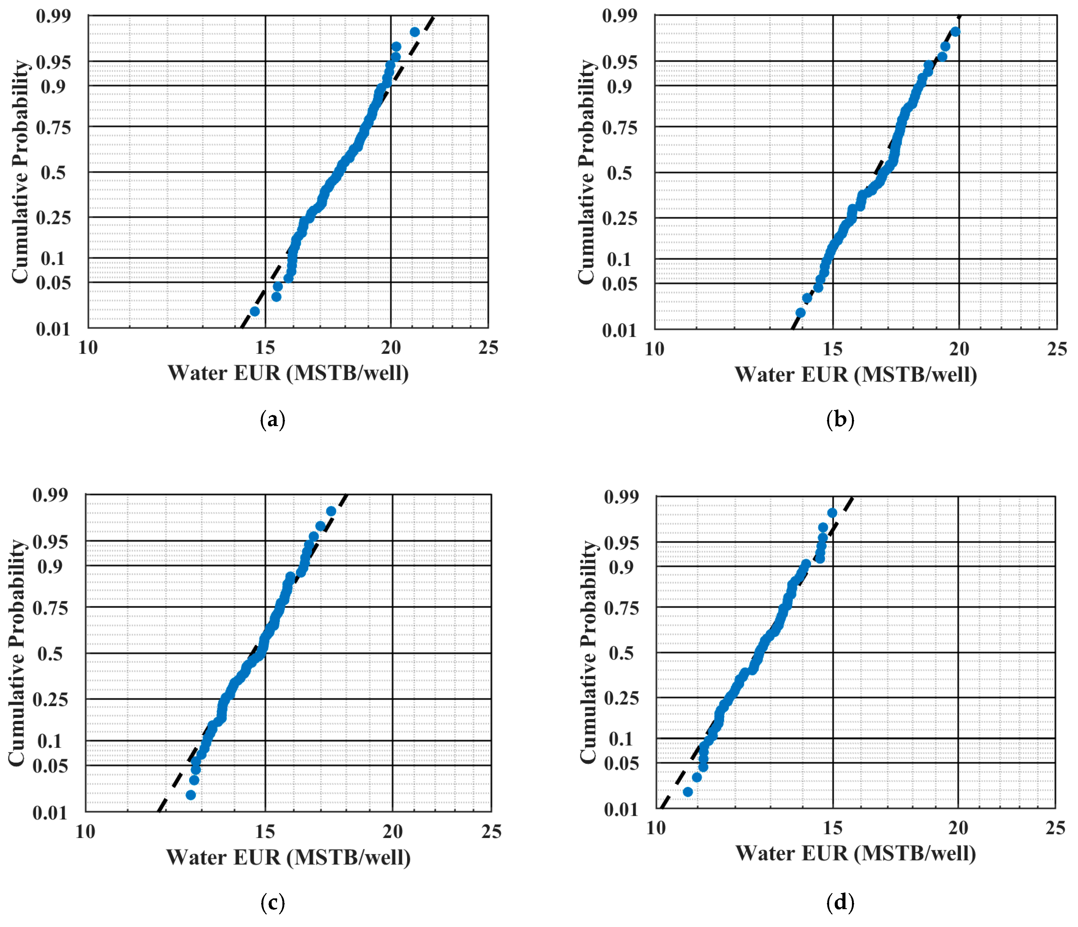
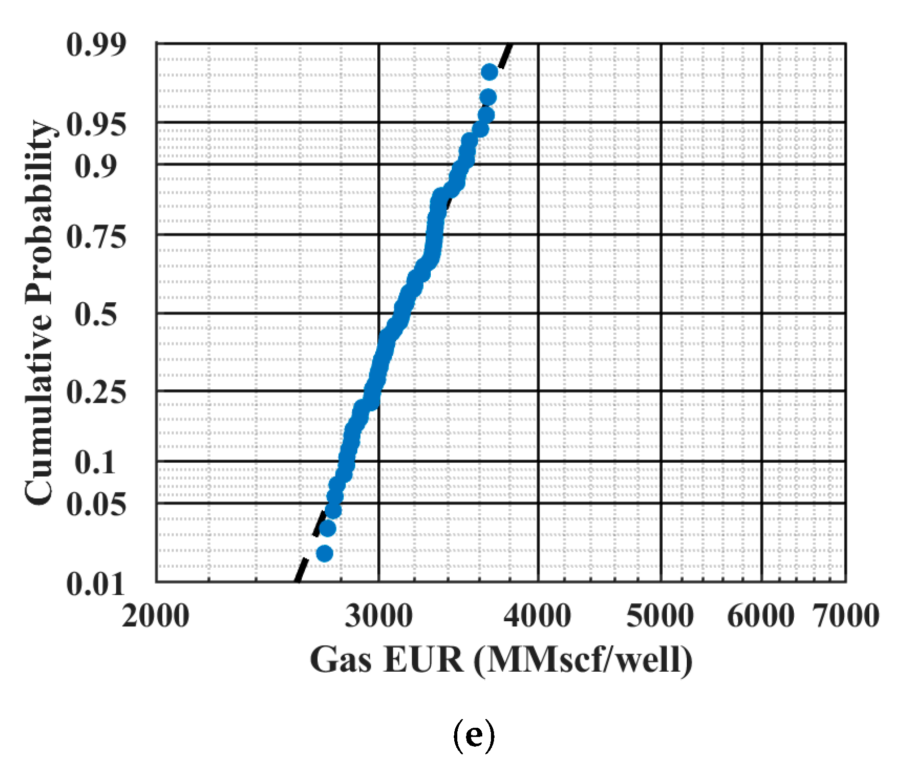
- The well spacing that maximizes the project NPV for this study is found to be approximately 236 m (775 ft), with 20-year gas EUR ranging from 101.9 to 135.9 Mm3 per well (3.6 to 4.8 Bcf per well) and 20 year water EUR ranging from 2.0 to 2.8 Km3 per well (12.5 to 17.5 MSTB per well). Nevertheless, more information regarding the hydraulic fractures’ geometry (using microseismic event data) might significantly affect the results obtained above.
- (5)
- For the NPV-maximizing well spacing outlined above, the project NPV ranges from 15 to 35 million dollars, with a P50 value of 25.9 million dollars.
Author Contributions
Funding
Acknowledgments
Conflicts of Interest
Abbreviations
| Abbreviation | Full Name |
| Bcf | Billion standard cubic feet |
| MMscf/Mm3 | Million standard cubic feet/ Million cubic meters |
| MPa | Mega pascal (106 pascal) |
| Mscf/Km3 | Thousand standard cubic feet/ Thousand cubic meters |
| MSTB | Thousand stock tank barrel |
References
- U.S. Energy Information Administration. Available online: https://www.eia.gov/todayinenergy/detail.php?id=11611 (accessed on 17 April 2020).
- Boulis, A.; Jayakumar, R.; Rai, R. A New Approach for Well Spacing Optimisation and Its Application to Various Shale Gas Resources. In Proceedings of the International Petroleum Technology Conference, Beijing, China, 26–28 March 2013. [Google Scholar] [CrossRef]
- Cao, R.; Li, R.; Girardi, A.; Chowdhury, N.; Chen, C. Well Interference and Optimum Well Spacing for Wolfcamp Development at Permian Basin. In Proceedings of the SPE/AAPG/SEG Unconventional Resources Technology Conference, Austin, TX, USA, 24–26 July 2017. [Google Scholar] [CrossRef]
- Iino, A.; Onishi, T.; Olalotiti-Lawal, F.; Datta-Gupta, A. Rapid Field-Scale Well Spacing Optimization in Tight and Shale Oil Reservoirs Using Fast Marching Method. In Proceedings of the SPE/AAPG/SEG Unconventional Resources Technology Conference, Houston, TX, USA, 23–25 July 2018. [Google Scholar] [CrossRef]
- Shandrygin, A. Optimization of Unconventional Gas Reservoirs Development by Horizontal Wells with Multiple Hydraulic Fracturing. In Proceedings of the SPE Russian Petroleum Technology Conference, Moscow, Russia, 22–24 October 2019. [Google Scholar] [CrossRef]
- Aniemena, C.; LaMarca, C.; Labryer, A. Well Spacing Optimization in Shale Reservoirs Using Rate Transient Analytics. In Proceedings of the SPE/AAPG/SEG Unconventional Resources Technology Conference, Denver, CO, USA, 22–24 July 2019. [Google Scholar] [CrossRef]
- Belyadi, H.; Yuyi, J.; Ahmad, M.; Wyatt, J. Deep Dry Utica Well Spacing Analysis with Case Study. In Proceedings of the SPE Eastern Regional Meeting, Canton, OH, USA, 13–15 September 2016. [Google Scholar] [CrossRef]
- Eburi, S.; Padmakar, A.S.; Wilson, K.; Banki, R.; Wardell, I. Well Spacing Optimization of Liquid Rich Shale Plays Using Reservoir Simulation. In Proceedings of the SPE Annual Technical Conference and Exhibition, Amsterdam, The Netherlands, 27–29 October 2014. [Google Scholar] [CrossRef]
- Liang, B.; Du, M.; Goloway, C.; Hammond, R.; Yanez, P.P.; Tran, T. Subsurface Well Spacing Optimization in the Permian Basin. In Proceedings of the SPE/AAPG/SEG Unconventional Resources Technology Conference, Austin, TX, USA, 24–26 July 2017. [Google Scholar] [CrossRef]
- Zhu, J.; Forrest, J.; Xiong, H.; Kianinejad, A. Cluster Spacing and Well Spacing Optimization Using Multi-Well Simulation for the Lower Spraberry Shale in Midland Basin. In Proceedings of the SPE Liquids-Rich Basins Conference, Midland, TX, USA, 13–14 September 2017. [Google Scholar] [CrossRef]
- Yu, W.; Sepehrnoori, K. Optimization of Well Spacing for Bakken Tight Oil Reservoirs. In Proceedings of the SPE/AAPG/SEG Unconventional Resources Technology Conference, Denver, CO, USA, 25–27 August 2014. [Google Scholar] [CrossRef]
- Grechka, V.; Li, Z.; Howell, B.; Garcia, H.; Wooltorton, T. Microseismic Imaging of Unconventional Reservoirs. In Proceedings of the SEG International Exposition and Annual Meeting, Anaheim, CA, USA, 14–19 October 2018. [Google Scholar] [CrossRef]
- Rafiee, M.; Grover, T. Well Spacing Optimization in Eagle Ford Shale: An Operator’s Experience. In Proceedings of the SPE/AAPG/SEG Unconventional Resources Technology Conference, Austin, TX, USA, 24–26 July 2017. [Google Scholar] [CrossRef]
- Ramanathan, V.; Boskovic, D.; Zhmodik, A.; Li, Q.; Ansarizadeh, M.; Perez Michi, O.; Garcia, G. A Simulation Approach to Modelling and Understanding Fracture Geometry with Respect to Well Spacing in Multi Well Pads in the Duvernay-A Case Study. In Proceedings of the SPE/CSUR Unconventional Resources Conference, Calgary, AB, Canada, 20–22 October 2015. [Google Scholar] [CrossRef]
- Suarez, M.; Pichon, S. Completion and Well Spacing Optimization for Horizontal Wells in Pad Development in the Vaca Muerta Shale. In Proceedings of the SPE Argentina Exploration and Production of Unconventional Resources Symposium, Buenos Aires, Argentina, 1–3 June 2016. [Google Scholar] [CrossRef]
- Weijermars, R.; Nandlal, K.; Khanal, A.; Tugan, M.F. Comparison of Pressure Front with Tracer Front Advance and Principal Flow Regimes in Hydraulically Fractured Wells in Unconventional Reservoirs. J. Pet. Sci. Eng. 2019, 183. [Google Scholar] [CrossRef]
- Weijermars, R.; Tugan, M.F.; Khanal, A. Production Rates and EUR Forecasts for Interfering Parent-Parent Wells and Parent-Child Wells: Fast Analytical Solutions and Validation with Numerical Reservoir Simulators. J. Pet. Sci. Eng. 2020, 190. [Google Scholar] [CrossRef]
- Hassen, R.A.; Fulford, D.S.; Burrows, C.T.; Starley, G.P. Decision-Focused Optimization: Asking the Right Questions About Well-Spacing. In Proceedings of the SPE Liquids-Rich Basins Conference, Midland, TX, USA, 5–6 September 2018. [Google Scholar] [CrossRef]
- John, M.-P.U.; Ibukun, S.; Pius, J.; Kayode, O. A Stochastic Approach to Well Spacing Optimization of Oil Reservoirs. In Proceedings of the Nigeria Annual International Conference and Exhibition, Abuja, Nigeria, 30 July–3 August 2011. [Google Scholar] [CrossRef]
- Al-Rukabi, M.; Forouzanfar, F. Application of Assisted History Matching to Unconventional Assets. In Proceedings of the SPE Annual Technical Conference and Exhibition, Calgary, AB, Canada, 30 September–2 October 2019. [Google Scholar] [CrossRef]
- Lind, R.H.; Allottai, O.; Gaaim, A.M.; Almuallim, H. Computer Assisted History Matching-A Field Example. In Proceedings of the SPE Reservoir Characterization and Simulation Conference and Exhibition, Abu Dhabi, UAE, 16–18 September 2013. [Google Scholar] [CrossRef]
- Shams, M. Reservoir Simulation Assisted History Matching: From Theory to Design. In Proceedings of the SPE Kingdom of Saudi Arabia Annual Technical Symposium and Exhibition, Dammam, Saudi Arabia, 25–28 April 2016. [Google Scholar] [CrossRef]
- Ma, X.; Gupta, A.D.; Efendiev, Y. A Multistage MCMC Method with Nonparametric Error Model for Efficient Uncertainty Quantification in History Matching. In Proceedings of the SPE Annual Technical Conference and Exhibition, Denver, CO, USA, 21–24 September 2008. [Google Scholar] [CrossRef]
- Tripoppoom, S.; Yu, W.; Sepehrnoori, K.; Miao, J. Application of Assisted History Matching Workflow to Shale Gas Well Using EDFM and Neural Network-Markov Chain Monte Carlo Algorithm. In Proceedings of the Unconventional Resources Technology Conference, Denver, CO, USA, 22–24 July 2019. [Google Scholar] [CrossRef]
- Xu, Y.; Cavalcante Filho, J.S.A.; Yu, W.; Sepehrnoori, K. Discrete-fracture modeling of complex hydraulic-fracture geometries in reservoir simulators. SPE Reserv. Eval. Eng. 2017, 20, 403–422. [Google Scholar] [CrossRef]
- Xu, Y.; Yu, W.; Sepehrnoori, K. Modeling Dynamic Behaviors of Complex Fractures in Conventional Reservoir Simulators. In Proceedings of the SPE/AAPG/SEG Unconventional Resources Technology Conference, Austin, TX, USA, 24–26 July 2017. [Google Scholar] [CrossRef]
- Xu, Y.; Yu, W.; Li, N.; Lolon, E.; Sepehrnoori, K. Modeling Well Performance in Piceance Basin Niobrara Formation using Embedded Discrete Fracture Model. In Proceedings of the SPE/AAPG/SEG Unconventional Resources Technology Conference, Houston, TX, USA, 23–25 July 2018. [Google Scholar] [CrossRef]
- Langmuir, I. The Adsorption of Gases on Plane Surfaces of Glass, Mica and Platinum. J. Am. Chem. Soc. 1918, 40, 1403–1461. [Google Scholar] [CrossRef] [Green Version]


| Reservoir Description | Value | Unit |
|---|---|---|
| Model dimensions (x × y × z) | 1670 × 945 × 20 (5480 × 3100 × 65) | m (ft) |
| Number of grid blocks (x × y × z) | 137 × 31 × 1 | - |
| Grid block dimension (x × y × z) | 12.2 × 30.5 × 65 (40 × 100 × 65) | m (ft) |
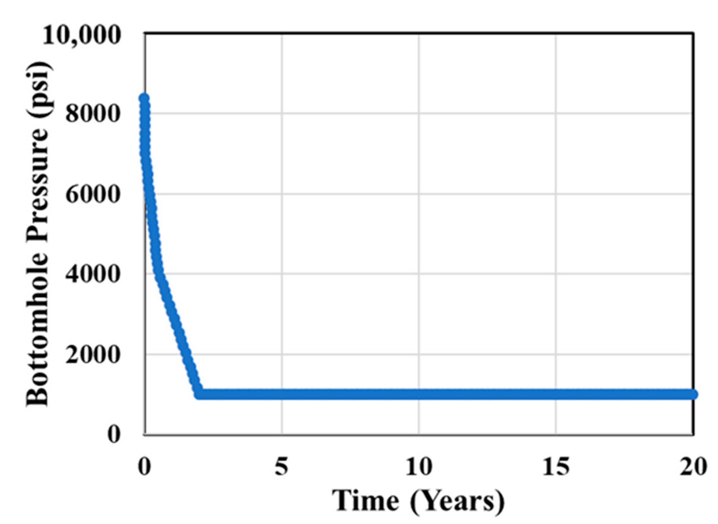
| Initial reservoir pressure | 61 (8847.3) | MPa (psi) |
| Reservoir temperature | 102 (215) | () |
| Residual water saturation | 20% | - |
| Residual gas saturation | 10% | - |
| Initial water saturation | 39% | - |
| Initial gas saturation | 61% | - |
| Total compressibility | 4.35 × 10⁻⁴ (3 × 10⁻⁶) | MPa−1 (psi−1) |
| Reservoir depth | 3200 (10,499) | m (ft) |
| Well length | 1500 (4921) | m (ft) |
| Number of stages | 18 | - |
| Stage spacing | 44 (145) | m (ft) |
| Clusters per stage | 3 | - |
| Cluster spacing | 20.4 (67) | m (ft) |
| Uncertain Parameters | Unit | Minimum Value | Maximum Value |
|---|---|---|---|
| Matrix permeability | nd | 27 | 937 |
| Fracture half length | m (ft) | 61 (200) | 133.2 (437) |
| Fracture height | m (ft) | 7.62 (25) | 19.8 (65) |
| Fracture conductivity | md-m (md-ft) | 9.1 (30) | 60.7 (199) |
| Fracture water saturation | % | 56 | 90 |
| Fracture width | m (ft) | 0.03 (0.1) | 0.287 (0.94) |
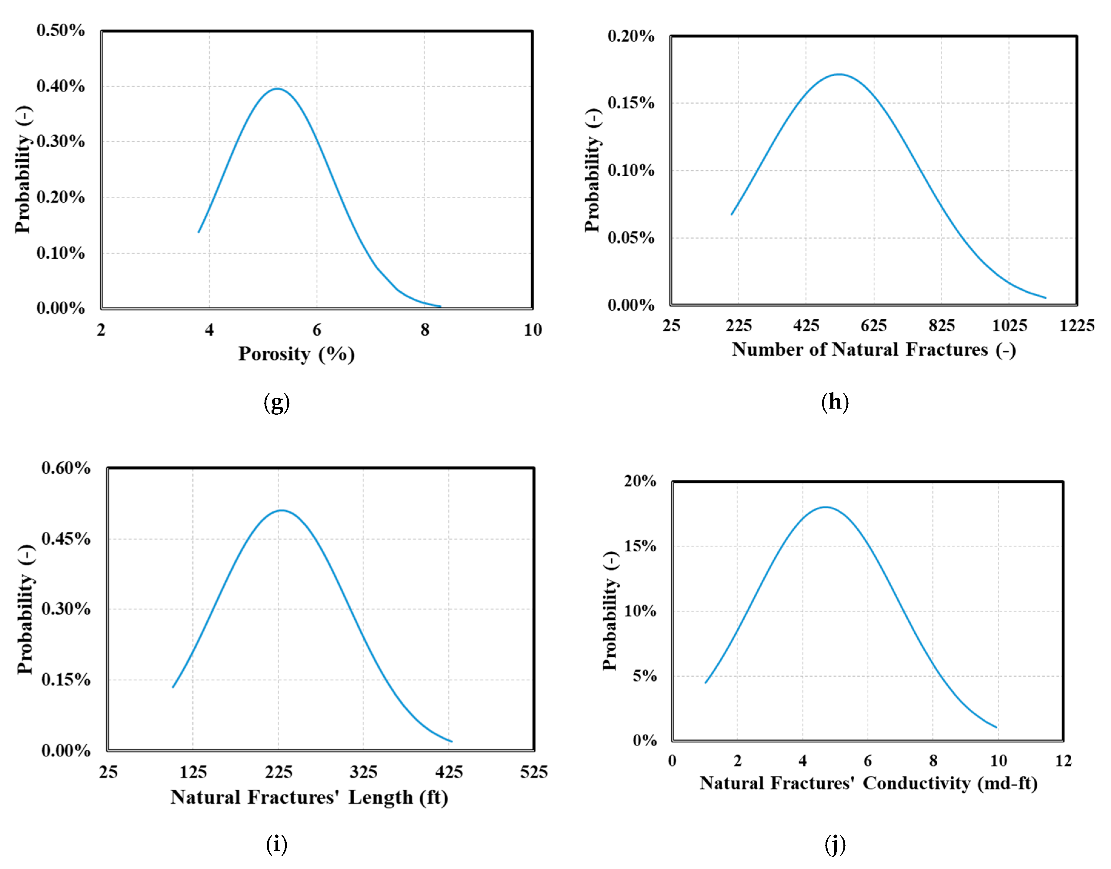
| Matrix porosity | % | 3.8 | 8.3 |
| Number of natural fractures | - | 205 | 1132 |
| Natural fractures’ length | m (ft) | 30.8 (101) | 130.5 (428) |
| Natural fractures’ conductivity | md-m (md-ft) | 0.3 (1) | 3.05 (10) |
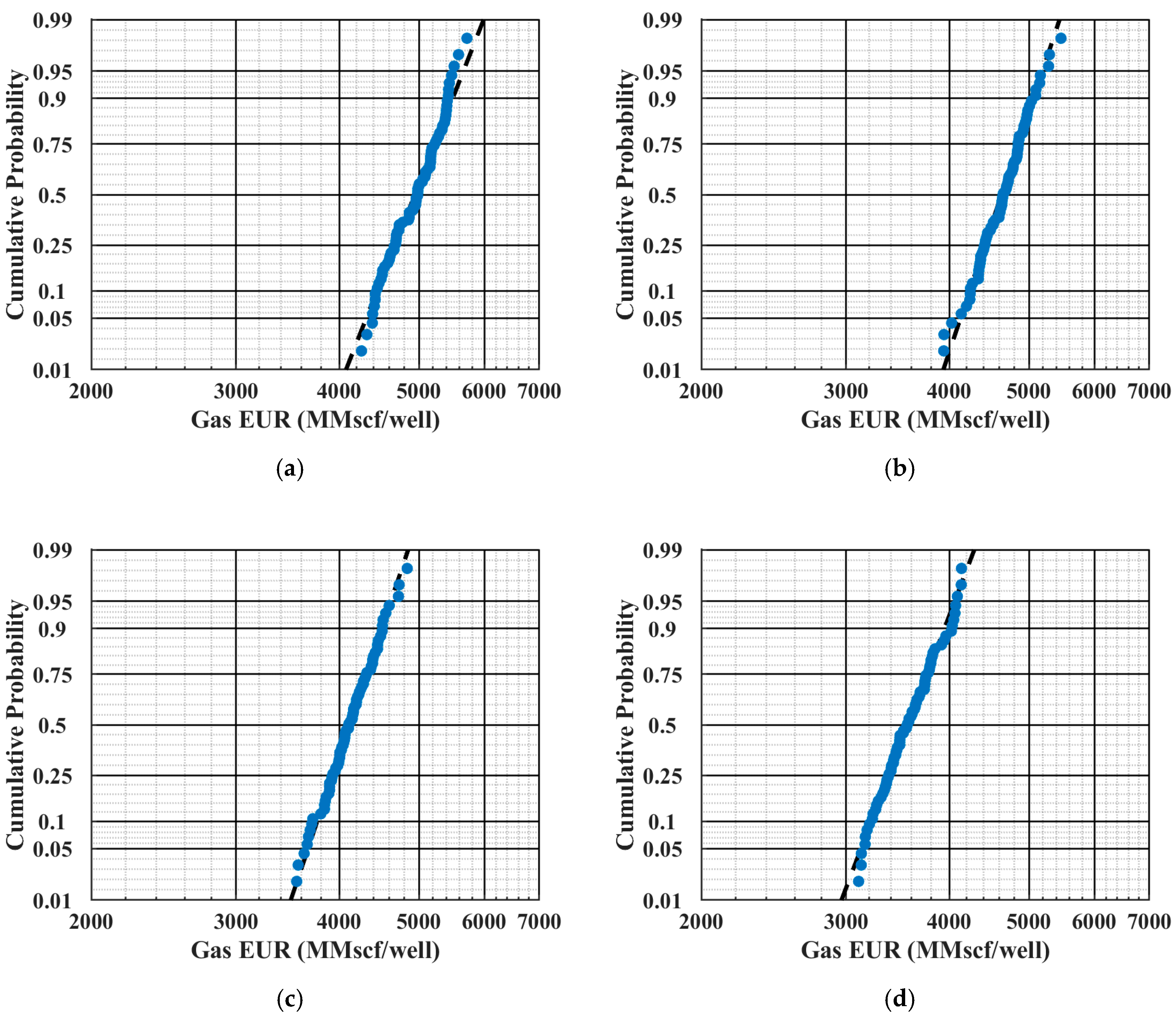
| Spacing Scenario | Gas EUR P10 Mm3/Well (MMscf/Well) | Gas EUR P50 Mm3/Well (MMscf/Well) | Gas EUR P90 Mm3/Well (MMscf/Well) | Water EUR P10 Km3/Well (MSTB/Well) | Water EUR P50 Km3/Well (MSTB/Well) | Water EUR P90 Km3/Well (MSTB/Well) |
|---|---|---|---|---|---|---|
| 2 wells | 125.4 (4430) | 141.3 (4990) | 155.7 (5500) | 2.53 (15.8) | 2.83 (17.7) | 3.2 (20) |
| 3 wells | 119.5 (4220) | 131.7 (4650) | 142.3 (5025) | 2.37 (14.8) | 2.64 (16.5) | 2.91 (18.2) |
| 4 wells | 106.8 (3770) | 116 (4100) | 127.4 (4500) | 2.08 (13) | 2.34 (14.6) | 2.62 (16.4) |
| 5 wells | 90.6 (3200) | 101.4 (3580) | 111.9 (3950) | 1.79 (11.2) | 2.03 (12.7) | 2.27 (14.2) |
| 6 wells | 79.9 (2820) | 89.5 (3160) | 99.1 (3500) | 1.49 (9.3) | 1.78 (11.1) | 2.0 (12.5) |
| Spacing Scenario | Gas EUR P50 Change Mm3/Well (MMscf/Well) | Water EUR P50 Change Km3/Well (MSTB/Well) |
|---|---|---|
| 2 wells to 3 wells | −9.6 (−340) | −0.19 (−1.2) |
| 3 wells to 4 wells | −15.7 (−550) | −0.30 (−1.9) |
| 4 wells to 5 wells | −14.6 (−520) | −0.31 (−1.9) |
| 5 wells to 6 wells | −11.9 (−420) | −0.25 (−1.6) |
| Spacing Scenario | NPV P25 | NPV P50 | NPV P75 |
|---|---|---|---|
| Million Dollars | Million Dollars | Million Dollars | |
| 2 wells | 15 | 17.5 | 18.7 |
| 3 wells | 20.5 | 22.8 | 24.9 |
| 4 wells | 22.7 | 25.9 | 27.8 |
| 5 wells | 19.5 | 22.5 | 25.7 |
| 6 wells | 14.2 | 19.0 | 22.1 |
© 2020 by the authors. Licensee MDPI, Basel, Switzerland. This article is an open access article distributed under the terms and conditions of the Creative Commons Attribution (CC BY) license (http://creativecommons.org/licenses/by/4.0/).
Share and Cite
Chang, C.; Liu, C.; Li, Y.; Li, X.; Yu, W.; Miao, J.; Sepehrnoori, K. A Novel Optimization Workflow Coupling Statistics-Based Methods to Determine Optimal Well Spacing and Economics in Shale Gas Reservoir with Complex Natural Fractures. Energies 2020, 13, 3965. https://doi.org/10.3390/en13153965
Chang C, Liu C, Li Y, Li X, Yu W, Miao J, Sepehrnoori K. A Novel Optimization Workflow Coupling Statistics-Based Methods to Determine Optimal Well Spacing and Economics in Shale Gas Reservoir with Complex Natural Fractures. Energies. 2020; 13(15):3965. https://doi.org/10.3390/en13153965
Chicago/Turabian StyleChang, Cheng, Chuxi Liu, Yongming Li, Xiaoping Li, Wei Yu, Jijun Miao, and Kamy Sepehrnoori. 2020. "A Novel Optimization Workflow Coupling Statistics-Based Methods to Determine Optimal Well Spacing and Economics in Shale Gas Reservoir with Complex Natural Fractures" Energies 13, no. 15: 3965. https://doi.org/10.3390/en13153965