Article

Uncertainty Quantification of the Effects of Blade Damage on the Actual Energy Production of Modern Wind Turbines

1
Department of Industrial Engineering, Università degli Studi di Firenze, 50139 Florence, Italy
2
Department of Engineering, Lancaster University, Lancaster LA1 4YW, UK
3
Department of Energy, Politecnico di Torino, 10129 Torino, Italy
4
Department of Mechanical Engineering, University of Bath, Bath BA2 7AY, UK
*
Author to whom correspondence should be addressed.
Energies 2020, 13(15), 3785; https://doi.org/10.3390/en13153785
Submission received: 30 June 2020 / Revised: 21 July 2020 / Accepted: 22 July 2020 / Published: 23 July 2020
(This article belongs to the Special Issue Numerical Simulation of Wind Turbines)

Abstract

:
Wind turbine blade deterioration issues have come to the attention of researchers and manufacturers due to the relevant impact they can have on the actual annual energy production (AEP). Research has shown how after prolonged exposure to hail, rain, insects or other abrasive particles, the outer surface of wind turbine blades deteriorates. This leads to increased surface roughness and material loss. The trailing edge (TE) of the blade is also often damaged during assembly and transportation according to industry veterans. This study aims at investigating the loss of AEP and efficiency of modern multi-MW wind turbines due to such issues using uncertainty quantification. Such an approach is justified by the stochastic and widely different environmental conditions in which wind turbines are installed. These cause uncertainties regarding the blade’s conditions. To this end, the test case selected for the study is the DTU 10 MW reference wind turbine (RWT), a modern reference turbine with a rated power of 10 MW. Blade damage is modelled through shape modification of the turbine’s airfoils. This is done with a purposely developed numerical tool. Lift and drag coefficients for the damaged airfoils are calculated using computational fluid dynamics. The resulting lift and drag coefficients are used in an aero-servo-elastic model of the wind turbine using NREL’s code OpenFAST. An arbitrary polynomial chaos expansion method is used to estimate the probability distributions of AEP and power output of the model when blade damage is present. Average AEP losses of around 1% are predicted mainly due to leading-edge blade damage. Results show that the proposed method is able to account for the uncertainties and to give more meaningful information with respect to the simulation of a single test case.

Graphical Abstract

1. Introduction

Wind turbine damage has in recent years gained interest from industry and academia in an effort to keep aging wind parks around the globe productive. According to Rempel [1], in the early days of the wind energy industry there was the general misconception that once the blade is in operation, no further maintenance is required. This has changed, partly due to a considerable number of field reports that have started to surface in recent years highlighting extreme and worrying examples of early blade deterioration. For instance, Rempel states that blades as young as three years of age can show signs of wear and that blades of 87 out of 111 wind turbines in a wind farm off the shores of Denmark had to be dismantled and brought to shore after less than five years in operation due to severe leading-edge (LE) damage, as shown in Røndgaard [2].
In addition to the more common LE issues, blade’s trailing edge often suffers from damage. In particular, Decoret [3] states that debonding is commonly observed at the trailing edge (TE). This phenomenon occurs when the composite layers of the blade shell separate. If this happens at the TE of the blade, its dimension is expected to greatly increase in thickness, thus decreasing the aerodynamic performance. According to Wood [4], another common source of damage at the TE happens during blade transportation and turbine assembly. Crushing of the laminate may occur as well as chipping of the TE itself, especially in the tip region where the rear of the blades is typically very thin. The impact of LE damage on AEP has been studied by various authors. Amongst the most influential research in the field, Sareen et al. [5] test in a wind-tunnel a series of LE-damaged wind turbine airfoil configurations that mimic pictures of blades that were brought in for repair. They predict massive maximum losses in AEP of up to 25%. Han et al. [6] develop a computational fluid dynamics (CFD) model of an eroded airfoil based on their inspection of a 14-year-old Vestas V47 blade using the commercial software Star CCM+. They then simulate the NREL 5 MW [7] rotor with erosion applied from 70.7% of the rotor span outwards and find AEP reductions of 3.7%. Castorrini et al. [8] develop a numerical tool to predict airfoil performance degradation due to LE erosion. The tool is tuned based on photographic evidence of damaged blades and tested on the NREL 5 MW rotor, predicting power decreases of around 8%. As also noted by Herring et al. [9], these values, and others that can be found in published literature, quantitively greatly differ between each other. This could be due to the fact that erosion has a variable impact on different airfoil shapes, turbine sizes and operating conditions, thus leading to different results. Moreover, as far as the authors are aware, no study assesses the impact of TE damage on AEP at the present time, while some of the authors recently analyzed its effects on aerodynamic performance and loads under realistic inflow conditions [10]. Some light can be shed on the discrepancies highlighted between the work of many authors by approaching the problem in a probabilistic manner rather than in a deterministic way, as done until now.
This is done in the present study by introducing two aleatory variables that model leading-edge and trailing-edge damage, respectively. That blade damage is propagated through an aero-servo-elastic model of the DTU 10 MW RWT [11] as this is a modern reference rotor design. The model response in terms of AEP and power is approximated using an arbitrary polynomial chaos (aPC) expansion. The numerical procedure that is followed will be detailed in the following sections; however, a brief rundown can be provided as follows. The damage is applied to a give airfoil through geometry modification. The lift and drag coefficients are then obtained using computational fluid dynamics (CFD). The obtained coefficients are applied to the DTU10MW blade. The turbine is then simulated using NREL’s open-source code OpenFAST [12]. Finally, the model regression can be performed and response surfaces of the outputs of interest, as well as associated probability density functions (PDFs), can be estimated. An overview of the entire modelling process is provided in Figure 1.
It should be noted that blade damage is undoubtedly not the only source of uncertainty that affects the power production of a wind farm. Other common sources of uncertainty are related to environmental conditions, with uncertainties in wind speed and turbulence intensity being the main ones. As these are not the topic of the present study, which focuses specifically on the effects of blade damage, they are not included in the uncertainty quantification; however, in order to ensure that the study is up to the present simulation standards, they are accounted for using the standard procedures of the International Electrotechnical Commission (IEC).

2. Materials and Methods

In this section, the main details regarding the numerical modelling tools and choices that were made are given. Firstly, the numerical methods used to estimate the uncertainty associated to blade damage are introduced. The hypotheses regarding the input uncertainties are then explained. Finally, in the following subsections the numerical tools used in the required deterministic model evaluations are detailed.

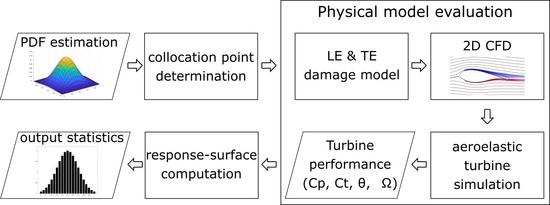
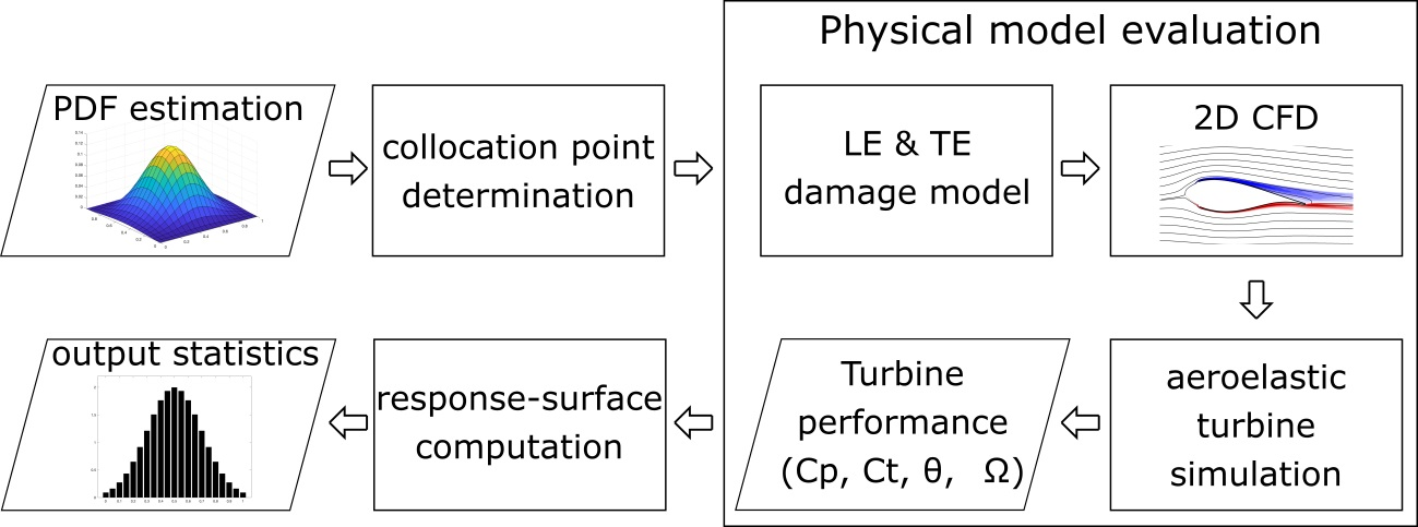
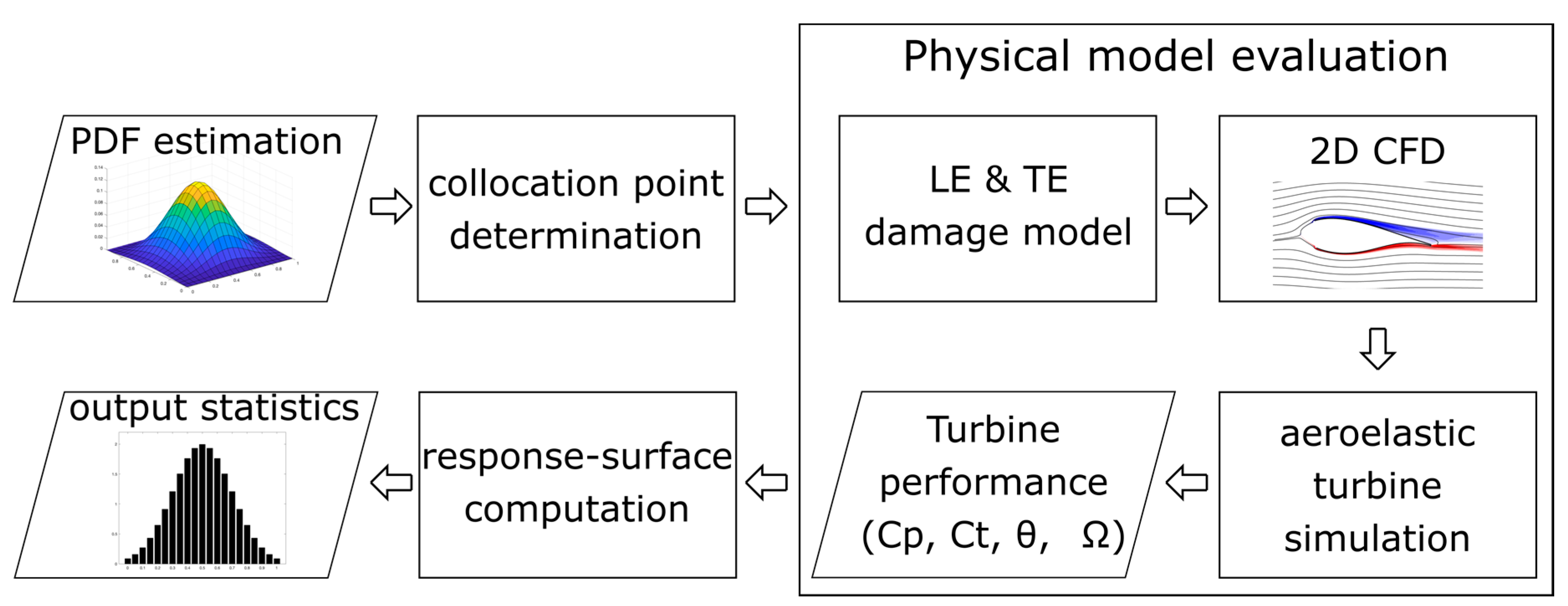
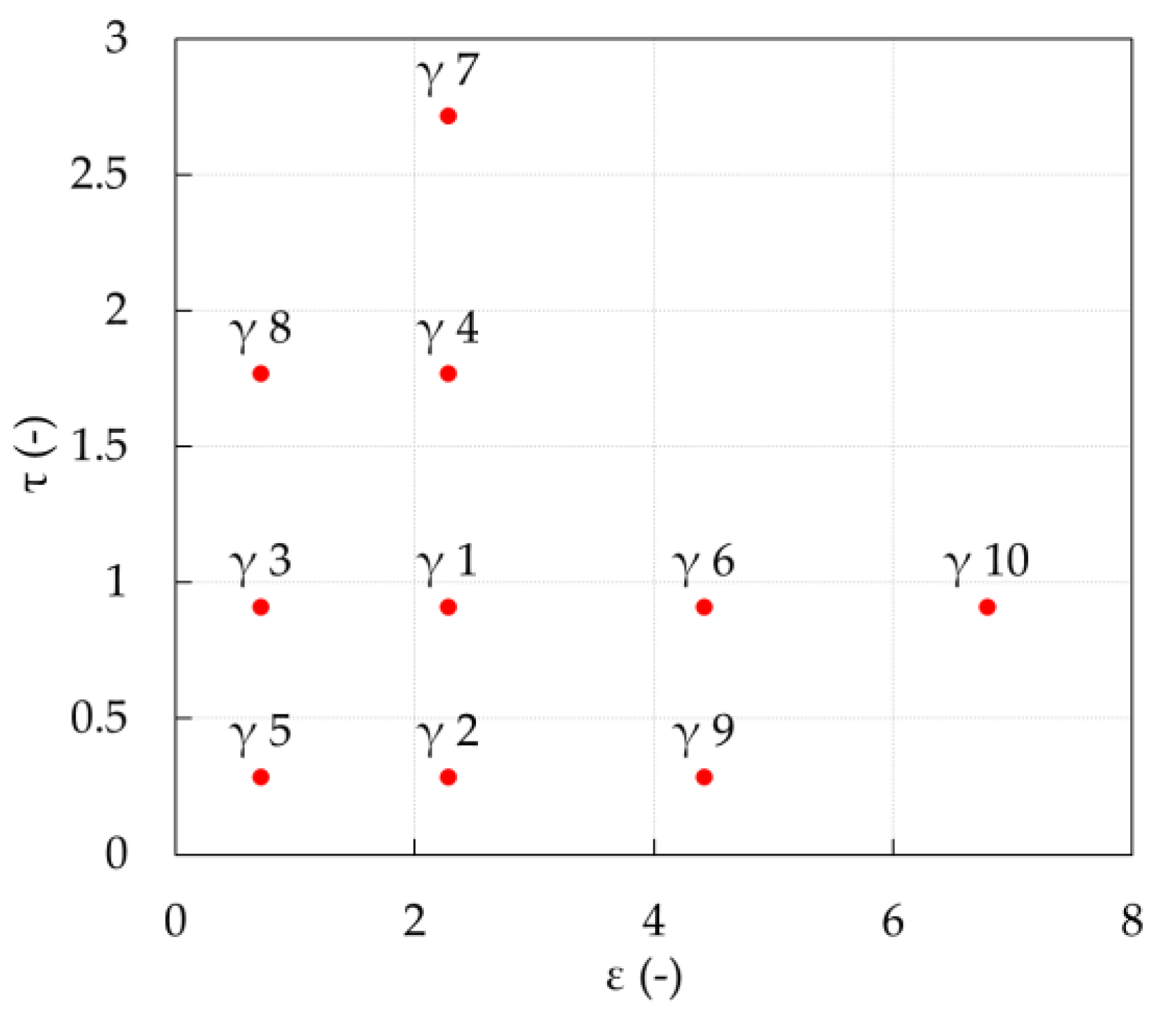
2.1. Stochastic Approach

The stochastic approach exploited in the present work falls into the class of the arbitrary polynomial chaos (aPC) as implemented by Oladyshkin and Novak [13]. This technique falls into the field of the study of aleatory uncertainty, which only accounts for deviations of boundary condition and geometrical parameters. The present approach does not include the contribution of the limits of the numerical approach adopted. The deviation or the effect of such limitation have been considered as negligible. CFD has been validated and run according to best practices, including grid independence study. This approach has the advantage of providing stochastic results (or PDFs) without the need to change the algorithm of the numerical tools employed in the simulations. These kinds of approaches are generally known as non-invasive methods as reviewed by Iaccarino [14] and more detailed in Carnevale [15] and Ahfield [16]. The PDF of a specific quantity of interest is extracted by reproducing a surface response obtained by a certain number of simulations (or deterministic realization). The boundary conditions for these simulations are set to reproduce the PDF representing the aleatory parameter. The process of selecting appropriate boundary conditions is known as sampling. The sampling process is usually obtained by means of selecting the boundary condition using the Monte Carlo method filtered by the proper PDF. The approach as described implies a large number of simulations and it is not reliable for application where CFD solvers are used for each single deterministic prediction. This would require a high computational cost to complete the simulation campaign.
A strategy to overcome this limitation consists of a clever choice of the boundary conditions resulting in a limited number of simulations. The convolution of this boundary conditions is representative of a specific PDF. This approach is known in literature as the probabilistic collocation point (PCM). The PCM are obtained as quadrature points of a linear system built on the basis consisting in a set of polynomials (polynomial chaos, PC). The choice of these polynomials corresponds to make a strong assumption on how the response surface is determined. The surface response will be as the weighted functions corresponding to a specific PDF. Mathematic foundations can be found in Tatang et al. [17]. This particular approach has been successfully applied to CFD simulations in Carnevale et al. [15,18] and Salvadori et al. [19]. The particular approach proposed allows weaker hypothesis to be considered on the PDF of the aleatory parameter. The aPC only demands the existence of a finite number of moments and does not require the complete knowledge or even the existence of a probability density function. This approach has also been employed in Ahlfield et al. [16], where the stochastic behavior physical parameters are characterized by discontinuity and Gibbs phenomena. The aPC extends chaos expansion techniques by employing a global polynomial basis.
Let’s consider a generic aleatory variable ξ propagating on a specific output of interest Y = f ( ξ ) , where f is a general unknown stochastic model (or PDF); it can be expressed as a d-order expansion:
Y ( ξ ) i = 1 d c i P ( i ) ( ξ )
According to the general theory of PCM the characteristic statistical quantities of Y ( ξ ) can be evaluated by the coefficient c i , and the momentum and variance are expressed as follows:
μ Y = c 1 , σ Y 2 = i = 1 d c i
The peculiarity of the aPC approach is related to the strategy adopted to determine the orthonormal basis of polynomial P ( i ) . These polynomials have been determined by the moment-based approach detailed in Oladyshkin et al. [13]. Once the aPC, which represents an orthonormal basis, has been identified, the collocation points are obtained by means of a quadrature procedure. Given an aleatory variable ξ ± σ associate with a PDF f ( ξ ) , the more general expression of its quadrature is
σ σ Y ( ξ ) f ( ξ ) d ξ = k = 0 d ω ( ξ k ) P ( ξ k ) + R M ( Y )
In the previous equation, the left-hand side is the stochastic representation of the aleatory variable ξ associated with the PDF f ( ξ ) . The right-hand side is its expansion on the basis P ( ξ k ) , where the ω ( ξ k ) is the weighting term (in this context we can consider ω ( ξ k ) = 1 ), R M ( Y ) is the remainder approaching zero as d-order of the expansion increases and the collocation points ξ k are such that the formula σ σ Y ( ξ ) f ( ξ ) d ξ k = 0 d ω ( ξ k ) P ( ξ k ) = 0 is satisfied for the moment μ ( ξ ) and the μ ( ξ ) ± σ .

2.2. Probability Density Functions

The random input variables are introduced in the model using PDFs. Although this is not specifically required by the adopted aPC method, which is on the other hand able to operate on any kind of available data, in the present study PDFs were assumed based on an expert’s opinion due to the lack of publicly available information regarding the studied parameters. In fact, the PDFs are based on the assumptions of Bortolotti et al. [20], who also attempt to deal with input uncertainties in aero-servo-elastic wind turbine models. Two beta functions are used for both LE Erosion Factor ε and TE Damage Factor τ. They are appropriately scaled to match the support these variables are defined upon. The values of the PDFs are reassumed in Table 1. The adopted PDFs are assumed as representative of cases where medium-low blade damage is present or of sites with challenging environmental conditions where regular maintenance is performed.

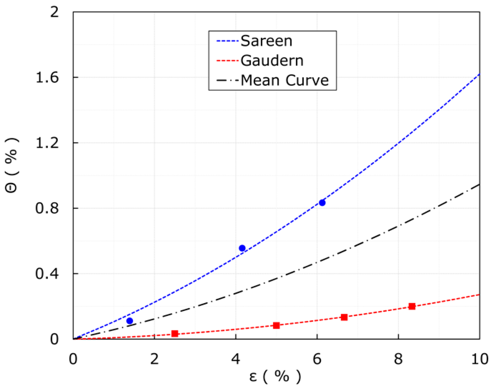
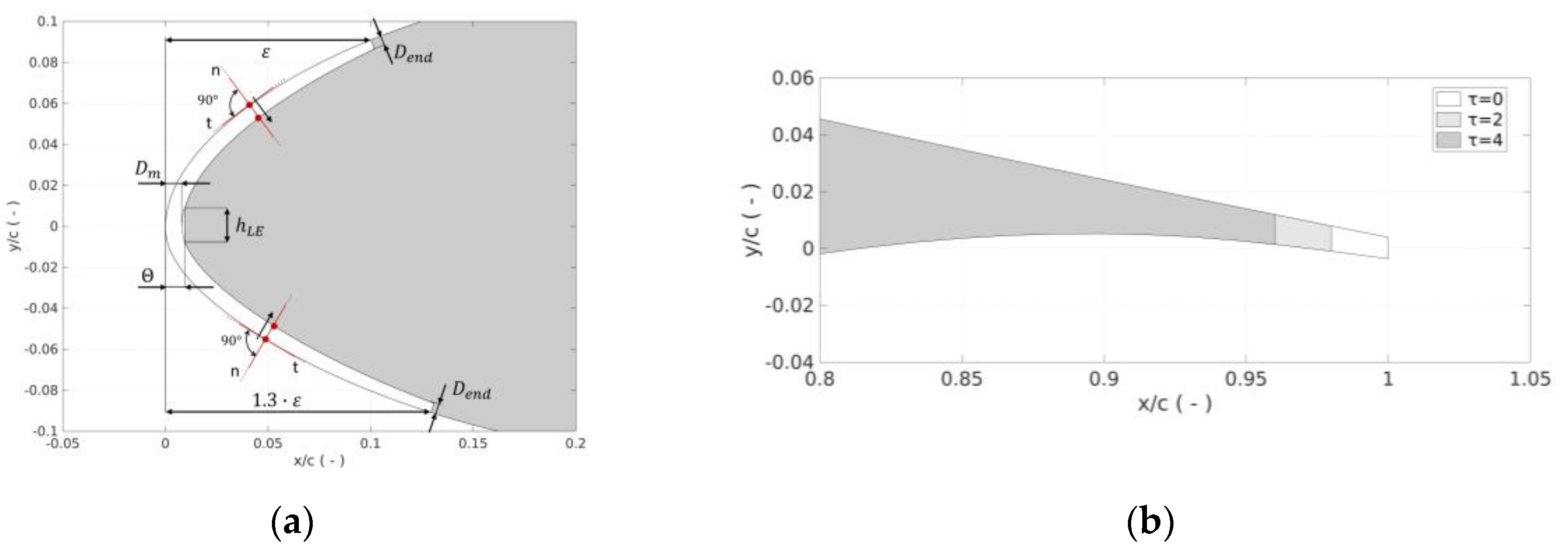
2.3. Blade-Damage Model
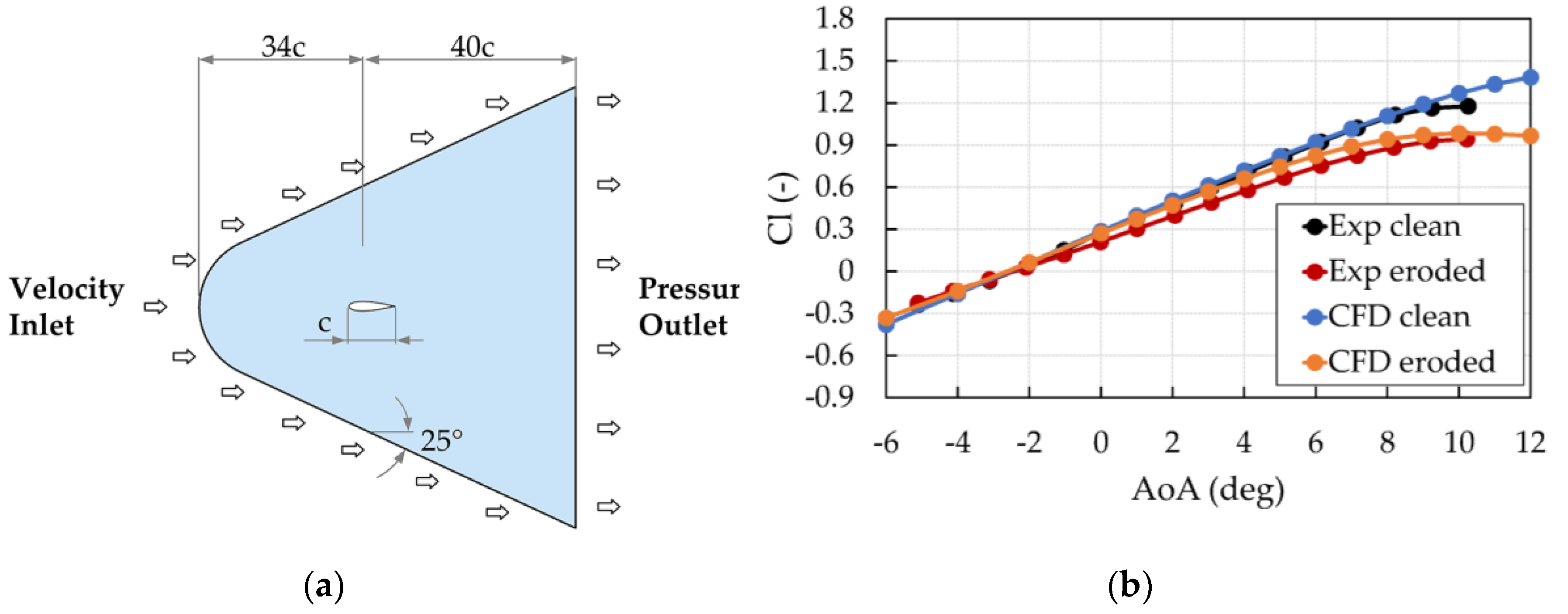
The first stage of the modelling process consists of modelling the blade damage itself. Blade damage is modelled through shape-modification of selected airfoils along the wind turbine’s blades. Trailing-edge damage is reproduced by a simple truncation of the airfoil’s trailing-edge. The amount of TE truncation with respect to the airfoil’s cord is expressed as the above-introduced TE Damage Factor τ. Leading-edge damage is instead modelled through a more complex shape modification. This, which is caused by leading-edge delamination, is based on two main parameters, the maximum erosion depth θ and the chord-wise coverage of the damaged area ε. Both the influence of ε and of θ are studied in this research. However, in order to quickly estimate the global influence of leading-edge damage with respect to trailing-edge damage and to keep the analysis synthetic with only two random input variables, θ and ε were related through an empiric correlation. This assumption is supported by existing studies, where these two variables seem to be related to each other. However, Gaudern et al. [21] and Sareen et al. [5] found two very different ε-θ curves, as shown in Figure 2. As both curves are found by field examination of the blades and given that there is no clear way of assessing which of the two curves is more accurate for this study, a mean curve is proposed here (also shown in Figure 2). We can now refer only to ε as the aforementioned LE Erosion Factor, as this value now also uniquely determines θ.
Once a value of ε is selected, the damaged airfoil shape is generated with a purposely developed Matlab® tool. The LE of the airfoil is moved inward by a maximum depth of θ. Similarly to what was done by Schramm et al. [22], the leading-edge was flattened. The height of the flattened area is imposed to be h = 2 θ . Damage extends up to ε on the suction side of the airfoil and up to 1.3ε on the pressure side, as done in [5]. This is also motivated by the fact that wind turbine airfoils are designed to operate with a positive angle of attack (AoA), and therefore, the pressure side of the airfoil is more exposed to wear. The depth of delamination at the end of the damaged area is equal to D e n d = θ / 3 . The TE and LE damage models are shown in Figure 3. The models are also described in further detail in [10]. The present model is a simplified version of the real LE damage pattern adequate for a parametric study like the present one, which cannot therefore reproduce all the features of a real, three-dimensional damaged blade. The model, however, is in line with the proposals of other authors [22,23] and also qualitatively reproduces the damaged shapes obtained from computational models [8,24], as seen in experiments [5].

2.4. CFD Setup

The lift and drag coefficients of the airfoils are calculated using CFD. The numerical set-up was used by the authors and has been presented in detail in [10]; however, the main parameters will be reassumed herein. The ANSYS® FLUENT® (Version 18.2) solver is used to calculate the 2D polars. A Reynolds-averaged Navier‒Stokes (RANS) approach is used. The Navier‒Stokes equations are solved in a coupled manner with second order upwind spatial discretization. Turbulence closure is achieved with the k-ω Shear Stress Transport (SST) model. A bullet-shaped computational domain is used, as with this shape open-field conditions can be modelled with only one inlet and one outlet boundary condition. In order to ensure that the boundary conditions do not influence the results, the computational domain is 74 chord lengths long and 40 chord lengths wide, as shown in Figure 4a.
An unstructured triangular mesh is used. The airfoil’s boundary layer is modelled with a quadrilateral inflation layer from the blade surface. A total amount of 46 prismatic layers are used. To ensure grid independence, three meshes were tested with varying number of elements. A coarse mesh with 1.3 × 10⁵ elements and 500 elements along the airfoil surface, a medium mesh with 2.8 × 10⁵ elements and 650 elements along the airfoil’s surface, and a fine mesh with 3.6 × 10⁵ elements and 750 elements along the airfoil’s surface. The lift (Cl) and drag (Cd) coefficients are calculated with CFD between 20° and 30° of AoA; values for AoA higher and lower than this are extrapolated using Viterna’s method [25]. A total roughness height of 0.4 mm is imposed on the airfoil’s nose trough an equivalent sand-grain roughness height, estimated through the simple correlations provided in [26]. This roughness height is selected based on the observations of several authors [5,6,21] and models medium to advanced pitting and gauging of the LE. As the focus of the LE damage model is on advanced stages of damage, a constant value of roughness was considered suitable across all the LE-damaged cases.
It is important to point out that CFD is by its nature deterministic, i.e., the same simulation is expected to give the same results if the same settings are used. In this sense, it does not add any source of uncertainty in the analysis. On the other hand, it is true that using different numerical settings to solve the same test case could lead to different results. On this basis, it is very important that the CFD approach is robust and validated with experiments whenever possible. In the present study, in particular, the numerical set-up was validated with respect to available experimental data from [5]. The clean and eroded data is obtained from the DU96W-180 airfoil that was tested in clean and damaged configurations (“stage 5” erosion in [5]) for a Reynolds number of 1.5 × 10⁶. Figure 4b demonstrates good agreement between the experimental values and CFD predictions, with limited differences that can be attributed to the unspecified wind tunnel turbulence level and to the surface finish of the reference model.

2.5. Aeroelastic Setup

The lift and drag coefficients of the damaged airfoils are used in an aero-servo-elastic model of the DTU 10 MW RWT [11]. The model is developed within NREL’s open-source simulation code OpenFAST (NREL, CO, USA) [12]. The aerodynamic module, AeroDyn is based on blade element momentum (BEM) theory. As in all BEM codes, the wake is modelled with a series of concentric annuli, upon which a momentum balance is imposed. The blades are modelled trough lift and drag coefficients. Corrections for high induction (Glauert correction), blade tip and root losses, tower shadow, skewed flow and dynamic stall are included [27]. The coefficients of the dynamic stall model are tuned based on the lift, drag and moment coefficients of the damaged airfoils. Blade damage was considered from 70% of the rotor span outwards. The reasoning behind this choice has to do with the fact that the LE damage phenomena considered are mainly related to erosion, which is most influent where the local blade inflow velocities are highest. Other authors also applied damage from 70% of the rotor span outwards [6]. The lift and drag coefficients of the damaged airfoils are applied uniformly to the entire damaged area.
Fully flexible blades and tower are modelled with the structural dynamics module ElastoDyn. The modal formulation allows for a fairly accurate computation of the structural dynamics with very low computational cost. The Delft Research Controller (DRC) [28] is used in this study. This open-source baseline controller is able to regulate torque and pitch. Constant-torque operation is selected above rated wind speed. The control parameters are tuned based on the report of [29].

2.6. General DLC Setup

The DTU 10 MW RWT is a state-of-the-art reference rotor, developed in recent years as a benchmark for researchers and industry in the field of wind energy. It features a 178-meter diameter rotor with aerodynamic features like gurney flaps that help this conceptual turbine reach a rated power of 10 MW at a wind speed of 11.4 m/s. The tower height is 119 m and the nominal revolution speed is 9.6 rpm, which equates to a tip speed just shy of 90 m/s. The complete definition of the turbine and all of its parameters can be found in Bak et al. [11]. To estimate the AEP of the turbine, a power-production design load case (DLC) is simulated. This is done through sixty-six 10-minute simulations with wind speeds at a hub height between 4 and 24 m/s. Six turbulent seeds per wind speed are simulated, in compliance with the minimum requirements of the IEC 61400-1 [30]. The wind fields also feature wind shear and misaligned flow with respect to the rotor plane. By simulating several cases, uncertainties regarding atmospheric conditions are dealt with, and their influence is accounted for in this study.
It is important to note that turbulence affects power production and other key turbine figures in a complicated manner, as this depends both on the interaction between the controller and the incoming wind speed and on the complex blade boundary-layer phenomena amongst other things. The interaction between large turbines and the turbulent atmospheric boundary layer is out of the interest of the present study and has been evaluated in detail by Churchfield et al. and Nandi et al. [31,32]. Moreover, as other authors have pointed out when studying a similar multi-MW wind turbine in an aero-servo-elastic modelling framework [20], six turbulent realizations are enough to guarantee good convergence on the AEP statistics.
AEP is calculated using a Rayleigh wind-speed probability density function with a mean of 10 m/s as specified by IEC class IA, which is the design class of the DTU 10MW. The AEP obtained using a Rayleigh distribution with a mean wind speed of 8.5 m/s (corresponding to IEC class IIA) will also be briefly analyzed as this could be more representative of the impact of blade damage on sites with lower mean wind speeds.

3. Results

The aPC resulting collocation points are qualitatively shown in Figure 5 and detailed in Table 2. For each point, the corresponding damaged airfoil geometry is generated and CFD calculations were performed as described in Section 2.3. With the resulting airfoil data, aero-servo-elastic BEM simulations were performed as described in Section 2.4.

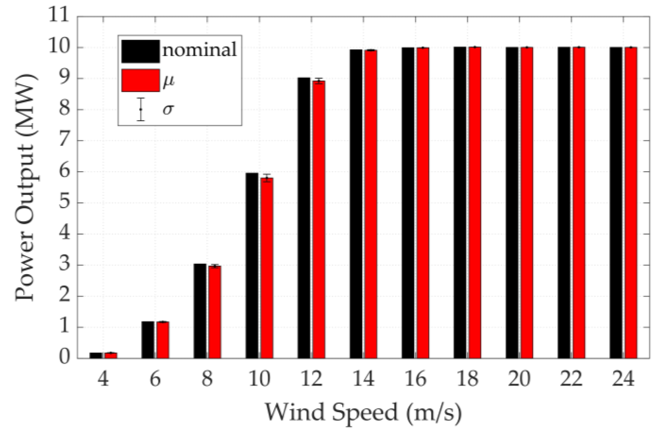
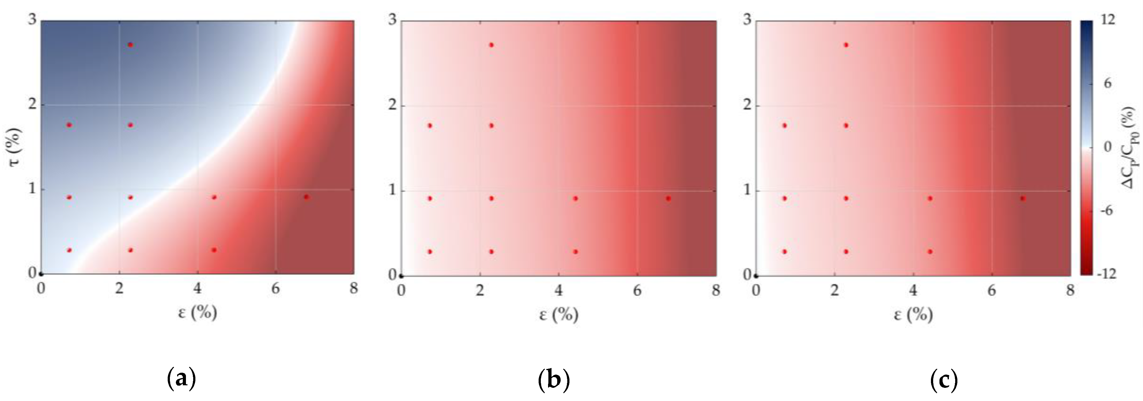
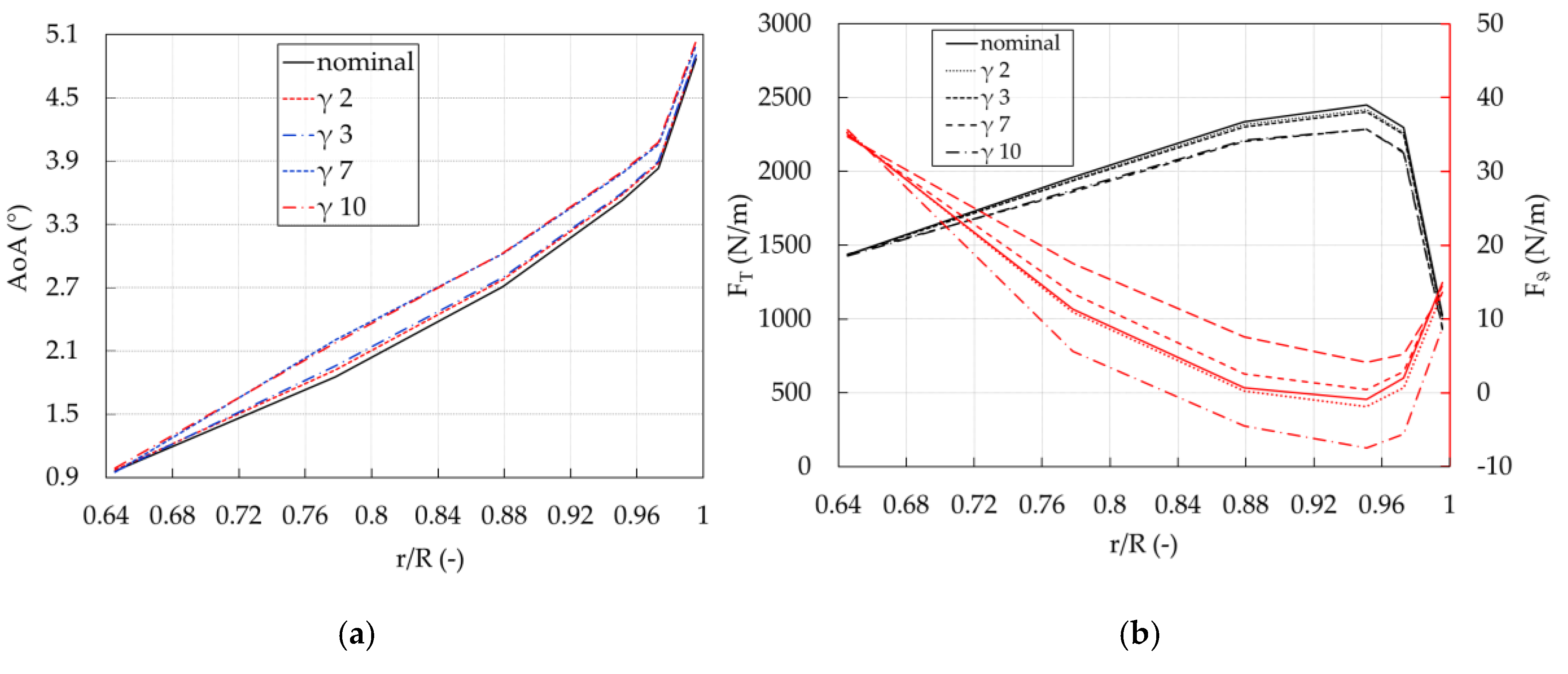
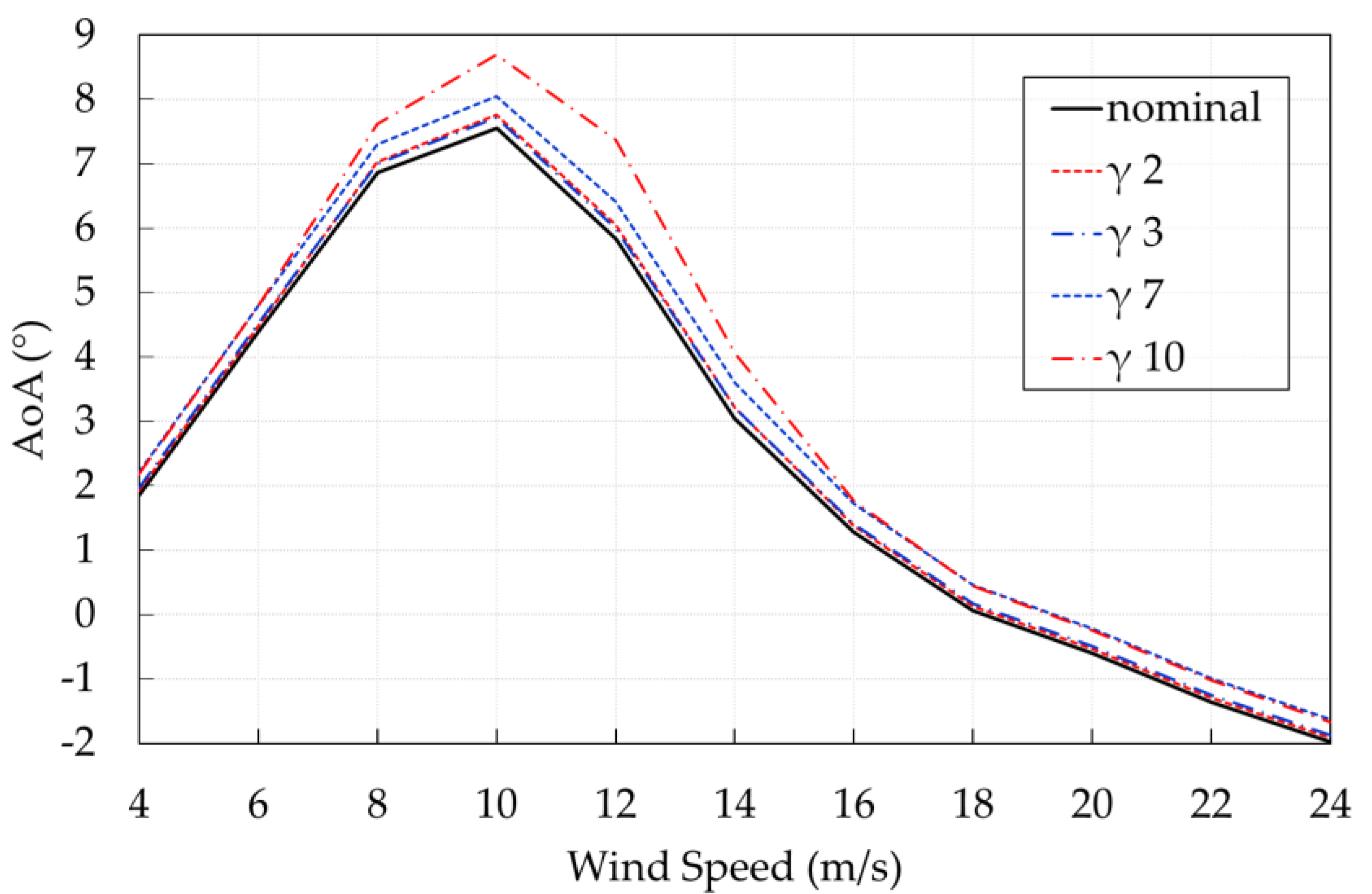
3.1. Aerodynamic Performance

In this section the aerodynamic performance under uncertainties is discussed. In Figure 6 the mean variation in power coefficient (CP) with respect to the clean reference turbine is shown. The standard deviation and associated probability contours are also shown. The CP mean value is lower than the nominal one for all the wind speed bins except for the 4 m/s one. In this wind speed bin, the average gain is about 1%. The reasons that cause such gains are related mainly to the TE damage; however, this gain in performance, while conceptually interesting, is weakened by two factors. First, at 4 m/s the power is about 60 times lower than the nominal one, and thus the effect on the AEP will be minimal. This can be seen clearly in Figure 7. Secondly, there is a high dispersion in the CP values and therefore the expected value is hard to predict. The high dispersion is due to the extremely different response from the damaged airfoils. Both gain and power losses at this wind speed occur. The time averaged AoA from 30% of the blade span to tip goes from 0° to 5°. This allows some of the damaged airfoils to operate with favourable lift and drag forces with respect to others. More details about this behaviour are given below.
The highest value for the mean decrease in CP is of −2.6% at 10 m/s. At this wind speed the reduction in CP can exceed −12%. Moreover, from 8 m/s to 12 m/s, mostly only power losses occur. In this wind speed range, a significant part of the total turbine’s energy is produced; therefore, power reductions in this region will eventually lead to a significant reduction in AEP. Finally, for wind speeds higher than 14 m/s, shown in the grey-shadowed region in Figure 6, the damage effects are no longer visible, as from this wind speed onwards a lower pitch-to-feather regulation is able to compensate for the aerodynamic losses.
The power output per wind speed bin is shown in Figure 7. Upon examination of this figure, it is apparent that the blade damage has a greater impact on power output between 8 m/s and 12 m/s, confirming what was seen in the relative trends of Figure 6. At 4 m/s, however, as previously pointed out, the mean power output is only 174 kW, higher than the 172 kW of the nominal case. Due to the little power produced, this difference as well as the high standard deviation of ±7 kW (±4%) are not visible in the plot, further highlighting how such variation has little impact on the overall performance. In order to better understand the global results, each wind speed bin can be examined more in detail.
The response surfaces reporting the differences in CP for the wind speed bins that show the most relevant differences are shown in Figure 8. For the wind speed bin of 4 m/s the response surface slightly overestimates the CP of the nominal geometry. Such behavior is shown in Figure 8a around the ε = 0, τ = 0 point. On the other hand, the response surface prediction gives good results at 8 m/s and 10 m/s where the CP variation predicted for the nominal geometry is zero as expected.
In the 4 m/s wind speed bin, an increase in CP for several combinations of ε and τ can be noted. To explain this unexpected trend, one can consider the collocation point pairs γ 7 & γ 2 (same ε and the highest and the lowest τ, respectively) and γ10 & γ3 (same τ and the highest and the lowest ε, respectively). Therefore, looking at the pair γ2 & γ7 the influence of τ is highlighted, while looking at the pair γ10 & γ3 the influence of ε is highlighted. Point γ7 shows the highest increase in CP (about 10%), while γ2 shows a mild decrease in CP, about −1.5%; thus, as shown in Figure 8, power increases as tau increases. The other γ-pair shows the opposite behavior, for γ10, the power coefficient decreases by 12%, while γ3 shows an increase in the power coefficient of about 3%, and thus, power decreases as tau decreases. To better understand the trends, the lift and drag coefficients for the FFAW3-241 airfoil (i.e., the airfoil present in the damaged part of the blade) for the four damage levels are shown in Figure 9 with respect to the reference configuration. In general, lift decreases and drag increases for all of the damaged configurations as expected. Focusing on the mean AoA recorded for the various damaged configurations at 4 m/s in Figure 9a, it is clear how the mean AoA increases for all of the damaged cases. This is due to the lower lift of the damaged cases. A new operational equilibrium point in the BEM code is then reached, with a lower induction and thus a higher AoA.
As a consequence of the increased AoA, lift and drag forces slightly increase and, more importantly, are more tangentially and axially oriented. The new force composition generates more torque and more power for some of the combinations of ε and τ. As shown in Figure 10, the same phenomena are occurring for all the damaged configurations: a change in the lift and drag coefficients leads to a different BEM equilibrium point with different induction and AoA along the entire area of the blade affected by damage. However, increasing ε also significantly increases drag, leading to lower performance and offsetting the benefit of a higher AoA, despite the change of orientation of the forces. For instance, in γ10, the highest increases in drag are observed, exceeding 30% at an AoA of around 2°.
In Figure 11 the average AoA for the nominal and four damage combinations for all the wind speed bins is shown. For all the damaged combinations, the highest average AoAs are predicted in the 8 m/s and 10 m/s wind speed bins. At 8 m/s mean wind speed the average AoA for the nominal case at 78% blade span is about 6.9°, while the damaged cases work at an even higher AoA due to decreased induction, as previously discussed. In these wind speed bins, there is no power increase in any combination of ε and τ. From the analysis of Figure 9, the higher the AoA, the wider the difference is in lift and drag coefficients. This ultimately leads to the power losses observed in Figure 6, Figure 7 and Figure 8, with peaks that exceed −10% at 8 m/s and −12% at 10 m/s, respectively. It is also interesting to note that ε is the main cause of performance decrease and has a more pronounced effect than τ. This is due to the fact that LE damage causes a reduction in the stall AoA of the airfoil, which strongly influences high-AoA operation and a more pronounced increase in drag than TE damage.
The probability distributions found from the evaluation of the computed response surfaces at 4 m/s, 8 m/s and 10 m/s are shown in Figure 12. At 4 m/s, the variation in CP is most affected by uncertainties. The peak is located at 1% of variation in CP, but the resulting distribution is fat-tailed. Indeed, the standard deviation is ±4.1% and the probability to lose or gain CP are about 40% and 60%, respectively. At 8 m/s and 10 m/s, the distributions are strongly asymmetric and have lower standard deviations with respect to the 4m/s case and are equal to ±1.7% and ±2% at 8 m/s and 10 m/s, respectively. In both cases, the probability for a CP gain is zero and losses always occur. They both have a marked left tail, but a higher dispersion at 10 m/s is found. The probability peak is clearly located on the right of the mean value at −1.5% and −1.7% for 8 m/s and 10 m/s, respectively.

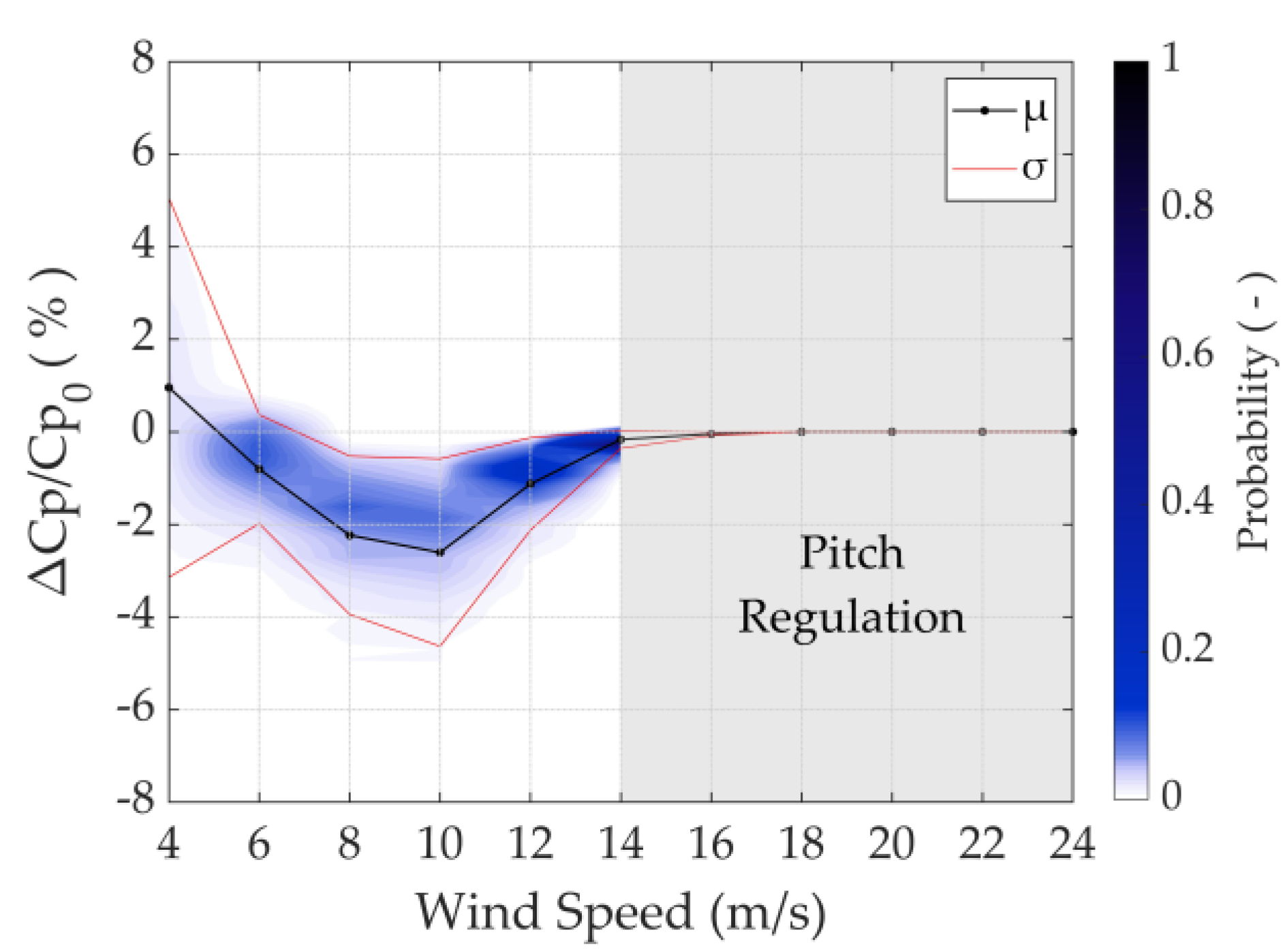
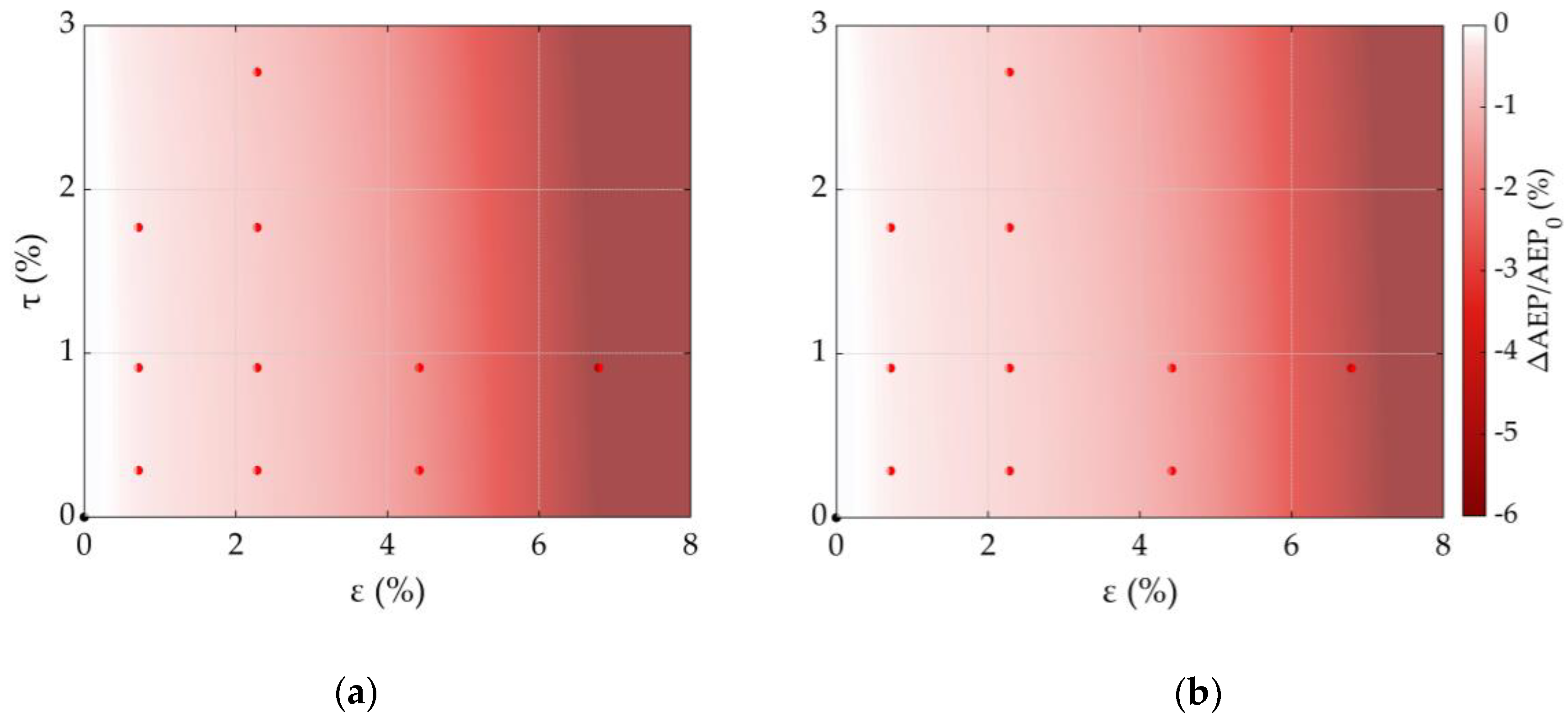
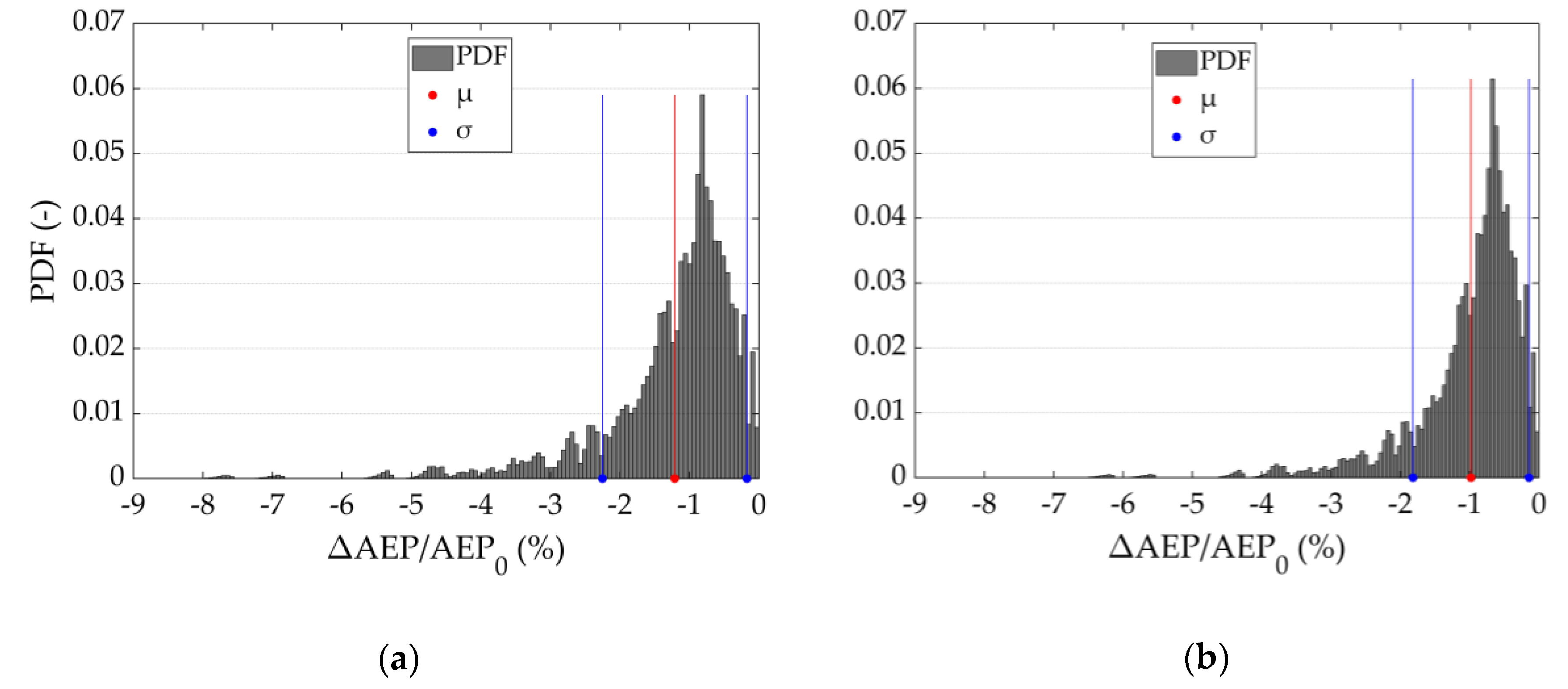
3.2. Annual Energy Production (AEP)

The uncertainties in AEP estimation are discussed in this section. The AEP was calculated according to IEC 61400-1 standard turbine classes. A Weibull wind speed distribution with shape factor of 2 and average values of 8.5 m/s and 10 m/s were used to model sites of IEC wind class II and IA. In particular, class IA is chosen as this is the design class of the DTU 10 MW RWT and class IIA is chosen as representative of medium wind speed sites, where such a turbine might also be installed. The availability factor was assumed to be 1. This assumption is justified by the fact that relative variations are mainly analyzed in the present study. The variation in AEP for the two wind distributions is shown in Figure 13. Both response surfaces well predict the trends around ε = 0, τ = 0, showing no variation in AEP in that point. The LE erosion, ε, is the main driver for AEP reduction, as decreases are mostly along the ε axis. The trailing edge damage, τ, has a minor influence in AEP, as clearly visible in Figure 13. Moreover, the trailing edge damage contribution seems to be dependent on the erosion level. For instance, if one considers the six combinations of ε and τ (where ε = 0, 4, 8 and τ = 0, 3) for wind class IIA shown in Table 3, the point ε = 4, τ = 0 gives a variation in AEP of −1.87%, while the point ε = 4, τ = 3 gives a variation of −2.24%. Therefore, for ε = 4, the trailing edge damage increases losses by 0.37%. By performing the same consideration for ε = 8, trailing edge damage increases losses by 0.82%. This means that the TE contribution to losses increases as ε increases.
The highest variation in AEP predicted by the response surface is −10.35% at ε = 8, τ = 3 for class IIA, as seen in Figure 13a. The highest simulated AEP reduction is −6.21% for γ10 (class IIA, Figure 13a). For wind class IA, the highest variations in AEP are lower than the ones predicted for class IIA and amount to −8.56% in ε = 8, τ = 3 and −5.02 in γ10, as shown in Figure 13b. Such differences are due to the Weibull wind speed PDFs. The probability for the machine to work in the bins range from 8 to 12 m/s, where the highest losses in power occur, are 36% and 31% for IIA and IA, respectively. This difference is the main cause of different variations in AEP for the two classes.
Finally, we consider the probability distributions AEP variation shown in Figure 14. As is also the case for the previously shown distributions, the PDFs are obtained by sampling the response surfaces 250,000 times. The mean and standard deviations of the PDFs are −1.21% and ±1.04% for class IIA and −0.98% and ±0.84% for class IA. Such mean reductions are indeed significant on a multi-MW scale turbine and are in line with the finding of Eisenberg et al. [33] but seem to be lower than the values indicated by most of the present research [5,6,8]. Both distributions show a clear peak, with the mode of the PDFs below 1% AEP loss in both cases. For both the IEC 61400-1 IA and IIA scenarios, the left tails of the distributions are long, reaching values of 6–8% AEP reductions, coherently with the response surface shown in Figure 13. The probability associated to values of AEP reduction in the order of 3–8%, which most authors indicate, is almost insignificant in the present test case. It is important to stress that these results depend on the assumed PDFs, which are, as discussed, based on published literature and appear reasonable based on the authors’ experience. Moreover, as Fiore and Selig have suggested [34], larger turbines seem to be impacted less by LE damage phenomena such as erosion. However, results suggest that the commonly forecasted reductions might be based on heavy-damage scenarios, which, whilst not unrealistic, have low probability of occurrence.
The wind class IIA shows higher standard deviation and higher left tail length. As previously mentioned, which is due to the fact that in the class IIA scenario the turbine operates at rated power for a shorter period of time with respect to the class IA scenario. In fact, as also pointed out by Eisenberg [33], the turbine’s power output does not experience any significant variation for wind speeds above rated when the blades are damaged and therefore the higher the mean wind speed, the lower the variation in AEP. These results clearly depend on the IEC class that was chosen. Lowering the average wind speeds even further (IEC Class III), the turbine is expected to spend less time at rated power, and therefore, AEP losses are expected to further decrease for the present test case. Although low wind speed sites have recently been exploited for wind turbine installation, specially designed machines with low specific power are being installed in such sites, resulting in machines that are able to spend significant time at rated power even in these sites. As noted in [33], a utility-scale machine will spend 40% to 60% of its time at rated power, where blade damage has no effects. In addition, although the main cause of LE erosion is related to the rotational tip velocity, it can be argued that in lower wind speed sites, less transport of abrasive particles will arise, therefore leading to less erosion.

4. Conclusions

This study proposes the use of an uncertainty quantification approach to the modelling of the effects of blade damage on the performance of multi-MW wind turbines. The proposed approach aims at overcoming some of the issues associated with the evaluation of a single test case. In fact, treating blade damage as a random phenomenon, bias due to a specific test case of a combination of blade-damaging factors can be avoided and more general conclusions can be drawn. The entire process is simulated numerically. First, geometric shape modifications are applied to the airfoils that constitute the turbine’s blade. Lift and drag coefficients are calculated using CFD. The newly found coefficients are then applied to an aero-servo-elastic model of the wind turbine. Uncertainties are propagated through the model using an arbitrary polynomial chaos method.
Results show that LE damage has the larger influence on power and AEP losses. For the selected test case, TE damage has little impact, except for when the turbine is operating at very low wind speeds, where a slight performance increase is observed due to TE damage. Focusing on absolute values, maximum average power reductions are observed at 8 m/s and 10 m/s mean wind speeds and are of 2.2% and 2.6%, respectively. The most unfavorable damage combinations simulated showed a decrease in AEP of up to over 6%. By looking at the probabilistic framework, however, the configurations with the highest probability of occurring based on the input PDFs show AEP reductions of below 1% in both IEC classes I and IIA. Indeed, mean AEP reductions of just below 1% for class IA and just above 1% for class IIA are estimated. These values, whilst significant, seem to be notably lower than what is commonly forecasted in published literature that, however, is strictly site- or turbine-dependent. It is important to point out that the results of the present study do not indicate that published literature values are unrealistic (even though sometimes a too large span coverage of erosion is considered), however, for the present test case, representative of modern turbine size and design trends, such values seem to have very low probabilities of occurrence. Indeed, AEP decreases exceeding 10% are noted in the present study. Blade damage is an issue that should still be taken very seriously by the industry, due to its structural implications that were not investigated in the present work; however, the impact on AEP does not seem to be as pronounced as early research indicated. A great deal of factors could cause these discrepancies, which could be due to the radial damage extension considered and size and hence the Reynolds number of the turbine, which are not investigated herein and therefore remain an open issue, where additional research would definitely be beneficial. As pointed out by other authors, LE damage seems to have a lower effect on larger wind turbines. Although this is not the focus of the present work, the results of this study, if put into perspective with other published literature that reports higher AEP decreases on smaller turbines, seem to confirm this.
Moreover, as previously discussed, the results strongly depend on the input PDFs. The presented method can be however adapted to different input PDFs, which are hopefully more extensively supported by field data. Nevertheless, the present assumptions can be considered realistic for medium-low damaging environments or for blades where regular maintenance schedules are planned. It is also important to point out that these results are valid strictly only for the present test case. A selection of different study cases might influence the results significantly, as, in the authors’ experience, LE damage affects different airfoils to different degrees. Finally, the LE damage model also influences the results. Although the model is calibrated and tested with respect to experimental data and is adequate for the present parametric framework, it is hard, if not impossible, to accurately reproduce small, stochastic features that might influence the sectional efficiency significantly.
In conclusion, even considering these factors, it is apparent that the present statistical approach is able to give designers a better picture of the impact of blade damage.

Author Contributions

Conceptualization, F.P. and A.B.; methodology, F.P., L.C., S.S.; software, F.P., L.C., M.C.; formal analysis, A.B., F.P.; investigation, F.P., L.C.; resources, A.B.; data curation, F.P., L.C., A.B.; writing—original draft preparation, F.P., L.C.; writing—review and editing, A.B., S.S.; visualization, F.P.; supervision, S.S., M.C., A.B.; project administration, A.B. All authors have read and agreed to the published version of the manuscript.

Funding

This research received no external funding.

Conflicts of Interest

The authors declare no conflicts of interest.

Nomenclature

Acronyms
AEPAnnual energy production, kWh
aPCArbitrary polynomial chaos
BEMBlade element momentum
CFDComputational fluid dynamics
DLCDesign load case
DRCDelft research controller
IECInternational electrotechnical commission
LELeading edge
PCPolynomial chaos
PCM Probabilistic collocation point
PDFProbability desity function
RANSReynolds averaged navier stokes
SST Shear stress transport
TETrailing edge
Latin Letters
AoAAngle of attack, deg.
cBlade chord, m
ciExpansion coefficients
CdDrag coefficient
ClLift coefficient
CPTurbine power coefficient
DendDelamination depth at the end of damaged area, m
FTThrust force, N/m
FϑTangential force, N/m
hLeading edge flattened area height, m
P(i)Orthogonal polynomials
RMPolinomial expansion remainder
YSpecific output of interest
Greek Letters
α, βBeta function’s shape parameters
γCollocation point
εLeading edge erosion factor
ΘLeading edge erosion depth
μMomentum
ξGeneric aleatory variable
σStandard deviation
τTrailing edge damage factor
ωWeighting term

References

  1. Rempel, L. Rotor Blade Leading Edge Erosion-Real Life Experiences. Wind Syst. Mag. 2012, 11, 22–24. [Google Scholar]
  2. Røndgaard, F.-K. February 23, Ersen-; Europe, 2018 Structural Failure Denmark UK WindAction|Siemens Sets Billions: Ørsted must Repair Hundreds of Turbines. Available online: http://www.windaction.org/posts/47883-siemens-sets-billions-orsted-must-repair-hundreds-of-turbines#.XfzepkdKiUl (accessed on 20 December 2019).
  3. Régis, D. Why Inspect Wind Turbine Blades? How to Avoind Major Wind Turbine Blade Damage and Cost. Sustainable Energy Consulting and Software (3E). 2014. Available online: https://www.3e.eu/wp-content/uploads/2014/06/3E_Why-Wind-Turbine-Blade-Inspections_20140507_final.pdf (accessed on 10 July 2020).
  4. Wood, K. Blade Repair: Closing the Maintenance Gap. Available online: https://www.compositesworld.com/articles/blade-repair-closing-the-maintenance-gap (accessed on 9 June 2020).
  5. Sareen, A.; Sapre, C.A.; Selig, M.S. Effects of leading edge erosion on wind turbine blade performance: Effects of leading edge erosion. Wind Energ. 2014, 17, 1531–1542. [Google Scholar] [CrossRef]
  6. Han, W.; Kim, J.; Kim, B. Effects of contamination and erosion at the leading edge of blade tip airfoils on the annual energy production of wind turbines. Renew. Energy 2018, 115, 817–823. [Google Scholar] [CrossRef]
  7. Jonkman, J.; Butterfield, S.; Musial, W.; Scott, G. Definition of a 5-MW Reference Wind Turbine for Offshore System Development; Technical Report NREL/TP-500-38060, 947422; National Renewable Energy Laboratory: Golden, CO, USA, 2009.
  8. Castorrini, A.; Corsini, A.; Rispoli, F.; Venturini, P.; Takizawa, K.; Tezduyar, T.E. Computational analysis of performance deterioration of a wind turbine blade strip subjected to environmental erosion. Comput Mech. 2019, 64, 1133–1153. [Google Scholar] [CrossRef]
  9. Herring, R.; Dyer, K.; Martin, F.; Ward, C. The increasing importance of leading edge erosion and a review of existing protection solutions. Renew. Sustain. Energy Rev. 2019, 115, 109382. [Google Scholar] [CrossRef]
  10. Papi, F.; Cappugi, L.; Bianchini, A.; Perez-Becker, S. Numerical Modeling of the Effects of Leading-Edge Erosion and Trailing-Edge Damage on Wind Turbine Loads and Performance; ASME TurboExpo: London, UK, 2020. [Google Scholar]
  11. Bak, C.; Zahle, F.; Bitsche, R.; Kim, T.; Yde, A.; Henriksen, L.C.; Natarajan, A.; Hansen, M. Description of the DTU 10 MW Reference Wind Turbine; DTU Wind Energy: Copenhagen, Denmark, 2013. [Google Scholar]
  12. OpenFAST. Available online: https://github.com/OpenFAST (accessed on 31 October 2019).
  13. Oladyshkin, S.; Nowak, W. Data-driven uncertainty quantification using the arbitrary polynomial chaos expansion. Reliab. Eng. Syst. Saf. 2012, 106, 179–190. [Google Scholar] [CrossRef]
  14. Iaccarino, G. Quantification of Uncertainty in Flow Simulations Using Probabilistic Methods; VKI Lecturers Series; von Karman Institute: Rhode-St-Genèse, Belgium, 2009. [Google Scholar]
  15. Carnevale, M.; Montomoli, F.; D’Ammaro, A.; Salvadori, S.; Martelli, F. Uncertainty Quantification: A Stochastic Method for Heat Transfer Prediction Using LES. J. Turbomach 2013, 135, 1–8. [Google Scholar] [CrossRef]
  16. Ahlfeld, R.; Montomoli, F.; Carnevale, M.; Salvadori, S. Autonomous Uncertainty Quantification for Discontinuous Models Using Multivariate Padé Approximations. J. Turbomach 2018, 140. [Google Scholar] [CrossRef]
  17. Tatang, M.A.; Pan, W.; Prinn, R.G.; McRae, G.J. An efficient method for parametric uncertainty analysis of numerical geophysical models. J. Geophys. Res. Atmos. 1997, 102, 21925–21932. [Google Scholar] [CrossRef]
  18. Carnevale, M.; D’Ammaro, A.; Montomoli, F.; Salvadori, S. Film Cooling and Shock Interaction: An Uncertainty Quantification Analysis with Transonic Flows; American Society of Mechanical Engineers Digital Collection: New York, NY, USA, 2014. [Google Scholar]
  19. Salvadori, S.; Carnevale, M.; Fanciulli, A.; Montomoli, F. Uncertainty Quantification of Non-Dimensional Parameters for a Film Cooling Configuration in Supersonic Conditions. Fluids 2019, 4, 155. [Google Scholar] [CrossRef] [Green Version]
  20. Bortolotti, P.; Canet, H.; Bottasso, C.L.; Loganathan, J. Performance of non-intrusive uncertainty quantification in the aeroservoelastic simulation of wind turbines. Wind Energy Sci. 2019, 4, 397–406. [Google Scholar] [CrossRef] [Green Version]
  21. Gaudern, N. A practical study of the aerodynamic impact of wind turbine blade leading edge erosion. J. Phys. Conf. Ser. 2014, 524, 012031. [Google Scholar] [CrossRef]
  22. Schramm, M.; Rahimi, H.; Stoevesandt, B.; Tangager, K. The Influence of Eroded Blades on Wind Turbine Performance Using Numerical Simulations. Energies 2017, 10, 1420. [Google Scholar] [CrossRef] [Green Version]
  23. Cavazzini, A.; Minisci, E.; Campobasso, M.S. Machine Learning-Aided Assessment of Wind Turbine Energy Losses due to Blade Leading Edge Damage.; American Society of Mechanical Engineers Digital Collection: New York, NY, USA, 2019; IOWTC2019-7578. [Google Scholar]
  24. Fiore, G.; Selig, M.S. Simulation of Damage Progression on Wind Turbine Blades Subject to Particle Erosion. In Proceedings of the 54th AIAA Aerospace Sciences Meeting; American Institute of Aeronautics and Astronautics, San Diego, CA, USA, 4–8 January 2016. [Google Scholar]
  25. Viterna, L.A.; Janetzke, D.C. Theoretical and Experimental Power from Large Horizontal-Axis Wind Turbines; National Aeronautics and Space Administration: Cleveland, OH, USA, 1982.
  26. Adams, T.; Grant, C.; Watson, H. A Simple Algorithm to Relate Measured Surface Roughness to Equivalent Sand-grain Roughness. IJMEM 2012, 1, 66–71. [Google Scholar] [CrossRef]
  27. Wind Energy: Handbook; Burton, T. (Ed.) J. Wiley: Chichester, UK; New York, NY, USA, 2001; ISBN 978-0-471-48997-9. [Google Scholar]
  28. Mulders, S.; van Wingerden, J. Delft Research Controller: An open-source and community-driven wind turbine baseline controller. J. Phys. Conf. Ser. 2018, 1037, 032009. [Google Scholar] [CrossRef] [Green Version]
  29. Borg, M. LIFES50+ Deliverable D1.2: Wind Turbine Models for the Design; DTU Wind Energy: Risø, Denmark, 2015; p. 29. [Google Scholar]
  30. International Electrotechnical Commission. Wind Turbines-Part1: Design Requirements; Technical Standard IEC61400-1:2005; International Electrotechnical Commission: Geneva, Switzerland, 2005. [Google Scholar]
  31. Churchfield, M.J.; Lee, S.; Michalakes, J.; Moriarty, P.J. A numerical study of the effects of atmospheric and wake turbulence on wind turbine dynamics. J. Turbul. 2012, 13, N14. [Google Scholar] [CrossRef]
  32. Nandi, T.N.; Herrig, A.; Brasseur, J.G. Non-steady wind turbine response to daytime atmospheric turbulence. Phil. Trans. R. Soc. A 2017, 375, 20160103. [Google Scholar] [CrossRef] [PubMed]
  33. Eisenberg, D.; Laustsen, S.; Stege, J. Wind turbine blade coating leading edge rain erosion model: Development and validation. Wind Energy 2018, 21, 942–951. [Google Scholar] [CrossRef]
  34. Fiore, G.; Selig, M.S. Simulation of Damage for Wind Turbine Blades Due to Airborne Particles. Wind Eng. 2015, 39, 399–418. [Google Scholar] [CrossRef]
Figure 1. Flowchart of the uncertainty-quantification procedure.
Energies 13 03785 g001
Figure 2. ε-θ correlation in literature [5,21] and proposed correlation in black point-dashed line.
Energies 13 03785 g002
Figure 3. Damage modeling. (a) Leading-edge (LE) damage; (b) TE damage.
Energies 13 03785 g003
Figure 4. CFD validation: (a) Illustration of the adopted computational domain; (b)validation of the numerical setup in respect to data from [5] at Re = 1.5 × 10⁶.
Energies 13 03785 g004
Figure 5. Arbitrary polynomial chaos (aPC) resulting collocation points’ plot in ε–τ space.
Energies 13 03785 g005
Figure 6. Variation in power coefficient, mean value (μ), standard deviation (σ) and probability.
Energies 13 03785 g006
Figure 7. Power output per wind speed bin for nominal and mean damaged (μ) turbine with standard deviation (σ).
Energies 13 03785 g007
Figure 8. Variation in power coefficient. Response surfaces as contour plots at (a) 4 m/s, (b) 8 m/s and (c) 10 m/s.
Energies 13 03785 g008
Figure 9. Aerodynamic coefficients for nominal and most significant power coefficients (CPs): (a) Lift coefficient; (b) drag coefficient.
Energies 13 03785 g009
Figure 10. Relevant turbine figures: (a) Angle of attack along the outer part of the blade and (b) thrust (FT) and tangential (Fϑ) for the outer part of the blade at 4 m/s mean wind speed.
Energies 13 03785 g010
Figure 11. Angle of attack vs. wind speed for nominal and four damaged conditions at 78% blade span.
Energies 13 03785 g011
Figure 12. Variation in power coefficient probability density functions (PDFs) with mean value (μ) and standard deviation (σ) at (a) 4 m/s, (b), 8 m/s and (c) 10 m/s.
Energies 13 03785 g012
Figure 13. Variation in AEP. Response surfaces as contours plot for wind classes (a) IIA and (b) IA.
Energies 13 03785 g013
Figure 14. Variation in AEP PDFs for wind classes (a) IIA and (b) IA.
Energies 13 03785 g014
Table 1. Probability density functions for erosion factor andTrailing Edge (TE) damage factor.
ParameterPDFαβSupport
εBeta2.06.00–10 (%)
τBeta2.06.00–4 (%)
Table 2. aPC optimal collocation points values.
γ12345678910
ε2.27922.27920.71342.27920.71344.41892.27920.71344.41896.7884
τ0.91180.28540.91181.76770.28540.91182.71571.76770.28540.9118
Table 3. Annual Energy Production (AEP) reduction for some of the computed ε-τ combinations.
ετΔAEP/AEP0 (%)
000.00
030.00
40−1.87
43−2.24
80−9.69
83−10.51

