Capacity Planning of Distributed Wind Power Based on a Variable-Structure Copula Involving Energy Storage Systems

Abstract

Distributed wind power (DWP) needs to be consumed locally under a 110 kV network without reverse power flow in China. To maximize the use of DWP, this paper proposes a novel method for capacity planning of DWP with participation of the energy storage system (ESS) in multiple scenarios by means of a variable-structure copula and optimization theory. First, wind power and local load are predicted at the planning stage by an autoregressive moving average (ARMA) model, then, variable-structure copula models are established based on different time segment strategies to depict the correlation of DWP and load, and the joint typical scenarios of DWP and load are generated by clustering, and a capacity planning model of DWP is proposed considering investment and operation cost, and environmental benefit and line loss cost under typical scenario conditions. Moreover, a collaborative capacity planning model for DWP and ESS is prospectively proposed. Based on the modified IEEE-33 bus system, the results of the case study show that the DWP capacity result is more reasonable after considering the correlation of wind and load by using a variable-structure copula. With consideration of the collaborative planning of DWP and load, the consumption of DWP is further improved, the annual cost of the system is more economical, and the quality of voltage is effectively improved. The study results validate the proposed method and provide effective reference for the planning strategy of DWP.

1. Introduction

There are generally two typical integration forms of wind power into power systems: centralized and distributed. Distributed wind farms do not transport wind power over large-scale long-distance transmission lines, they are directly provided to the load center of the power system [1,2], and the generated electricity is consumed locally. Distributed wind power (DWP) has become an effective solution for improving China’s environmental issues, and it will be an important form of wind power integration into the power grid.

For the development and construction of DWP projects, China’s 2018 document [3] presented that the DWP needs to be locally consumed through a 110 kV network with no power delivery at higher voltage levels, and the installed DWP capacity limit should be based on the lowest consumption of load. There is no doubt that this capacity planning principle for DWP will reduce the use rate of wind power greatly, lead to waste of wind resources, and decrease the revenue of wind power industries, further hindering the development of DWP.

At present, many effective models and algorithms for wind power planning in distribution networks have been explored [4,5,6]. A multi-objective DWP planning model was proposed in [7] to meet the operation of unbalanced distribution systems, and the decision framework provided in [8] could optimize DWP planning through technology selection. These studies provide a good reference for further development of wind power in the distribution system.

To comply with the regulations under the premise of local consumption in the distribution system without reverse power flow, it is necessary to further investigate the correlation between DWP and load. At present, Nataf inverse transformation [9,10] and the correlation coefficient matrix method [11] are usually employed for multivariable correlation analysis. However, the correlation feature or correlation matrix between random variables must be determined in advance. When the correlation between variables is complex or the features are not obvious, the fitting effect with the above commonly used models is usually not good. In addition, it is also necessary to take into consideration different scenarios of DWP and load because of their stochastic characteristics [12,13,14]. In [15], the correlation among historical wind, photovoltaic power and electricity demand and the random moments is captured by generating a scenario matrix, but the variable structure is not sufficiently considered. In view of the above issues, copula theory [16] is employed in this work to better describe the correlation between DWP and load, and at different time segments, a variable-structure copula model is established to construct the correlation between DWP and load.

To follow the principle of no reverse power flow to higher voltage level and make the best consumption of renewable resources, one effective way is to bring in the energy storage system (ESS) at the planning stage [17,18,19]. A joint optimization in [17] was proposed to plan the capacity and location of ESS, and distributed generating units in a stand-alone micro-grid were presented. These studies mainly implement collaborative planning from the perspective of economics and pricing-based demand response [20], thus providing a good reference for this paper. Still, the consideration of construction investment, system line loss cost and the maintenance cost of ESS as part of the model’s objective requires further improvement. Based on the above research, this paper takes the network line loss, the investment operation cost and environmental income, and the time-of-day tariff into the objective functions of the planning strategy, and prospectively proposes a feasible collaborative capacity planning model of DWP and ESS. This paper contributes as follows:

(1) To describe the tail correlation and the change of correlation between DWP and load, a variable- structure copula model is employed. In this paper, the variable-structure copula models are constructed using two different time division methods (monthly and quarterly), and strategies are evaluated by constructing an empirical copula model.

(2) Based on the correlation model of the variable-structure copula, the typical scenarios containing correlation information are obtained through the clustering method, and then the DWP capacity planning model is constructed under the typical scenarios. Furthermore, in order to increase the consumption of DWP, a collaborative planning model is established for wind storage, and the consumption of wind power and the quality of voltage level are analyzed based on a typical schedule day.

The structure of this paper is as follows. In Section 2, the autoregressive moving average model (ARMA) model for data prediction of DWP and load is introduced, the correlation of DWP and load based on the variable-structure copula is investigated, and joint typical scenarios are generated using the clustering method. In Section 3, a novel capacity planning model of DWP is proposed under typical scenarios, and a collaborative capacity planning model is further established for DWP and ESS to increase the consumption of wind power. A case study is then carried out in Section 4 based on practical data for wind farm and load. Section 5 summarizes the findings.

2. Correlation Analysis between DWP and Load Based on a Variable-Structure Copula

The wind power output of a distributed wind farm should be consumed by its local load. Since DWP has the characteristics of intermittency and inverse peak shaving, the correlation between DWP and load consumption should be carefully investigated. In this section, a variable-structure copula model is employed to describe the joint density of DWP and local load. This method can well capture the nonlinear, asymmetry and tail correlation characteristics among variables, it can analyze the marginal distribution of each random variable individually, and can also illustrate the varied correlated structure between variables.

2.1. Data Preparation Based on an ARMA Model

To carry out the correlation study between DWP and load, the predicted data of DWP and local load in the planning stage are first obtained by ARMA model. The ARMA short-term prediction model includes the autoregressive part and the moving average part, and its formula is:

$$Y_t={\displaystyle \sum _{i=1}^q{\alpha }_i}{\epsilon }_{t-i}+{\displaystyle \sum _{i=1}^p{\beta }_i}{Y}_{t-i}+{\epsilon }_t,$$

(1)

where Y_t is the value of DWP or load at point t of series; ε_t and ε_t−i are the prediction error term at t and i time points ahead of t, respectively; α is the correlation coefficient, which reflects the dependence of the prediction error at different segments; Y_t−i is the value with i time points ahead of t; β is the correlation coefficient; p is the order of autoregressive process; and q is the order of moving average process.

The order of the ARMA model can be determined by calculating the Akaike Information Criterion (AIC) value of the ARMA with different (p, q) pairs. The optimal ARMA (p, q) model is selected when the AIC value is the smallest.

For cases where there is no historical data of DWP in the local area, the centralized wind power data near the area can be used as a reference, since they have a similar wind source, and the data can be converted proportionally into the DWP capacity for prediction and planning analysis.

2.2. Theory of Copula Function

Based on the predicted time series of DWP and load at the planning stage, in this subsection, this paper proposes a variable-structure copula to depict the correlation between DWP and load.

2.2.1. The Definition and Properties of the Copula Function

Because DWP and load have the characteristics of fluctuation, and DWP also has the characteristic of inverse peak shaving, the correlation between wind power and load is very complicated, and correlation under extreme conditions (tail correlation) cannot be ignored. Therefore, the copula is a useful tool for characterizing nonlinear correlation and tail correlation [21,22] between DWP and load.

Copula theory states that there must exist a copula function that satisfies $F(x,y)=C(F_1(x),F_2(y))$ [23], where $F(\cdot )$ is a 2-dimensional cumulative distribution function, $C(\cdot )$ is a distribution function of two-element copula function, x and y are the samples of DWP and load (MW), respectively, and $F_1(\cdot )$, $F_2(\cdot )$ are the marginal probability density functions of DWP and load, respectively. To simplify, let u = F₁(x), v = F₂(y), and vector u_i and v_i are the values of F₁(x) and F₂(y) at point i.

As a result, to construct a copula model, the first step is to estimate the marginal distribution of DWP and load. Next, a copula function should be carefully selected to fit the correlation between marginal distributions based on some evaluation indices.

2.2.2. Evaluation Indices of Copula Function

After estimating the marginal distribution function of DWP and load, respectively, this paper estimates the parameters based on maximum likelihood estimation (MLE), and the evaluation indices can subsequently be calculated.

The parameter estimation results of Gaussian copula and t copula are the same as Pearson coefficient, which can reflect variables’ linear correlation

$${\rho }_p=\frac{{\displaystyle {\sum }_{i=1}^n\left(u_i-\overline{u}\right)}\left(v_i-\overline{v}\right)}{\sqrt{{{\displaystyle {\sum }_{i=1}^n\left(u_i-\overline{u}\right)}}^2}\sqrt{{{\displaystyle {\sum }_{i=1}^n\left(v_i-\overline{v}\right)}}^2}},$$

(2)

where $\overline{u}$ and $\overline{v}$ are the expected values of the vectors u_i and v_i, respectively, and ${\rho }_p$ is the Pearson coefficient of the vector u_i and v_i.

The evaluation indices also include Kendall coefficient, Spearman coefficient and Euclidean index [24].

(1) Kendall coefficient ρ_k can reflect the nonlinear correlation of the change trend of the vectors u_i and v_i

$${\rho }_k=\frac{4r}{n(n-1)}-1,$$

(3)

where r is the number of the vectors u_i and v_i, whose two attribute values have the same size relationship.

(2) Spearman coefficient ρ_z can reflect the correlation of the rank of the variables

$${\rho }_Z=1-\frac{6{\displaystyle \sum d_i^2}}{n(n^2-1)},$$

(4)

where d_i is the rank differences between two vectors u_i and v_i.

(3) Euclidean index can reflect the distance between the model and the empirical copula model [25].

$$d_x^2={\displaystyle \sum _{i=1}^n{\left|C_m(u_i,v_i)-C_x(u_i,v_i)\right|}^2},$$

(5)

where C_m(u_i,v_i) is the empirical copula function of DWP and load, and C_x(u_i,v_i) is the basic copula functions, where the smaller the Euclidean distance is, the more accurate the model is.

Copula functions used in this paper include Gaussian copula, t copula, Frank copula, Gumbel copula and Clayton copula. To carry out the model evaluation of copula functions, the evaluation indices should be calculated and compared with the empirical copula, as shown in (6) [25].

$$C_m(u_i,v_i)=\frac{1}{n}{\displaystyle \sum _{i=1}^n{I}_{(F_m(x_i)\le u_i)}}{I}_{(G_m(y_i)\le v_i)},$$

(6)

where F_m(x_i) and G_m(y_i) are the empirical distribution functions of DWP and load, respectively, $I(\cdot )$ represents explanatory function, and u and v follow 0-1 distribution satisfying $F(x_i)\le u_i$, $I_{(F(x_i)\le u_i)}=1$.

2.2.3. Variable-Structure Copula

According to the stochastic characteristic of DWP and load, their joint distribution can exhibit varied correlation features at different periods; under these conditions, a unique copula function cannot sufficiently describe the change. The variable-structure copula provides the most suitable copula model for the description of correlation at different stages according to the varied structural features of DWP and load, and is able to capture the changes of related structures between them more flexibly [26].

In general, the variable-structure copula can be divided into three types [27,28]:

(1)

Only the marginal distribution of a single variable has a variable structure;

(2)

The copula function part with a definite marginal distribution possesses a variable structure;

(3)

Both the marginal distribution of a single variable and the copula function possess variable structures.

In this work, both the marginal distribution of a single variable and the joint copula function are modeled with variable structures. Based on different time division strategies, the main steps of constructing the variable-structure copula model are as follows:

(1)

Divide the time series of DWP and load into multiple time segments;

(2)

Apply non-parametric estimation to determine the marginal distribution of each variable at each time segment;

(3)

Construct the copula model at each time segment;

(4)

Perform parameter estimation, evaluate the candidate models and select the optimal copula for each time segment;

(5)

Compare the results based on different time division methods based on (6), and choose the most appropriate division strategy.

For each phased copula function, a binary frequency histogram between variables can be used intuitively as a first estimate of the joint density function selection of DWP and load. By means of the MLE method, the parameters of each basic copula model can be calculated [29]. Based on the evaluation indices of candidate copulas and empirical copula, the two-stage filtration method [30] is used to choose the optimal copula model.

After the modeling of the variable-structure copula, typical scenarios can be generated for further DWP planning.

2.3. Typical Scenario Generation

Based on the continuous variable-structure copula function, it is necessary to discretize it to obtain discrete DWP and load data pairs, so as to provide typical scenarios for the capacity planning of a distributed wind farm.

This paper uses K-means clustering to classify typical scenarios. The specific steps are as follows:

(1)

Discretize each phased copula function to generate two-dimensional discrete data pairs.

(2)

Set the number of typical scenarios and select the initial condensation point.

(3)

Calculate the distance from the discrete points to each condensation point, selecting the minimum distance, and divide them into each class.

(4)

Update the location of the condensate points for each class, and re-calculate step (3) to obtain a new clustering result until the set number of cycles is reached.

(5)

Choose the best clustering result and find the corresponding original quantile by inverting the probability distribution function.

The joint typical scenarios of DWP and load can reflect the volatility of them with different conditions, and provide a feasible reference for the rational capacity planning of DWP.

3. Capacity Planning Model for Regional Distributed Wind Farms

Based on the established typical scenarios between DWP and load, this section firstly proposes an optimal capacity planning model for DWP. Then, a collaborative planning method with ESS is further proposed in order to improve the consumption of DWP.

3.1. Capacity Planning Model of DWP

In this subsection, the capacity planning model for DWP is set up based on the typical scenarios of DWP and load.

3.1.1. Optimization Function

The investment cost of the distributed wind farm, the environmental income provided by the government, and the cost of line loss are included in the objective function:

$$F_c=\min (f_1+f_2),$$

(7)

First, f₁ is the annual investment cost of the distributed wind farm and the annual environmental income provided by the government [31].

$$f_1=P_{DWG}\left[C_{wt}-C_{sr}\frac{r_0(1+r_0)}{{(1+r_0)}^T-1}\right],$$

(8)

where P_DWG is the planning capacity of DWP in MW, C_wt is the annual initial investment cost of the distributed wind farm (RMB/kW), C_sr is the environmental income per unit capacity (RMB/kW), $r_0$ is the discount rate, and T is the operating life of the distributed wind farm (year).

Second, f₂ is the annual line loss cost of the power system:

$$f_2=8760{\displaystyle \sum _{i=1}^N{\displaystyle \sum _{\begin{array}{l}j=1\\ j\ne i\end{array}}^N\frac{\Delta U_{ij}^2}{\left|Z_{ij}\right|}\cos (\phi )C_d}},$$

(9)

where N is the number of system buses, $\Delta$U_ij is the voltage difference between bus i and bus j of the system (kV), Z_ij is the impedance of the branch i-j ($\Omega$), C_d is the electricity price (RMB/kWh), and $\phi$ is the power factor angle (rad).

3.1.2. Constraints

Considering the system power balance, the capacity limit of the generator, the constraints of bus voltage and phase angle, and the constraints are listed as follows:

$$P_{Gi}+P_{DWGi}-P_{Di}-U_i{\displaystyle {\sum }_{j=1}^N{U}_j(G_{ij}\cos {\theta }_{ij}+B_{ij}\sin {\theta }_{ij})}=0,$$

(10)

$$Q_{Gi}-Q_{Di}+U_i{\displaystyle {\sum }_{j=1}^N{U}_j(G_{ij}\sin {\theta }_{ij}-B_{ij}\cos {\theta }_{ij})}=0,$$

(11)

$$0\le P_{Gi}\le P_{Gi\max },$$

(12)

$$0\le P_{DWGi}\le P_{DWG\max },$$

(13)

$$U_{i\min }\le U_i\le U_{i\max },$$

(14)

$$\left|{\theta }_{ij}\right|\le {\left|{\theta }_{ij}\right|}_{\max },$$

(15)

where P_Gi and Q_Gi are the active and reactive power from the reference bus (MW,Mvar), respectively, P_Di, Q_Di are the active and reactive power of nodal load(MW,Mvar), respectively, and P_DWGi is the DWP capacity to be optimized at bus i (MW). G_ij, B_ij are the conductance and susceptance of the branch i-j (S), respectively. U_i is the voltage magnitude at bus i (kV), θ_i is the voltage phase angle of bus i (rad), θ_ij = θ_i-θ_j. The subscript min, max indicate the lower and upper limits of the variable (p.u.), respectively. P_DGWmax = 0.5 p.u., U_imin = 0.95 p.u., U_imax = 1.05 p.u. To make sure power flow from distributed wind farm does not transform to a higher voltage level, the active power at the reference bus is strictly non-negative.

3.2. Collaborative Capacity Planning of DWP and ESS

In Figure 1 the daily curve of DWP and local load demand is shown based on the actual historical data from a city in eastern China. It can be found that wind power is sometimes higher than load, an appropriate capacity of ESS installation in a distributed wind farm could help absorb the extra wind power and then satisfy the load demand when the wind power output is lower than load. In this section, a collaborative capacity planning model of DWP and ESS are prospectively proposed.

3.2.1. Objective Function

Considering the investment cost of DWP, the environmental income contributed by the government, the initial investment cost of the ESS, and the arbitrage gains of ESS into the capacity planning model, the objective function for the collaborative planning of DWP and ESS is

G_c = min (g₁ + g₂ + g₃ + g₄),

(16)

First, the annual storage cost of ESS g₁ is [32]:

$$g_1=(C_p{P}_e+C_e{E}_e)\frac{{(1+r_0)}^{T}r}{{(1+r_0)}^T-1}+C_{yw}{P}_e,$$

(17)

where C_p is the power cost of ESS (RMB/kW); C_e is the capacity cost of ESS (RMB/kVA); C_yw is the annual operation and maintenance costs (RMB/kW); P_e is the active power of ESS (MW); E_e is the capacity of ESS(MVA); and T’ is the operating life of energy storage (year) [33].

Second, the distribution line loss g₂ is

$$g_2=8760{\displaystyle \sum _{i=1}^N{\displaystyle \sum _{\begin{array}{l}j=1\\ j\ne i\end{array}}^N\frac{\Delta U_{ij}^2}{\left|Z_{ij}\right|}\cos (\phi )C_d}},$$

(18)

Third, the investment cost of the distributed wind farm and the environmental income provided by the government g₃ are

$$g_3=P_{DWG}\left[C_{wt}-C_{sr}\frac{r_0(1+r_0)}{{(1+r_0)}^T-1}\right],$$

(19)

Fourth, the arbitrage gains of ESS g₄ are

$$g_4=365E_{BESS}\sigma \left(t\right),$$

(20)

E_BESS is the energy absorbed by ESS (MVA), and $\sigma \left(t\right)$ is the time-of-day tariff (RMB/kWh), which satisfies

$$\sigma (t)=\{\begin{array}{cc}0.32& 0\le t\le 7,22<t\le 24\\ \begin{array}{l}0.72\\ 1.12\end{array}& \begin{array}{l}7<t\le 9,21<t\le 22\\ 9<t\le 21\end{array}\end{array},$$

(21)

3.2.2. Constraints

Optimization constraints include (10)–(15) and the ESS operational constraints in (22)–(27).

$$SOC=SO{C}_{-1}-\frac{\eta P_{e,-1}\Delta t}{E_e},$$

(22)

$$\eta =\{\begin{array}{l}{\eta }_{out},P_{e,-1}>0\\ {\eta }_{in},P_{e,-1}<0\end{array}\begin{array}{l}{\eta }_{out}=95\%\\ {\eta }_{in}=90\%\end{array}$$

(23)

$$p_e^{\min }\le p_e\le p_e^{\max },$$

(24)

$$E_e^{\min }\le E_e\le E_e^{\max },$$

(25)

$$SO{C}^{\min }\le SO\mathrm{C}\le SO{C}^{\max },$$

(26)

$$\sqrt{P_e^2+Q_e^2}=E_e,$$

(27)

where SOC is the state of charging/discharging of ESS. $\eta$ is the charge and discharge efficiency (%); Q_e are the reactive power of ESS (kvar), respectively; the superscripts min, max represent the lower and upper limits of the variables, respectively. The subscript “−1” represents the value of the previous moment. To prevent the ESS from overcharging or discharging, the range of SOC is generally 0.1~0.9 [34].

A system diagram is illustrated in Figure 2 to convey the main process of planning.

Based on the sequence of DWP planning, a case study is carried out in the following section.

4. Case Study

A case study is applied to the modified IEEE 33-bus test system in Figure 3. The distributed wind farm and ESS are integrated at bus 6, the system-based capacity is 100 MVA, and Matlab^TM is used for analysis.

In this study, with the assumption that the distributed wind farm has the same/similar wind source as that of the centralized wind farm, the centralized wind power data are used, and the wind power data are proportionally converted into DWP. Both wind power and local load data below 110 kV level are practical operation data from an economically developed area in Xuzhou, a city in eastern China. According to the distribution of the load at each bus in the test system, the practical load data in Xuzhou are allocated in the modified IEEE33-bus system. The time series include the 5-min data pairs of DWP and load from 1 January 2016 to 31 December 2018.

4.1. Data Preprocessing

The centralized wind power data is first proportionally converted into distributed wind power. Based on the historical wind power output and load data, the orders of ARMA model for both time series are shown in

Table 1. Order selection for ARMA models.

Data Type	p	q	AIC
Load	7	10	2.3870
DWP	9	8	1.4892

, where p, q is the order of the autoregressive, moving average process respectively, and AIC is the value determined by Akaike Information Criterion. Based on the ARMA model, the DWP and load are predicted at the planning stage.

In this work, the Support vector machine (SVM) prediction method is used to evaluate the accuracy of the ARMA model, this paper employs root mean squared error (RMSE), mean absolute percentage error (MAPE), R² and mean absolute error (MAE) as indices to evaluate ARMA and SVM.

The smaller the RMSE, MAPE and MAE are, the more accurate the model is. The larger the R² is, the more credible the model is.

The evaluation indices are calculated for DWP prediction by using ARMA and SVM model. The comparison is listed in

Table 2. The evaluation indices of ARMA and SVM for wind power prediction.

Model	RMSE	MAPE (%)	MAE	R2
SVM	7.6806	31.7063	4.8614	0.5651
ARMA	4.6309	13.4228	2.2388	0.8418

.

The performance of load prediction by ARMA and SVM are further compared based on the four evaluation indices in

Table 3. The evaluation indices of ARMA and SVM for load prediction.

Model	RMSE	MAPE (%)	MAE	R2
SVM	1.0677	25.0545	0.8097	0.7244
ARMA	0.3064	3.1339	0.1391	0.9773

.

Based on the calculation of evaluation indices, it can be concluded that:

(1)

From Table 2, the RMSE, MAPE and MAE of ARMA for DWP prediction are smaller than those of the SVM model, the R² value of ARMA for DWP prediction is larger than SVM. All the evaluation indices are in agreement that ARMA performs better than the SVM model.

(2)

From Table 3, the RMSE, MAPE and MAE of ARMA for load prediction are smaller than those of the SVM model, the R² value of ARMA for load prediction is larger than that of SVM. All the evaluation indices agree that ARMA shows better prediction performance than SVM model and it is feasible and satisfactory for load prediction.

(3)

The model evaluation indicates that prediction results of ARMA model is feasible for the next step of capacity planning for DWP.

4.2. Marginal Probability Density Function of Load and DWP

Based on the non-parametric estimation, the marginal probability density function of DWP and load can be obtained. The empirical distribution function is used as the standard for the actual distribution function and is used to determine the accuracy of the non-parametric estimation method.

Figure 4 and Figure 5 show the comparison of marginal cumulative distribution by kernel distribution estimation with the corresponding empirical distribution function for DWP and load, respectively.

As shown in the figures, by comparing the gaps of the function graphically, the results of the non-parametric estimation are basically coincident with the empirical distribution, indicating a feasible estimation accuracy.

4.3. Parameter Estimation and Model Selection

With the time division strategy by month, the following is a detailed description of the phased copula selection based on DWP and load data in January, 2018 as an example. Based on the practical data of January, 2018, the binary frequency histogram of DWP and load is illustrated in Figure 6.

From Figure 6, the symmetric correlation of DWP and load is identified, and the joint distribution of the two variables are further examined by 5 copula functions. Figure 7, Figure 8, Figure 9, Figure 10 and Figure 11 report the probability density and distribution function of each copula model of DWP and load in January, 2018 in a graphic view, and parameter estimation based on the MLE method for the copula models is shown in

Table 4. Parameter estimation of copula models and evaluation indices.

Copula Type	Parameter Estimation	Evaluation Indices
		Kendall	Spearman	Euclidean
Gaussian	0.3759	0.2453	0.3611	9.9062
		×	×	×
t	0.4870	0.3238	0.4998	6.8339
		○	○	○
Gumbel	0.3715	0.2709	0.3924	8.4066
Clayton	0.7454	0.2751	0.3953	7.4007
Frank	0.3373	0.3389	0.4920	2.1696
		√	√	√
Empirical	0.4689	0.3377	0.4640	0.0000

.

Archimedean type copula has good properties including Clayton copula, Frank copula and Gumbel copula. Clayton copula excels at describing the asymmetric correlation and lower-tail characteristics of variables as shown in Figure 7.

From Figure 8, it can be found that the asymmetric correlation and upper-tail characteristics of variables are well depicted by the Gumbel copula.

The Frank copula can capture variables’ negative and symmetric correlation. It can be found from Figure 9 that it can also indicate the progressive independence of both tails.

The ellipse type copula includes the Gaussian copula and t copula. From Figure 10, the asymmetric and progressive independence of tails are illustrated by Gaussian copula.

From t copula in Figure 11, the asymmetric tail characteristic of DWP and load is depicted.

Figure 12 draws the empirical copula distribution function.

Different copulas show different characteristics of correlation and results based on different parameter estimation. To select a proper phased copula, the Kendall, Spearman and Euclidean distance indices of each copula are calculated and compared with those of the empirical copula in Table 4.

Based on the calculation of evaluation indices in Table 4, the two-stage filtering method [30] is carried out. When the type of copula model is inferior to other models under the evaluation criteria, it is marked by “×”; when this type of copula model is superior to other models, it is marked by “√”; when this type of copula model is closest among them apart from the optimal model, it is marked by “○”. From Table 4, the Frank copula is determined to e the best fitting model by Kendall and Spearman correlation coefficients, and the Euclidean distance between the model and the empirical copula model is also the smallest. Since it receives the most “√”, Frank copula function is selected as best fitting the correlation between DWP and load in January.

Similarly, by dividing the year into four quarters, the parameter estimation of each phased copula is obtained and the evaluation indices in each quarter of year are calculated in

Table 5. The optimal Copula models and empirical Copula parameters for four quarters of the year.

	Copula Type	Parameter Estimation	Kendall	Spearman	Euclidean
1	Frank	1.1731	0.1286	0.1920	3.7201
	Empirical	0.1884	0.1262	0.1881	0.0000
2	t	0.2053	0.1316	0.1954	2.1972
	Empirical	0.1926	0.1328	0.1938	0.0000
3	t	0.4039	0.2647	0.3827	3.8865
	Empirical	0.3949	0.2793	0.3948	0.0000
4	Gumbel	1.5294	0.3461	0.4935	5.0976
	Empirical	0.4960	0.3579	0.4918	0.0000

.

In the comparison between the two time division strategies, the average value of the Euclidean distance between the best copula model and the empirical copula model in each month is 1.8864, whereas it is 3.7254 with quarter division. Therefore, the correlation between the DWP and load can be better fitted using the month division strategy.

4.4. Typical Scenario Generation

According to the variable-structure copula divided by month, the typical operation scenario of DWP and load is obtained by discretizing the continuous variable-structure copula function.

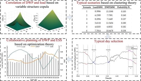
First, we discretize the phased copula model and generate a sample data of 96,000 × 2 dimensions. Next, set the number of typical scenarios to 6 and select the initial condensation point. Finally, use the K-means method to cluster the remaining discrete points and find the corresponding original quantiles.

According to the steps in Section 2.3,

Table 6. Quantile of DWP and load with probabilities in typical scenarios.

Scenario	Load (MW)	DWP (MW)	Probability PL
1	8.3986	15.3398	0.183
2	6.2500	7.7391	0.160
3	8.2094	7.1449	0.137
4	5.6118	12.5456	0.180
5	4.8205	6.8032	0.182
6	7.7814	10.6478	0.158

shows the generation results of typical scenarios.

It can be concluded from the results that each typical scenario has a similar incidence, which illustrates the rationality of dividing the initial points into six typical scenarios.

4.5. Capacity Planning of DWP

According to (7)–(9), the optimal solution of the objective function under the constraints of each scenario is obtained.

Table 7. Optimal DWP output and objective function values for each scenario.

Scenario	Probability	DWP (p.u.)	F(×104 RMB)
1	0.183	0.0883	1066.72
2	0.160	0.0648	889.63
3	0.137	0.0862	1015.56
4	0.180	0.0579	809.83
5	0.182	0.0495	686.76
6	0.158	0.0815	905.09

shows the results of capacity planning of DWP and the optimal value of the objective function without energy storage planning in each scenario.

If capacity planning of DWP is conducted based on the minimum load from scenario 5 in Table 6, the planning result will be 4.95 MW, which is conservative. This will obviously cause a large amount of wind abandonment. The selection with the maximum capacity planning of DWP from scenario 1 will also lead to loss of economic profit. Taking into account the wind power consumption of the typical scenarios above and economic operation, the final planning capacity is the weighted sum with each scenario probability, that is:

$$P_{DWG*}={\displaystyle \sum _{i=1}^k{P}_{DWG(i)}{P}_{L(i)}}=0.0706(\mathrm{p}.\mathrm{u}.),$$

(28)

where k is the number of scenarios, P_DWG(i) is the planning capacity of DWP under scenario i, and P_L(i) is the probability of scenario i. The final capacity planning of DWP is 7.06 MW.

4.6. Collaborative Capacity Planning of DWP and ESS

To maximize the consumption of wind power, it is necessary to employ the ESS so as to increase the planning capacity of DWP.

Based on the generation of typical scenarios, a typical schedule day is selected, and the collaborative capacity planning of DWP and ESS is examined based on the 24-h daily curve. In Figure 13, based on the $\pm 10\%$ fluctuation range of DWP and load in each typical scenario, several typical scenarios in Table 6 are included and marked in the typical daily curve.

Before optimization, the initial value of SOC is 0.6, and the initial state of ESS is discharge.

Table 8. Related parameters of DWP and ESS [33,35].

Parameter	Value
Cwt (RMB/kW)	4000
Csr (RMB/kW)	3500
Cd (RMB/kWh)	0.68
Cp (RMB/kW)	4000
Ce (RMB/kVA)	3500
Cyw (RMB/kW)	20
r (%)	8
T (Year)	10
T’ (Year)	15
Maximum charging/discharge power (MW)	150/150
Maximum/Minimum capacity (MWh)	600/10
Charging/discharging efficiency (%)	85/95

shows some specific parameters.

Based on the conditions above, fmincon optimization function in Matlab^TM is employed to solve the proposed nonlinear constrained optimization problem.

Under the premise of allowing some wind abandonment, the optimal power output of DWP and the state of SOC in the typical day are obtained and shown in Figure 14. The corresponding charging and discharging power of ESS in the typical day is reported in Figure 15.

Based on the optimal DWP planning and the states of ESS in the typical day, the final energy storage capacity planning is 4.63 MW, and the final DWP capacity planning is 12.07 MW. It can be concluded from this study that:

(1)

The optimal planning of DWP and the SOC of ESS change with the fluctuation of load in the typical day. When load is smaller than actual wind power output, ESS charges and stores the extra wind power. When load is larger than actual wind power output, ESS discharges and supplies power to the load.

(2)

The SOC of the ESS fluctuates within [0.1, 0.9], which meets the requirement of energy storage operation.

(3)

Compared with the case without ESS, the DWP planning value increases from 7.06 MW to 12.07 MW, with the study results indicating that with the participation of energy storage, it is conducive to increasing the consumption of DWP.

Moreover, the active power loss of the distribution network, the annual cost of the system is further compared with that before the installation of ESS in

Table 9. Capacity of DWP and economy before and after installing ESS.

	DWP (MW)	Network Loss Cost (104 RMB)	Average Annual Total Cost (104 RMB)
Without ESS	7.06	554.8	1066.7
With ESS	12.07	289.9	981.1

.

ESS can release power at peak load and it can absorb excess power when DWP output is higher than load. From Table 9, ESS can reduce the rate of wind abandonment, and the network loss cost is reduced with the collaborative planning of ESS, and the average annual cost is reduced with the benefited from time-of-day tariff in the distribution network.

The fluctuation of bus voltage is further studied and compared in the typical day. The voltage magnitude at some buses is lower than 0.95 in the case of without ESS installation, as shown in Figure 16, and the bus voltages all lie in the range of [0.95, 1.05] based on the collaborative planning of ESS as reported Figure 17.

Based on the comparison of Figure 16 and Figure 17, with the installation of the ESS, the voltage level is increased effectively at heavy load conditions. At the same time, the range of voltage fluctuation is reduced.

5. Conclusions

This paper proposes a DWP capacity planning method with participation of ESS optimization under multi-scenario conditions based on variable-structure copula and optimization theory. The conclusions can be reached as follows.

(1)

The variable-structure copula models of DWP and load are established based on two different time segment strategies. The average Euclidean distance of the strategies by month is 1.8864, which is smaller than the strategies by quarter. It is concluded that the variable-structure copula model with time segment by month is better able to fit the changes of the correlation structure between DWP and load and can capture the correlation at each segment more accurately.

(2)

The continuous correlation functions are discretized and typical scenarios of DWP and load are obtained by the clustering method. For each typical scenario, a feasible capacity planning model of DWP is established. In addition, the feasible optimal capacity of DWP is 7.06 MW, which is higher than the lowest active power demand of load. Therefore, the capacity planning model of DWP considering the correlation of DWP and load can effectively increase wind power consumption.

(3)

Furthermore, a collaborative capacity planning model for DWP and ESS is proposed. Study results show that, compared with the case without participation of ESS, the capacity of DWP planning was increased to 12.07 MW, and the consumption of wind power was efficiently improved. For economy, collaborative capacity planning of DWP and ESS can reduce the cost of network loss of the distribution network and the annual cost of the system; moreover, for reliability, it can effectively satisfy the lower voltage limit and reduce the range of voltage fluctuation.

Future work includes the investigation of time-varying copula model and multi-point integration of wind and storage system for DWP planning.

References

- Shu, Z.; Jirutitijaroen, P. Optimal operation strategy of energy storage system for grid-connected wind power plants. IEEE Trans. Sustain. Energy 2014, 5, 190–199. [Google Scholar] [CrossRef]
- Abdulgalil, M.A.; Khalid, M.; Alismail, F. Optimizing a distributed wind-storage system under critical uncertainties using benders decomposition. IEEE Access 2019, 7, 77951–77963. [Google Scholar] [CrossRef]
- National Energy New Energy. National Energy Administration Notice on Printing and Distributing the Interim Administrative Measures for the Development and Construction of Decentralized Wind Power Projects; National Energy Administration: Beijing, China, 2018.
- Huang, D.; Li, H.; Cai, G.; Huang, N.; Yu, N.; Huang, Z. An efficient probabilistic approach based on area grey incidence decision making for optimal distributed generation planning. IEEE Access 2019, 7, 93175–93186. [Google Scholar] [CrossRef]
- De Oliveira, K.L.M.; Penido, D.R.R.; De Araujo, L.R. Planning of the wind farm distribution network using heuristic methods. IEEE Latin Am. Trans. 2018, 16, 2917–2924. [Google Scholar] [CrossRef]
- Ehsan, A.; Yang, Q.; Cheng, M. A scenario-based robust investment planning model for multi-type distributed generation under uncertainties. IET Gener. Transm. Distrib. 2018, 12, 4426–4434. [Google Scholar] [CrossRef]
- Zheng, Y.; Dong, Z.Y.; Meng, K.; Yang, H.; Lai, M.; Wong, K.P. Multi-objective distributed wind generation planning in an unbalanced distribution system. CSEE J. Power Energy Syst. 2017, 3, 186–195. [Google Scholar] [CrossRef]
- Ouammi, A.; Dagdougui, H.; Sacile, R. Optimal planning with technology selection for wind power plants in power distribution networks. IEEE Syst. J. 2019, 13, 3059–3069. [Google Scholar] [CrossRef]
- Wang, G.; Xin, H.; Wu, D.; Ju, P.; Jiang, X. Data-driven arbitrary polynomial chaos-based probabilistic load flow considering correlated uncertainties. IEEE Trans. Power Syst. 2019, 34, 3274–3276. [Google Scholar] [CrossRef]
- Chen, J.; Yu, Q.; Li, Q.; Lin, Z.; Li, C. Probabilistic energy flow analysis of MCE system considering various coupling units and the uncertainty of distribution generators. IEEE Access 2016, 7, 100394–100405. [Google Scholar] [CrossRef]
- Sun, G.; Guan, X.; Yi, X.; Zhao, J. Conflict evidence measurement based on the weighted separate union kernel correlation coefficient. IEEE Access 2018, 6, 30458–30472. [Google Scholar] [CrossRef]
- Ouyang, J.; Li, M.; Zhang, Z.; Tang, T. Multi-timescale active and reactive power-coordinated control of large-scale wind integrated power system for severe wind speed fluctuation. IEEE Access 2019, 7, 51201–51210. [Google Scholar] [CrossRef]
- Wu, Y.; Lee, C.; Chen, C.; Hsu, K.; Tseng, H. Optimization of the wind turbine layout and transmission system planning for a large-scale offshore wind farm by AI technology. IEEE Trans. Ind. Appl. 2014, 50, 2071–2080. [Google Scholar] [CrossRef]
- Jiang, C.; Mao, Y.; Chai, Y.; Yu, M.; Tao, S. Scenario generation for wind power using improved generative adversarial networks. IEEE Access 2018, 6, 62193–62203. [Google Scholar] [CrossRef]
- Ehsan, A.; Cheng, M.; Yang, Q. Scenario-based planning of active distribution systems under uncertainties of renewable generation and electricity demand. CSEE J. Power Energy Syst. 2019, 5, 56–62. [Google Scholar] [CrossRef]
- Nelson, R.B. An Introduction to Copulas; Springer: New York, NY, USA, 2006; pp. 109–115. [Google Scholar]
- Ehsan, A.; Yang, Q. Coordinated investment planning of distributed multi-type stochastic generation and battery storage in active distribution networks. IEEE Trans. Sustain. Energy 2019, 10, 1813–1822. [Google Scholar] [CrossRef]
- Khalid, M.; Akram, U.; Shafiq, S. Optimal planning of multiple distributed generating units and storage in active distribution networks. IEEE Access 2018, 6, 55234–55244. [Google Scholar] [CrossRef]
- Xia, S.W.; Bu, S.Q.; Wan, C.; Lu, X.; Chan, K.W.; Zhou, B. A fully distributed hierarchical control framework for coordinated operation of DERs in active distribution power networks. IEEE Trans. Power Syst. 2019, 34, 5184–5197. [Google Scholar] [CrossRef]
- Liu, Y.; Xiao, L.Y.; Yao, G.D.; Bu, S.Q. Pricing-based demand response for a smart home with various types of household appliances considering customer satisfaction. IEEE Access 2019, 7. [Google Scholar] [CrossRef]
- Sklar, A. Fonctions de Répartition àn Dimensions et Leurs Marges; University Paris Press: Paris, France, 1959; pp. 229–231. [Google Scholar]
- Cui, M.; Krishnan, V.; Hodge, B.; Zhang, J. A copula-based conditional probabilistic forecast model for wind power ramps. IEEE Trans. Smart Grid 2019, 10, 3870–3882. [Google Scholar] [CrossRef]
- Papaefthymiou, G.; Kurowicka, D. Using copulas for modeling stochastic dependence in power system uncertainty analysis. IEEE Trans. Power Syst. 2009, 24, 40–49. [Google Scholar] [CrossRef] [Green Version]
- Ma, Z.; Chen, H.; Chai, Y. Analysis of voltage stability uncertainty using stochastic response surface method related to wind farm correlation. Prot. Control Mod. Power Syst. 2017, 2, 1–9. [Google Scholar] [CrossRef] [Green Version]
- Wang, Y.R.; Luo, Y.N. Research of wind power correlation with three different data types based on mixed copula. IEEE Access 2018, 6, 77986–77995. [Google Scholar] [CrossRef]
- Stephen, B.; Galloway, S.J.; McMillan, D.; Hill, D.C.; Infield, D.G. A copula model of wind turbine performance. IEEE Trans. Power Syst. 2011, 26, 965–966. [Google Scholar] [CrossRef] [Green Version]
- Holeňa, M.; Bajer, L.; Ščavnický, M. Using copulas in data mining based on the observational calculus. IEEE Trans. Knowl. Data Eng. 2015, 27, 2851–2864. [Google Scholar] [CrossRef]
- Hazarika, S.; Biswas, A.; Shen, H. Uncertainty visualization using copula-based analysis in mixed distribution models. IEEE Trans. Vis. Comput. Graph. 2018, 24, 934–943. [Google Scholar] [CrossRef]
- Chen, Z.; Li, S. CDO pricing using Archimedean copula with dynamic structure. In Proceedings of the 2014 International Conference on Management Science & Engineering 21th Annual Conference Proceedings, Helsinki, Finland, 17–19 August 2014; pp. 1121–1126. [Google Scholar]
- Wang, Y.; Luo, Y.; Dai, Z. Study and comparison of wind power correlation using two types of dataset. In Proceedings of the 2018 IEEE Power & Energy Society General Meeting (PESGM), Portland, OR, USA, 5–9 August 2018; pp. 1–5. [Google Scholar]
- Eryilmaz, S. Modeling dependence between two multi-state components via copulas. IEEE Trans. Reliab. 2014, 63, 715–720. [Google Scholar] [CrossRef]
- Sedghi, M.; Ahmadian, A.; Aliakbar-Golkar, M. Optimal storage planning in active distribution network considering uncertainty of wind power distributed generation. IEEE Trans. Power Syst. 2016, 31, 304–316. [Google Scholar] [CrossRef]
- Ma, M.T.; Yuan, T.J.; Chen, G.Y. Analysis of comprehensive economic benefits of energy storage participating in wind power auxiliary service. Power Syst. Technol. 2016, 40, 3362–3367. [Google Scholar]
- Jinlei, S.; Lei, P.; Ruihang, L.; Qian, M.; Chuanyu, T.; Tianru, W. Economic operation optimization for 2nd use batteries in battery energy storage systems. IEEE Access 2019, 7, 41852–41859. [Google Scholar] [CrossRef]
- Jiang, P.; Yuan, T.J.; Che, Y.; Liu, B. Research on capacity planning of the integration of decentralized wind and storage system. Power Capacit. React. Power Compens. 2018, 39, 138–146. [Google Scholar]
Figure 1.
The daily curve of DWP and local load demand.
Figure 2.
The system diagram of the DWP planning process.
Figure 3.
The modified IEEE 33-bus system.
Figure 4.
The comparison of marginal cumulative distribution and empirical distribution of DWP.
Figure 5.
The comparison of marginal cumulative distribution and empirical distribution of load.
Figure 6.
Binary frequency histogram of DWP and load in January 2018.
Figure 7.
(a) Probability density function of Clayton copula; (b) distribution function of Clayton copula.
Figure 8.
(a) Probability density function of Gumbel copula; (b) distribution function of Gumbel copula.
Figure 9.
(a) Probability density function of Frank copula; (b) distribution function of Frank copula.
Figure 10.
(a) Probability density function of Gaussian copula; (b) distribution function of Gaussian copula.
Figure 11.
(a) Probability density function of t copula; (b) distribution function of t copula.
Figure 12.
Empirical copula distribution function of DWP and load.
Figure 13.
The typical daily curve with several typical scenarios.
Figure 14.
Optimal output of DWP and the state of SOC in the typical day.
Figure 15.
The charging and discharging power of ESS in the typical day.
Figure 16.
The fluctuation of bus voltage in the typical day before installing the ESS.
Figure 17.
The fluctuation of bus voltage in the typical day after installing the ESS.