The Effect of Supercritical CO2 on Shaly Caprocks


Department of Petroleum Engineering, Western Australian School of Mines: Minerals, Energy and Chemical Engineering, Curtin University, Kensington, WA 6151, Australia
*
Author to whom correspondence should be addressed.
Energies 2020, 13(1), 149; https://doi.org/10.3390/en13010149
Submission received: 14 November 2019
/
Revised: 16 December 2019
/
Accepted: 23 December 2019
/
Published: 27 December 2019
(This article belongs to the Special Issue Development of Unconventional Reservoirs)
Abstract
:The effect of supercritical CO2 on the shaly caprocks is one of the critical issues to be considered in CO2 sequestration programs. Shale-scCO2 interactions can alter the seal integrity, leading to environmental problems and bringing into question the effectiveness of the program altogether. Several analytical studies were conducted on samples from Jurassic Eneabba Basal Shale and claystone rich facies of the Triassic Yalgorup Member (725–1417 m) in the Harvey CO2 sequestration site, Western Australia, to address the shale-scCO2 interactions and their effect on the petrophysical properties of the caprock. Shale samples saturated with NaCl brine were exposed to scCO2 under the reservoir condition (T = 60 °C, P = 2000 psi) for nine months and then tested to determine their altered mineralogical, petrophysical and geochemical properties. The experimental study examined changes to the mineralogical composition, capillary threshold pressure, and pore size distribution (PSD) of samples. The X-ray diffraction (XRD) results showed several changes in mineralogy because of rock-brine-CO2 reactions. Quartz, feldspars, kaolinite, and goethite were dissolved in most samples and muscovite, and halite were precipitated in general. Nuclear magnetic resonance (NMR), low-pressure nitrogen adsorption (LPNA), and mercury injection capillary pressure (MICP) tests indicate an increase in pore volume, except for relatively tighter, clay-rich samples. A reduction in capillary threshold pressures of samples after exposure to scCO2 is observed.
1. Introduction
The geosequestration of anthropogenic CO2 has been suggested as a solution for resolving the problem of increasing greenhouse gas emissions which are responsible for global warming [1]. CO2 is the major greenhouse gas, resulting from fossil fuel combustion for domestic and industrial purposes [2]. The injection of anthropogenic CO2 deep underground instead of releasing it to the atmosphere is the basic concept in this method [3]. CO2, under the storage condition of target reservoirs (below 800 m), is in the critical state (CO2 critical point: 31.8 °C and 7.38 MPa). Saline aquifers are the most common target for the injection of CO2, due to their abundancy and proximity to the source [4,5]. The excessive amount of CO2 in the geologic formation, which also contain water, modifies the chemical equilibrium of the existing system and induces a series of reactions. The interactions between rock-forming minerals, brine, and injected CO2 in deep brine aquifers alter the natural petrophysical properties of CO2 geosequestration sites [6].
The mitigation of ScCO2 into the subsurface initiates the CO2-water-rock interactions in geologic storage strata that, in time, render the pH of the environment into an acidic condition, which, in turn, is expected to be buffered by reactions with the silicate/oxide/carbonate phases. Increasing the pH with time, due to this buffering effect, may result in carbonates or other phases re-precipitating in the pore system that had been dissolved initially [7,8]. Even after pH buffering, due to carbonate dissolution, the acidity of the brine will still be sufficient to attack alumino-silicate minerals (e.g., clays and feldspars) [9]. Subsequently, such reactions are often followed by alterations to the petrophysical properties of the rock. Several laboratory investigations on mineral transformations in CO2 storage reservoirs indicated that some changes of caprock’s fluid transport properties and mineralogical composition may occur [10,11,12,13,14,15,16,17]). Credoz et al. (2009) suggested that potential pathways for CO2 leakage through the caprock could be induced as the result of geochemical alteration occurring along with the reservoir-caprock interface with the CO2-brine mixture [18]. However, Busch et al. (2008) suggested that the depth of influence of such reactions is only limited to the lower part of the caprock in the vicinity of the CO2 plume [7].
CO2 containment and long-term safety for both humans and the environment are crucial factors to consider before implementing large scale CO2 storage. Containment of the injected CO2 for hundreds to thousands of years by trapping mechanism determines the success of geologic CO2 sequestration as a large-scale carbon management strategy. Interaction of scCO2-shale and the subsequent shale alteration can cause seal failure and leakage of CO2 to the upper formations and the atmosphere [9]. Assessing the CO2-rock interaction is an important part of such studies, as these potentially affect physical properties. There have been few studies to address the caprock sealing properties’ variation during the geosequestration of CO2 [8,11,12,14,15,19,20,21,22,23]. This study aims to assess the directions of the geochemical reactions and the petrophysical alteration as a result of dissolution/precipitation mechanisms in potential shaly caprock in the South West Hub, Western Australia under in situ conditions. This research is aimed at reducing uncertainties in the efficacy of shaly caprocks in a CO2 storage system.
Laboratory experiments of rock samples with CO2 and brine have been frequently applied as a strategy for studying the potential geochemical reactions. Most of the existing experiments have been conducted for less than three months and at very high temperatures to increase the chemical reaction rates. Some drawback of such batch experiments cannot be fully resolved, including short laboratory time scales and the increase of reactive surface area and reaction temperature, variation in the brine/rock ratio and the potential formation of experimental artefacts during reactor depressurisation and cooling [24]. However, the mineral-brine-CO2 reaction is a long-term process, and short time-scale experiments are less accurate in predicting field conditions. Therefore, there is a necessity for experiments conducted over long-term timescales at low temperatures to represent actual reservoir conditions [1].
Short laboratory time scales of batch experiments are one drawback, which is why we tried to expand the reaction time to the maximum possible of nine months as opposed to several weeks to several months, as in previous studies. Elevated temperature is one other drawback which we avoided by selecting the in situ temperature of 60 °C. Samples were in different forms according to the requirement of each method. Core plugs, disks, rock fragments, and powdered samples were used in the reactor to avoid unnecessary changes to the surface area.
Ten samples out of the fifteen original samples were chosen to be used in this research. In this study, several methodologies for assessing CO2-rock interactions are discussed and applied. These ten samples were analysed with X-ray diffraction (XRD) and low-pressure nitrogen adsorption (LPNA) methods in powder form. Only five plugs were recovered for nuclear magnetic resonance (NMR) measurement. The same samples were also analysed with the mercury intrusion porosimetry (MICP) method. The overall experimental procedure started with testing the samples in their original state, then exposing them to scCO2, and finally testing them again after the exposure phase. The NMR samples were also tested midway through the exposure phase. The results show changes in mineralogical composition and alterations in pore size distribution, total pore volume, average pore width, total pore surface area, and capillary pressure of the samples, because of the reactivity between scCO2-brine-minerals. The porosity increase was more significant in larger pores and samples which lacked clay minerals (kaolinite). The direction of the changes was to enhance the transport properties, as the pore volumes increased generally, and capillary threshold pressure decreased. Future works include a geochemical reaction path modelling to simulate the results of this study, and to further supplement the results of this study for longer periods.
2. Geological Setting
There has been a focus on the Carbon Capture and Storage (CCS) program in Australia in recent years, as the country is one of the top twenty countries in CO2 emission per person. With its stationary energy-intensive industries, Australia is predicted to contribute to 20% of CO2 emissions by the end of 2020, Currently, several projects have been proposed or already established in Australia for CCS purposes, such as South West Hub, CarbonNet, Otway (Victoria), Surat, Gippsland (SA), and Gorgon [25,26].
In Western Australia, two suitable mainland locations for the geosequestration of carbon dioxide have been identified. Carbon Capture and Storage in Gorgon and Borrow Island in the North West are active projects. The South West Hub project has been introduced as a potential mainland location for the geosequestration of carbon dioxide. This potential CCS system has suitable storage capacity in its saline aquifer and efficient seal properties in the shaly caprock. In addition, the area is located relatively close to the biggest CO2 emitter of the state, the Kwinana Power Plant. It is planned to collect CO2 from several industrial emitters, where the injection masses are expected to be in the order of 6.5 million tons per year for the 40 years of project activity [27].
The potential geosequestration site is in a deep saline aquifer within the Lesueur Sandstone. A total of four wells have been drilled in the Harvey region to investigate the suitability of the Lesueur Formation of Southern Perth basin for storage of industrial-scale CO2 emissions. The results have identified significant differences in sedimentology and petrophysical properties of the Upper and Lower Members of the Lesueur Sandstone. The Lower Member of the Triassic Lesueur (Wonnerup) is a laterally extensive and thick layer of sandstone which represents the targeted reservoir, whereas the Upper Lesueur (Yalgorup) is far more heterogeneous, due to the mixed nature of the mudstone intervals and the thick continuous clean sandstone succession [28].
The targeted seals are identified in a series of rock baffles in the Triassic Yalgorup Member (Triass) and a thick interval of paleosol section (Jurassic Basal Eneabba Shale). The Yalgorup Member consists of mixed-thickness, interbedded high- to low-energy channel-fill facies, and swampy/overbank deposits, and paleosols. The Wonnerup Member consists of thick, continuous, high-energy channel-fill facies, with minor intercalations of moderate- to low-energy channel-fill/stacked rippleforms and rare swampy deposits. This is an ideal lithology for a CO2 reservoir [27].
3. Samples and Methods
3.1. Samples
Relatively fresh samples of shale intervals were selected from the Harvey3 well cores in Perth’s Core Library, Western Australia, to achieve the objectives of this study. A total of fifteen core samples from Eneabba Basal Shale and claystone rich facies of the Yalgorup Member (Lesueur Sandstone), depth ranging from 741 to 1218 m, were collected in September 2016.
The shale samples were characterised with a full suite of non-destructive petrophysical methods. The samples were analysed before and after they were dynamically exposed to supercritical CO2 under in situ reservoir conditions. X-ray diffraction (XRD) analyses were used to examine the compositional changes of the seal rock mineralogy. XRD analysis indicated whether any dissolution or precipitation has taken place [29]. Pore size distributions were measured using low-pressure nitrogen adsorption [7], and nuclear magnetic resonance (NMR) [30,31,32] methods. Low-pressure nitrogen adsorption measured the surface area and pore volume to check the occurrence of any changes to this critical rock parameter [33,34]. The pore size distribution was also obtained from the mercury injection capillary pressure method. MICP also provided more data, such as the threshold pressure and the height of the column of CO2.
3.2. Exposure to scCO2
The selected shale samples were required to be saturated with synthetic brine before being placed into the pressure–volume–temperature (PVT) cell at storage conditions and exposed dynamically to scCO2 for nine months. Simplified artificial pore water (brine) of 30,000 ppm (512 mmol/L NaCl) was prepared from ROWE ultrapure water and ROWE NaCl (CS10307) and used for all the batch reactions. This concentration was chosen to be equivalent to the available groundwater data of the Harvey3 Lesueur formation fluid sampling from the Rockwater Hydrological and Environmental Consultants Report [35]. This synthetic water chemistry was selected so that there would be minimal risk of damage to the core materials before exposing them to scCO2. Also, the dissolution process was encouraged by simple NaCl brine as it lacked the divalent cations, which have a pH-buffering effect and decrease the acid-induced reactions [36]. On the other hand, the cations needed for mineral precipitation can only be derived from the reactions with rock-forming minerals, instead of brine [12]. The selected shale samples were pressure-saturated at 2000 psi with 30,000 ppm NaCl solution before being placed into the PVT cell.
Shale samples in various forms of core-plugs, small rock fragments and crushed rock were tested in this study for pore accessibility and conformance with measurement methods [37]. We placed the selected shale samples into a PVT cell (Figure 1) under the reservoir condition of 2000 psi and 60 °C, related to the deepest sample recovered from the depth of 1400 m, for nine months. During the exposure, high-purity (99.9 mole%) scCO2 mixed with deionised water was injected continuously using a high-accuracy continuous pump with a constant rate into the PVT cell. The high-performance liquid chromatography (HPLC) injection pump (SHIMADZU LC-20AT) allowed the pressure and flow-rate values to be set at 2000 psi and 0.7 cm3/h (i.e., 0.01 mL/min), respectively, which could be controlled and recorded with the accuracies of 1 psi, and 0.001 mL/min, respectively. The injection rate must be realistic so that we can expect the same experimental results as the real-life injection process. We adopted the same method of rate calculation as [38]. The accumulator connected to the input of the samples cell was filled with CO2 and pressurised with an air-driven compressor about every 40 days.
To make the CO2 saturated with water, 50 mL of water was injected inside the accumulator initially. Under the high pressure and temperature of the cell, water dissolved in the scCO2 and made it wet. The outlet end of the samples cell was connected to a Swagelok KPB back-pressure regulator, which maintained the pressure inside the cell equal to 2000 psi (in situ pore pressure). The temperature inside the cell was set to 60 °C and maintained using a Proportional-Integral-Derivative (PID) Temperature Controller (omega CSi8DH) and heating jackets (omega SRFG series) with an accuracy of 0.04 °C. The accumulator and exposure cell with the attached heating jacket were wrapped in insulation pads to minimise the temperature fluctuation. All wetted parts of the apparatus are made from Hastelloy, super duplex stainless steel or titanium to minimise any fluid contamination or damages caused by corrosion when exposed to highly corrosive materials (e.g., carbonated water or high salinity brine) under high pressures and temperatures for a prolonged period. At the end of the exposure, the pressure and temperature were reduced gradually to room conditions and samples were examined again to assess any rock chemical and petrophysical alterations.
3.3. Experimental Approach
The composition of the shale samples in the unreacted sample was measured by XRD before conducting the batch experiments. For XRD analysis, the samples were crushed, homogenised and divided into two aliquots to avoid the heterogeneity of samples effecting the results. Each patch was then mixed with methanol and further ground in a micronizing mill to around 1–5 µm. The solution was dried overnight at 40 °C in a fume cupboard. Once the samples had dried, they were packed in sample holders and an XRD pattern was obtained. X-ray diffraction (XRD) analyses of the samples were performed using a Bruker D8 Advance automated powder diffractometer with Bragg-Brentano configuration at the John de Laeter Centre of Curtin University. It used a LynxEye detector and a copper X-ray tube at 20 kV and 5 mA. The whole-rock samples were analysed over an angular range of 7 to 120 degrees 2Ɵ. The instrument was complemented with Bruker DIFFRAC EVA software for search/match analysis, and the XRD quantitative results were calculated using the Rietveld method in the comprehensive full pattern data analysis programme, TOPAS.
The 2 MHz Magritek bench-top laboratory NMR spectrometer was applied to record T2 relaxation time spectrum of shale core plug samples before and after exposure to CO2 to estimate the porosity and pore size distribution. The magnet operated at a stable temperature of 30 °C and atmospheric pressure, with a frequency of approximately 2 MHz. Shale core plugs of 1.5-inch diameter and about 1.5-inch length were measured using a P54 probe, which allowed a minimum CPMG (Carr-Purcel-Meiboom-Gill) echo-spacing of 100 µs [39,40]. In this work, the T2 relaxation time measurements were conducted on six types of samples. Dry samples, as received from the core library, and then the samples saturated with 30,000 ppm NaCl brine were measured. The T2 relaxation time measurements were conducted again after samples were exposed to scCO2 for four and nine months, both in a dry and saturated state.
The BET surface area and pore size distribution of the core samples were determined by the low-pressure nitrogen adsorption method based on the quantity of gas that adsorbs as a single layer of molecules on the rock surface. Approximately 0.6 g of each sample was loaded into a glass sample tube. To ensure a surface free of traces of gas and water molecules, it was necessary to remove moisture content and degas the samples before pore structure analysis [41]. The samples were degassed for 8 hours at 110 °C before starting the main analysis. Finally, the nitrogen adsorption and desorption isotherms were collected at a constant temperature of 77 K (−196 °C) using a Micromeritics® TriStar II 3020 apparatus [42]. The adsorption and desorption isotherm curves were measured using between 40 and 60 points. The amount of gas adsorbed depended on the adsorbent and the temperature and pressure, and was measured by the instrument at different relative pressures (P/P0) where P is the gas vapour pressure in the system and P0 is the saturation pressure of the adsorbent. The adsorption isotherm is the point by point measurement of the quantity of nitrogen adsorbed against the equilibrium pressure, while desorption isotherms are the measured quantity of nitrogen from the sample as the relative pressure is lowered [42]. Pore size distributions (PSD) were obtained based on the density functional theory (DFT) model in this study. The DFT model provides a much more accurate approach for pore size analysis of micropores and even smaller mesopores [38]. It overcomes the oversimplified approach of previous methods which underestimated the pore sizes and yields more reliable pore size results over the full nanopore range by describing the adsorbate configuration at the molecular level [43,44].
The MICP experimental data were measured using a Micromeritics Autopore IV 9500, Capillary pressure curves were collected for pressure points in the range 0.5–60,000 psi, which allowed for the assessment of equivalent pore sizes between 3 and 3.5 × 10⁵ nm approximately. Ten small rock fragments weighing 1.8–4.1 g for five samples were used for tests. Like for low-pressure adsorption measurement, the samples were evacuated before the test to remove moisture and possible gas content. Before mercury was injected into the chamber, the shale samples were degassed at a 25 μmHg vacuum pressure for 10 min. In all cases, the experimental data were collected using a reference equilibration rate of at least 0.001 μL/g/s with a mercury filling pressure of 0.53 psi. The pore throat sizes were calculated based on the Washburn equation [45] for a mercury surface tension of 485 dynes/cm, with an advancing contact angle of 130°.
PC = capillary pressure (psi), γ = interfacial tension (dynes/cm), Ɵ = wetting angle, d-pore diameter (microns), C = 0.145 (constant to convert to psi). Considering ϒHg/air = 485 dynes/cm and ƟHg/air = 130°, we have the following equation:
4. Results
4.1. Mineralogical Changes
Bulk X-ray diffraction analysis was performed on selected samples to characterise their mineral composition before and after nine months. The collected samples were quartz-rich mudstone with significant Illite/mica and kaolinite and sub-dominant feldspars (Table 1). The average detrital quartz and feldspar grains were 30 and 9 weight percent, respectively. The major clay types were kaolinite and Illite-mica, with an average of 27% and 31%, respectively. Samples H1, H6, H9, H10, H11, and H16 were the clay-rich samples with a clay content of more than 60%. The most quartz-rich sample was H8, with a maximum of 56.7%, and the highest amount of kaolinite was in samples H1 (43%) and H11 (45%). Minor amounts of goethite, pyrite, hematite, and calcite also occurred in some of the samples analysed. Sample H1 had the highest amount of goethite (9%) among the samples; a lesser amount of goethite (<2%) was found in most of the samples. The samples were free from carbonates. Only a minor amount of hematite and pyrite was found in some samples.
Table 1 summarises the quantitative amount of minerals in each sample before and after four and nine months of exposure to scCO2. The quartz content is constantly reduced in all the samples, which is a sign of quartz dissolution. However, an increase in the amount of quartz is attributed to the dissolution of feldspar and clay minerals. Microcline is decreased in some samples (H4, H9, H13, H14, and H15) and increased in samples H1 and H2 after exposure. For samples H5, H8, and H10, there is a mixed trend in the amount of microcline. Albite and anorthite rich H4 show a decrease in both minerals post-exposure, but a sharp increase in albite amount in H2. A significant increase in albite and microcline content is observed in sample H2 after nine months.
For clay minerals, kaolinite decreases, and muscovite increases in most samples (H1, H2, H4, H9, H10, and H14). The clay content in the samples follows an interesting trend. In the samples where the kaolinite content is continuously decreased, an increase in muscovite content is constantly evident. Halite is increased in all samples as a result of brine desiccation. Carbonate minerals, which are of great significance in the mineral trapping of CO2 through the reaction with magnesium and calcium ions provided by silicate minerals, are mostly absent in the samples analysed.
4.2. Nuclear Magnetic Resonance
Nuclear magnetic resonance (NMR) experiments were carried out on a low field Magritek bench-top Rock Core Analyzer, located in the Department of Petroleum Engineering at Curtin University. A total of seven core plugs were recovered from the samples received from the core library. The other samples were either too soft or were broken, and plugs could not be taken from them. The study involved six types of T2 relaxation time measurements: (1) dry state (as received samples from core store) before exposure to scCO2 (Before_Dry); (2) brine-saturated state before exposure to scCO2 (Before_Sat); (3) after exposure to scCO2 for four months (4M_Dry); (4) brine re-saturated state after exposure to scCO2 for four months (4M_Sat); (5) after exposure to scCO2 for nine months (9M_Dry); and (6) brine re-saturated state after exposure to scCO2 for nine months (9M_Sat). Sample H8 and H10 collapsed later during saturation stages.
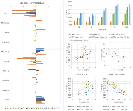
Figure 2 lists the NMR porosity for the samples analysed. There is a notable increase in porosity for the samples that were exposed to scCO2. The average NMR porosities are 7.62%, 19.55%, 14.44%, 20.68%, 14.76%, and 20.46% for Before_Dry, Before_Sat, 4M_Dry, 4M _Sat, 9M_Dry, and 9M_Sat respectively. There is an increase in the average porosity of samples exposed to scCO2.
Figure 3 illustrates the combined T2 distribution for all Before_Dry, Before_Sat, 4M_Dry, 4M_Sat, and 9M_Dry core plugs respectively. The T2 distributions of the Before_Dry samples, which is peaked at the lower T2 region, illustrate a shape that corresponds to clay surface water. After the saturation, the dominant peak of the T2 distribution of the Before_Sat state is shifted toward higher T2 times, which likely corresponds to a combination of both clay surface water and capillary pores. The T2 distribution of the samples after exposure to scCO2 show a slight reduction in the height of dominant peak.
Some of the water in the samples was removed after exposure to scCO2 (Figure 3) which resulted in reductions in the NMR signals. Exposure to scCO2 could induce rock dehydration in the samples.
The bimodal T2 distribution observed in the saturated samples is indicative of clay surface water and water in the interstitial pores. Samples H10 and H8 failed during saturation process and could not be analysed.
4.3. Low-Pressure Nitrogen Absorption
A low-pressure nitrogen Adsorption (<18.4 psi, 77 K) test was applied on ten samples from Harvey3 before and after they were exposed to scCO2. The values for the surface area and pore volume and their distribution along the pore width are reported and compared here. The pore size (diameter) is calculated from these values and included in this study. The results indicate some significant changes in the nanopore structure system of the samples after scCO2 and shale interactions. However, the variation trend of the pore structure parameter was quite different after exposure to scCO2, which is related to the discrepancies in the mineralogical and geochemical properties of the samples.
Table 2 and Table 3 summarise the collected results from low-pressure adsorption measurement for the samples before and after exposure to scCO2. The average pore width for the Before and After data was found to be 3.90 and 4.5 nm, respectively. The average pore volume obtained from LPNA tests for Before and After samples is about 4 and 4.4 cm3/100 g, which is characterised by a very high contribution of the mesopore size, 76.63% and 83.48% of total porosity, respectively. The average BET surface area is found to be 43.42 m2/g, and 39.42 m2/g (Before and After). Figure 4 compares the total pore volume in samples studied. Figure 5 and Figure 6 compare the BET surface area and pore size of the analysed samples before and after exposure to scCO2.
The low-pressure nitrogen adsorption analysis shows that the pore structure changed after the shale samples were exposed to scCO2. For most of the samples studied there was an increase in the pore volume (H5–H15). However, there was a decrease in the pore volume for samples H1, H2, and H4 (Figure 4). The porosity increased significantly in samples H5, H9, and H13, where the post-exposed pore size distribution (PSD) curve sits on top of the preexposed curve along the whole pore width range (Figure 7). An average increase of 21% is observed in samples H8, H10, H14, and H15, where the post-exposed curve is increased only in the lower pore width range (<20 nm).
Figure 8 and Figure 9 show the pore volume distribution of the micropores, mesopores, and part of macropores before and after the exposure. As can be seen for H8 and H10, there are no significant changes in the PSD after exposure to scCO2 for pores larger than 20 nm. The pore volume has slightly increased for pores smaller than 20 nm of width in these two samples. Whereas, for samples H5, H9, and H13, the PSD shows an increase in the pore volume in the whole pore size spectrum, but the general trend follows the PSD of the sample before exposure to CO2. Samples H14 and H15 show a significant increase in pore volume in pore widths smaller than 20 nm, which is followed by a pore volume decrease in pores larger than 20 nm. Samples H1, H2, and H4 have a more complex increase/decrease trend. They show a large decrease in the pore volume of the larger pore size range (> 18 nm) after exposure to CO2, which results in total pore volume decrease in these three samples (Figure 4) In pore sizes smaller than 18 nm, a mixed pattern is observed. Samples H1 and H2 show an increase then decrease, but sample H4 shows a decrease then increase in pore volume in the lower mesopore range.
In summary, pores with a diameter of 18–20 nm are the turning point for most of the samples. In the first three samples, the substantial decrease of pore volume above this turning point results in an overall pore volume reduction of samples. For the remaining samples (H5 to H15), the total pore volume is increased, but the contribution of pore sizes above or below the turning point is different. Pore size below the turning point plays the deciding role in samples H8, H10, H14, and H15, as the pore volume increase in this range is so large that it either covers the reduction in larger pore sizes, or there is no pore volume reduction in the larger pore size range. On the other hand, in samples H5, H9, and H13, the pore volume is increased in the whole 2–100 nm range and no turning point is observed.
In general, the surface area was increased in most of the samples after exposure, especially in mesopore size ranges. As can be seen in Figure 5, the BET surface area in samples H1, H2, H5, H8, H9, and H13 is increased, and in samples H4, H10, H14, and H15 is decreased after exposure. Among the samples, H8 has the lowest surface area, which is the most quartz-rich sample (57%). Samples H4, H10, H14, and H15 have a surface area in the range of 50–70 m2/g and samples H1, H2, H5, H9, and H13 have a surface area in the range of 30–40 m2/g. The pore diameter was calculated using the volume to surface area ratio and shows the same trend as pore volume changes. The calculated average pore diameter follows the same decreasing/increasing trend of pore volume, except for sample H4 after exposure to CO2 (Figure 6).
4.4. Mercury Injection Capillary Pressure
Table 4 presents the results obtained from MICP measurements on five samples before and after exposure to scCO2. Variation can be observed, comparing the petrophysical parameters in the tested samples. The porosity is increased in post-exposed samples H5, H9, and H13, and decreased in H1 and significantly decreased in H2. The pore areas in samples H1, H2 and H5 are decreased after exposure and increased in samples H9 and H13. The pore diameter in all the samples is enhanced after the exposure.
Porosity ranges of 9.59–14.09% for the Before samples and 4.17–18.53% for the After samples were recorded. The porosity was reduced for samples H1 and H2, from an average of 10.12% to 6.90%, but was enhanced from an average of 12.72% to 15.42% in the case of samples H5, H9, and H13. The general peak pore throat diameter of samples H1 and H2 show Before at 10.62 nm and After at 13.80 nm, smaller than samples H5, H9, and H13, which have values of 21.10 nm and 19.10 nm for the before- and after-exposure samples respectively (Figure 10). The average peak diameter of 10.62 nm was increased to 13.80 nm after exposure for samples H1 and H2. However, the higher average peak diameter of 21.10 nm for the before-exposure samples H5, H9, and H13 was decreased to 19.10 nm after the exposure.
Capillary pressure curves (Figure 11) summarize the relationship between the pressure applied to the samples at different stages and the volume of intruded mercury for each tested sample. Samples H1 and H2 have sigmoidal capillary pressure curves. Samples H5, H9, and H13 show distinctly bimodal pore-size distributions. All the samples exhibited 100% mercury saturation close to 60,000 psi. The highest entry pressures are observed for samples H1 and H2, whereas H9 display the lowest ones. Samples H1 and H2 are likely to have the most uniform pore size distributions, due to the more abrupt increment at low normalised mercury saturation, without further visible changes to the rate of intrusion (Figure 11). Since most of the intrusion occurs at higher pressures, H1 and H2 are also presumed to have the largest proportion of narrow pore sizes. This is verified by pore size distribution curves in Figure 10. In contrast, the more stepwise intrusion observed in the H5, H9, and H13 curves (Figure 11) is indicative of significant compression beyond the initial entry point, which is related to the presence of a wider and continuous range of pore sizes. The capillary pressure curves of after exposure samples in Figure 11 show a smoother slope. The intrusion of CO2 into the samples alters the pore sizes and pore throats in the samples, resulting in mercury intrusion starting at lower pressures compared with the before exposure samples.
The pore size distributions of the samples (Figure 10) demonstrate a dual trend. The first two samples exhibit narrow-distributed modals with higher peak values. A major throat size in the range of 6–18 nm is observed for samples H1 and H2; larger mesopores are very limited in terms of volume. The other three samples (H5, H9, and H13) demonstrate lower peaks and a wider range of pore throats spreading in the mesopore and macropore range.
In this work, the MICP threshold pressures for shale samples have been determined graphically at the point of inflection in the cumulative curves upon which the first rapid increase is observed. The same trend as capillary pressure curves and pore size distribution is also observed in the threshold pressure, where the two first samples have the highest and the other three samples have the lowest threshold pressure. However, after exposure to scCO2, samples H2 and H5 show the greatest decrease in their PThreshold of 72% and 83%, respectively, where all the samples’ threshold pressures are decreased. The height of the CO2 column is calculated assuming a contact angle of 130° and a Hg surface tension of 485 dynes/cm (Table 5 and Figure 12).
5. Discussion
Assessing CO2-rock interaction is an important part of seal integrity studies, as these potentially affect physical properties through highly coupled processes. The driving process of CO2-rock interactions includes dissolution of CO2 in brines, acid-induced reactions, reactions due to brine concentration, clay desiccation, pure CO2-rock interactions and reactions induced by other gasses than CO2 [9]. The observed changes in the petrophysical properties of the after-exposure samples are generally attributed to the three mechanisms of mineral dissolution, mineral precipitation and physical compaction [46]. The fine migration of susceptible minerals such as kaolinite is another important mechanism which can alter the properties of rock samples. The migration of clay fines generated and released by mineral dissolution is believed to have occurred in the exposure experiment conducted in this work. The occurrence and the extent of the effects of these mechanisms on a sample depend on the exact mineral composition, presence of core-scale heterogeneities and the original textural features of the sample and therefore, may vary from one sample to the next. Much of the discussions presented in the upcoming sections of this section are to determine how CO2-induced dissolution and precipitation reactions affect the pore space evolution and thus the physical properties of after-exposure samples, as revealed by the complementary measurements conduced.
5.1. The Effect on Mineralogy
The XRD analysis of the original caprock samples showed that samples H8 and H13 are quartz-rich, samples H1, H9, H10, and H15 are clay-rich (total clay > 60%), and samples H2, H4, H5, H13, and H14 have more clay content than quartz. The siliceous samples investigated in the current study are marked by a strong component of clay minerals, with up to 75% kaolinite and Illite. Samples are rich in both kaolinite (average: 26% and maximum 43%) and Illite (average: 29% and maximum 42%). Quartz content is 33% on average, with a maximum of 59%. The dominant feldspar in the samples is microcline (average 7% and maximum 10%). Samples H14 and H15 originated from the Eneabba shale formation, and samples H1–H13 originated from the same formation (Yalgroup member of Lesueur formation), but different localities. The different mineralogical composition of the samples leads to different reaction responses to the CO2-brine and brine systems.
XRD analysis of samples was carried out to measure the exact weight percentage of each mineral phase. The results were compared to the after-exposure results to monitor any changes in the amount of mineral phases. The X-ray diffraction (XRD) results show several changes in mineralogy because of rock-brine-CO2 reactions (Figure 13). Quartz, kaolinite, and goethite were dissolved in most samples and muscovite and halite were precipitated in general. Feldspars showed mixed behaviour across the samples.
Previous experimental work [11] showed some reactions occurring on a measurable time scale only at high temperatures of 200 °C. Other works [16] noted only a limited reaction of CO2 with pure mineral phases (anorthite and glauconite) at 50 °C and 150 °C and a low pressure. Changes in caprock fluid transport properties may happen regardless of the extent and scale of the mineralogical composition alteration. Wollenweber et al. (2010) reported carbonate dissolution and re-precipitation, leading to the alteration of shaly caprock transport parameters. In this case, no detectable mineral alterations were observed. The loss of quartz [47], feldspars [14], kaolinite [18], and chlorite [21] has been reported in other studies, resulting in an increase in porosity and opening up pore throats, leading to an increase in permeability.
The observed mineralogical alterations can be explained by the generation of carbonic acid (H2CO3). Changes in pH control the dissolution of minerals, release of chemical species, and formation of new compounds and minerals [7,8,10,17,48,49]. In the absence of calcite, reactive minerals such as feldspars, kaolinite and chlorite start to dissolve. The dissolution of these minerals releases Si, Al, Na, K, Fe, and Ca, which can form new compounds. The dissolution of feldspars and kaolinite results in the formation of muscovite/Illite.
The decrease in the quartz content of the samples, observed in previous experiments, is attributed to the dissolution of quartz itself. Rathnaweera et al. (2016) reported significant quartz dissolution under the 40 °C after a 1.5-year interaction with scCO2 and suggested that over a short period and under low temperature, quartz dissolution is too minor to be observed [50]. Szabó et al. (2016) also reported moderate dissolution of quartz, however in durations ranging 28–57 days [24]. Kaszuba et al. (2003) also observed dissolution of quartz along with oligoclase and biotite dissolution during their batch experiment at an elevated temperature and pressure (2000 °C and 200 bars) [11]. Other cases when quartz content was increased have been reported in other studies [22]. In such cases, the additional quartz is the product of the dissolution of other minerals such as feldspars and clay minerals. In an experiment with two types of shale caprocks, Alemu, et al. (2011) reported no major mineralogical alteration in the case of clay-rich shale, whereas in the case of carbonate-rich shale, plagioclase and clay minerals were dissolved, carbonates dissolved and re-precipitated, and smectite was formed [51]. Credoz et al. (2009) used purified clay minerals to evaluate their reactivity and found kaolinite to be the most reactive clay mineral in the long-term experiments [18].
Carbonate precipitation, such as the precipitation of dawsonite, siderite, calcite, dolomite, and magnesite, has been reported in several studies [52,53]. However, carbonate formation was not observed during this study. Since the shale sample used in this experimental study did not contain any carbonates and a very limited amount (2%) of Ca-feldspar in just one of the samples, a potential source for Ca was not available to form calcite and kaolinite assemblage. Also, low cation concentrations with an acidic pH were observed, which showed that dissolution prevailed over carbonate precipitation [17].
The formation of halite was interpreted as an experimental artefact. NaCl precipitated from Na and Cl coming from the solution, since the solid was not rinsed with deionised water before analysis [18].
5.2. The Effect on Petrophysical Properties
The low-pressure nitrogen adsorption method showed a slight increase in porosity observed in seven out of ten samples (Figure 4), except for samples H1, H2, and H4. Samples recorded a pore volume range of 1.7–5.7 cm3/g before exposure, which was changed to 2.1–6.4 cm3/g after exposure to CO2. There was an average 1.17 cm3/g increase in the pore volume of ten samples and an average 1.4 cm3/g decrease in the pore volume of three other samples tested.
The porosities were also estimated with the MICP and NMR methods for five samples. Samples H1 and H2 recorded a reduction in their porosity in both of these methods and samples H5, H9, and H13 show an enhancement in their porosities. The MICP porosities range is 9.6–16.3% for pre-exposure samples and 4.6–19.1% for after-exposure samples (Table 4). There was an average 2.7% increase in MICP porosity for three samples and an average 3.2% decrease in MICP porosity for two other samples tested.
The NMR porosities were measured in both dry and saturated states. The dry samples before exposure (as received) had porosities in the range of 6.35–9.67% and the range of 9.67–19.38% after four months of treatment and 10.36–19.08% after nine months of CO2 treatment. NMR porosities in saturated states are generally higher than dry states and their ranges for before, after four months, and after nine months of CO2 exposure are 14.90–24.55%, 12.12–26.93%, and 13.20–26.79%, respectively (Figure 2). While the NMR porosity of samples in the dry state increased across the sample by about 7.7%, the NMR porosity of saturated samples increased by an average 3% in three samples and decreased by an average 1.7% in two other samples tested. The increased porosity after the initial saturation stage is simply because the NMR method measures the response of hydrogen nuclei and then converts it to porosity. The received samples from storage were relatively dry and showed smaller porosities, which was significantly increased after the saturation. Each following exposure to CO2 reduced the porosities because of the evaporation of some of the water content. The following re-saturation stages did not increase the porosity as much as the initial saturation because the samples contained much of the water from the first saturation stage.
The received samples have a systematic monomodal distribution, with a relaxation time (T2) centred around 0.3–0.7 ms. After saturation, the previous population showed a shift toward a longer T2, centred between 9–1.6 ms, except for samples H1 and H2 which stayed centred between 0.33–0.46 ms. This first population is defined as the short relaxation time. A second population defined by long relaxation time was also recorded for the samples at around 13.5 ms. This second population is more likely the effect of the macropores filled by brine during the saturation process. The saturated samples show porosity values significantly higher than partially saturated samples.
The average pore width results of the LPNA method show an increase in most samples (H5, H8, H9, H10, H13, H14, and H15 and a decrease in three samples, H1, H2, and H4 (Figure 6). The average pore width range according to this method is 2.9–6.9 nm for pre-exposure samples, which is changed to 3.3–5.8 nm after exposure. However, the MICP average pore width is increased across all samples. The average pore diameter range of before-exposure samples is 11.3–22 nm, and for after-exposure samples the range is 12.7–28.1 nm (Table 4).
The leaching of the mineral constituents of the shale is the main reason for porosity increase. Mineral dissolution and precipitation can induce changes in porosity and permeability. In this study, an exposure period of nine months was selected, based on the reaction time required to complete the kinetically slow reactions of existing minerals with CO2 and brine to identify the fate of these major rock minerals. However, the timescales required to complete the reactions are certainly more than one year, up to hundreds or even thousands of years [54,55]. Therefore, considering the time frame available for this study and in order to record the maximum impact possible, nine months was selected as being a reasonable period for the CO2-brine-rock interactions. However, this period is not nearly enough to capture all the possible mineral reactions that occur in CO2 and brine environment, such as precipitation of feldspars and secondary precipitation of calcite and quartz. Therefore, it would be possible to see the dominant reactions such as the initial dissolution of quartz and kaolinite and the salt drying-out effect [50]. The significant increase in porosity observed in most experimental samples would potentially deteriorate the sealing capacity of the caprock.
The bulk porosities from LPNA, MICP, and NMR present some differences (Figure 14). The porosities from NMR, averaging about 20% for saturated samples, are much higher than the LPNA and MICP porosities, which are about 12% and 4 cm3/g, respectively. This scale of differences has also been investigated by [56] for mudstone samples. Possible explanations include: 1—the ability of NMR to measure both connected and isolated pores (pores located within the grains and clay-bound water spaces) in contrast with MICP that only measures the connected pores; 2—NMR samples are saturated with brine which make them prone to clay swelling and cracking, while MICP samples were dried which induced potential clay shrinkage [57].
Two groups of samples were identified from the capillary pressure profiles (Figure 11). The capillary pressure curves in samples H1 and H2 start to plateau earlier than the other three samples and remain mostly flat for a considerably larger portion of the curves. This suggests a unimodal type of pores in the first two samples compared with more complex pore sizes in the last three samples covering a large range of pore sizes. The general peak pore throat radius shows, in the H1 and H2 samples, a value of 12.5 nm, smaller than H5, H9, and H13 samples which have values around 21.1 nm (Table 5 and Figure 11). More specifically, pore throat distribution reveals a second minor population in the second group of samples that have a pore throat size >250 nm that is easily invaded by mercury injection at low pressure. Samples H1 and H2 (group one) have the smallest average pore diameter at 11.3–12.7nm with low permeability at around 160–430 nD, while other samples are 16.2–22 nm.
Similarly, threshold pressure shows distinctive values in these two groups. The group one threshold pressures are in the range of 6700–8350 psi and the group two threshold pressure range is 412–1900 psi, which is significantly lower than group one (Table 4). The threshold pressure is reduced in all five samples. However, the decrease is significant in the case of samples H2, where it is decreased from 6310 psi to 1736 psi.
When the buoyancy pressure, due to an accumulated CO2 plume, dominates the capillary pressure of caprock, the plume intrudes into the pore throats, and the occurrence of capillary leakage is inevitable in the caprock. The capillary pressure of the CO2-brine can be equated to the buoyancy pressure of the injected CO2 column [38]. Here, the experimental investigation of capillary pressure was conducted, and the result was used to calculate the height of the CO2 column. Mercury injection capillary pressure (MICP) indicated a reduction in the capillary pressure and the calculated maximum column heights of CO2.
There is a slight positive relationship between MICP porosity and the average pore diameter. However, a strong relationship exists between MICP porosity and peak pore throat diameter and threshold pressure (Figure 15). The general trend follows the expected relationship between these three parameters. Smaller porosities and peak pore diameter (group one) correspond to higher threshold pressure and vice versa (group two).
These two groups are distinctive in their content of kaolinite clays. Group one, compromising samples H1 and H2, with high kaolinite content, records a high threshold pressure due to low pore throat diameter. The second group of samples, H5, H9, and H13, with lower kaolinite content, has a lower entry pressure and more diverse range of pore throat diameters.
The total area of pores is estimated from both the LPNA and MICP methods. Ten samples were tested with LPNA before and after exposure. However, only five of them were measured with the MICP method (H1, H2, H5, H9, and H13). The LPNA surface area shows slight changes in most samples (Figure 16). A slight positive change is observed in samples H1, H2, H5, H8, H9 and a slight negative change in sample H10. However, in samples H5 and H15, the total pore area is decreased significantly, and, in the case of sample H13, it is increased significantly. The MICP total pore area shows more dramatic changes. The total pore area is decreased in samples H1, H2, and H5 and is increased in samples H9 and H13. In the case of sample H2, the reduction is very significant (−77%). MICP confirms the LPNA total pore area results in terms of the direction of change in samples H9 and H13 where both methods show an enhancement in total surface area. However, the slight LPNA pore area increase in samples H1, H2, and H5 contradicts the MICP significant decrease after exposure to scCO2.
The BET surface areas were found to be 23.9–70.6 m2/g (Table 2). There was a direct relationship found between the BET surface area and the occurrence of Illite/mica (Figure 17). Group one of samples has a lower percentage of Illite/mica clays but higher kaolinite percentages compared with group two of the samples. The second group of samples with a higher kaolinite content has higher threshold pressure due to its low pore throat diameter and lower porosities (Figure 15 and Figure 17). Furthermore, the presence of kaolinite influences the NMR response (Figure 17). As the kaolinite content increases, the T2 relaxation time peak tends to decrease, with corresponding smaller pore sizes or a restricted environment.
The high presence of total clay (mostly kaolinite) could cause the blocking of the pore throats and could give access to the neighbouring larger pores during the saturation process, leading to lower T2 amplitude values. The long T2 in group two of the samples is an indication of macropores, and potentially new cracks induced by artificial saturation under pressure and brine reactivity with shales, during the sample recovery and preparation steps.
There is no strong relationship between the LPNA average pore width and either total pore area or total pore volume (Figure 18). Average pore width shows a strong relationship with fractions of micro-, meso-, and macropores. Before and after exposure samples show a decrease in micropore percentage and an increase in mesopore and macropore percentage with increasing pore diameter (Figure 19 and Figure 20). Based on IUPAC pore classification, LPNA pore volume showed a pore range from 65.3% to 86.2% mesopores, 6.1% to 33.7% micropores, and a small portion of 0.5% to 8% macropores.
PSD Comparisons
The LPNA results show different changes in the sample PSD. After nine months of exposure, an increase was observed in the pore volume of micropores and mesopores smaller than about 8 nm in samples H1, H2, and H4. Sample H4 is different in this matter to the other two samples in that the pore volume of micropore range was decreased (Figure 7). However, the pore volume of pores larger than about 8 nm is decreased in samples H1, H2, and H4. In samples H5, H8, H9, and H13, the pore volume is increased across all pore size range. Samples H10, H14, and H15 follow a deferent pattern. Their pore volume is increased in pore sizes smaller than about 20 nm and is decreased bellow this turning point. Their after-exposure isotherms are lower than the before-exposure isotherms.
The MICP results are two-fold too. MICP shows a decrease in the porosity of samples H1 and H2 and an increase in samples H5, H9, and H13. Although H5 porosity increased, which puts it in the second group, its total pore volume is decreased from 10.26 m2/g to 6.35 m2/g (Table 4). The MICP PSD did not include the micropore range as the LPNA did. MICP advocates substantial pore volume in the meso- and macropores range. Samples H1 and H2 obtained from MICP analysis have the largest mesopore volume and the lowest macropore volume. The slight inconsistency between MICP and LPNA is because MICP only quantifies pore throat sizes and not the pore bodies, whereas LPNA quantifies both of them [57].
The grouping mentioned above is also obvious in the MICP pore size distribution curves (Figure 10). Samples H1 and H2 with the most uniform pore size distributions have the largest proportion of their pores in narrow pore sizes (peak at about 10 nm) which is reduced after exposure. A dual behaviour is observed in the pore volume distribution of samples H5, H9, and H13. The pore sizes are reduced below around 200 nm and enhanced above this point. PSD analysis using the NMR and MICP methods gives similar results, with pore distribution made of meso- and macropores. The pressure injection of mercury in the MICP method is not enough to override the strong capillary pressure of pores <2 nm and some of the nanopore signal associated with micro-porosity is not detectable by low-field NMR [57]. The same trend is also observed in the NMR results (Figure 3). The NMR pore size distribution of samples H1 and H2 are in the smaller pore size range and show a lower porosity than other samples (H5, H8, H9, H13).
6. Conclusions
Four laboratory techniques (MICP, LPNA, low-field NMR, and XRD) have been utilised to assess the alteration of petrophysical and chemical properties of shale caprocks under the influence of supercritical CO2. The following conclusions can be reached about the effect of supercritical CO2 on the shale samples in this study.
The experimental study of shaly caprock samples under in situ reservoir conditions (T = 60 °C, P = 2000 psi) has shown that the injection of scCO2 into saline formation water of deep saline aquifers influences their chemical character and their sealing efficiency. Reactions of the mixture of scCO2 and brine are documented by changes in mineral composition of exposed samples relative to the initial samples confirmed by XRD examinations. The injection of scCO2 into the brine resulted in the dissolution of quartz, aluminosilicates such as K-feldspar and clay minerals such as kaolinite and the precipitation of muscovite (Illite).
The dissolution and reprecipitation of minerals are responsible for the changes in the pore structure properties of the samples. The results of this study indicate that chemical/mineralogical alterations of the shale samples, after exposure to scCO2, have measurable effects on the porosity, and sealing properties of shales, with a tendency to enhance the transport properties. An increase in the porosity of most samples is observed in the NMR, MICP, LPNA results because of the mineralogical alterations. A noticeable increase in the T2 relaxation time is observed in the samples exposed to scCO2. MICP capillary pressure also shows a distinct shift toward smaller values after exposure to scCO2. This agrees with a general shift toward larger pore throat sizes in the MICP PSD curves of the samples analysed. Also, the calculated maximum column height of CO2 retention is reduced for samples exposed to scCO2 as a result of the reduction of the threshold pressure.
Samples are grouped based on the clay content and pore sizes. The higher kaolinite contents which are present in samples H1 (43.06%) and H2 (38.39%) along with lower pore size ranges would contribute to their anomalous behaviour in terms of petrophysical alterations. Shale samples with higher kaolinite and lower quartz contents demonstrated uniform but poorly connected pores, with most pore sizes in the smaller pore size range. Their porosity was reduced after exposure to CO2 when the smaller pores were decreased. By contrast, for shale samples of lower kaolinite and higher quartz contents (H5, H9, and H13) with unevenly distributed but well-connected pores, the porosity was enhanced. The overall larger pore size allowed CO2 to penetrate more easily and to interact with pores’ minerals. The dissolution in connected larger pores could play a major role in porosity enhancement in these samples.
A shale composition such as group one studied here is considered geochemically suitable caprock for CO2 geological storage, as it contains clay minerals and matrix permeability is close to zero. Matrix solution transport would not be significant, and dissolution could not lead to increased porosity and permeability. In other words, seal integrity is maintained in such a case. Even when the petrophysical properties are enhanced, substantial leakage problems are unlikely through the undisturbed matrix of massive shale sequences [7]. Future works include a geochemical reaction path modelling of the experiment to further supplement the results of this study for longer periods.
Author Contributions
Formal analysis, P.H.; Investigation, P.H.; Methodology, P.H.; Supervision, R.R.; Visualization, P.H.; Writing—original draft, P.H.; Writing—review & editing, R.R. All authors have read and agreed to the published version of the manuscript.
Funding
This research received no external funding.
Acknowledgments
The authors wish to acknowledge the Department of Mines, Industry Regulation and Safety for providing the rock samples (Approval No. S32833). The authors would like to acknowledge the contribution of an Australian Government Research Training Program Scholarship in supporting this research. This study was also supported by a Curtin Research Scholarship (CRS). Part of this research was undertaken using the EM/XRD instrumentation (ARC LE0775553/LE0775551) at the John de Laeter Centre, Curtin University.
Conflicts of Interest
The authors declare no conflict of interest.
List of Acronyms
| CPMG | Carr-Purcell-Meiboom-Gill |
| DFT | Density Functional Theory |
| HPLC | High-performance Liquid Chromatography |
| IPV | Incremental Pore Volume |
| LPNA | Low-pressure Nitrogen Adsorption |
| MICP | Mercury Intrusion Porosimetry |
| NMR | Nuclear Magnetic Resonance |
| PID | Proportional-Integral-Derivative |
| PSD | Pore Size distribution |
| PV | Pore Volume |
| PVT | Pressure-Volume-Temperature |
| SA | Surface Area |
| XRD | X-ray Diffraction |
References
- De Silva, G.P.D.; Ranjith, P.G.; Perera, M.S.A. Geochemical aspects of CO2 sequestration in deep saline aquifers: A review. Fuel 2015, 155, 128–143. [Google Scholar] [CrossRef]
- Kweon, H.; Deo, M. The impact of reactive surface area on brine-rock-carbon dioxide reactions in CO2 sequestration. Fuel 2017, 188, 39–49. [Google Scholar] [CrossRef] [Green Version]
- IPCC. Climate Change 2013, The Physical Science Basis; Contribution of Working Group I to the Fifth Assessment Report of the Intergovernmental Panel on Climate Change; Stocker, T.F., Qin, D., Plattner, G.K., Tignor, M., Allen, S.K., Boschung, J., Nauels, A., Xia, Y., Bex, V., Midgley, P.M., Eds.; Cambridge University Press: Cambridge, UK; New York, NY, USA, 2013; p. 1535. [Google Scholar]
- Bachu, S.; Gunter, W.; Perkins, E. Aquifer disposal of CO2, Hydrodynamic and mineral trapping. Energy Convers. Manag. 1994, 35, 269–279. [Google Scholar] [CrossRef]
- Gunter, W.D.; Wiwchar, B.; Perkins, E.H. Aquifer disposal of CO2-rich greenhouse gases: Extension of the time scale of experiment for CO2-sequestering reactions by geochemical modelling. Mineral. Petrol. 1997, 59, 121–140. [Google Scholar] [CrossRef]
- Chalbaud, C.; Robin, M.; Lombard, J.M.; Martin, F.; Egermann, P.; Bertin, H. Interfacial tension measurements and wettability evaluation for geological CO2 storage. Adv. Water Resour. 2009, 32, 98–109. [Google Scholar] [CrossRef]
- Busch, A.; Alles, S.; Gensterblum, Y.; Prinz, D.; Dewhurst, D.N.; Raven, M.D.; Stanjek, H.; Krooss, B.M. Carbon dioxide storage potential of shales. Int. J. Greenh. Gas Control 2008, 2, 297–308. [Google Scholar] [CrossRef]
- Wollenweber, J.; Alles, S.; Busch, A.; Krooss, B.M.; Stanjek, H.; Littke, R. Experimental investigation of the CO2 sealing efficiency of caprocks. Int. J. Greenh. Gas Control 2010, 4, 231–241. [Google Scholar] [CrossRef]
- Gaus, I. Role and impact of CO2-rock interactions during CO2 storage in sedimentary rocks. Int. J. Greenh. Gas Control 2010, 4, 73–89. [Google Scholar] [CrossRef]
- Bertier, P.; Swennen, R.; Laenen, B.; Lagrou, D.; Dreesen, R. Experimental identification of CO2–water–rock interactions caused by sequestration of CO2 in Westphalian and Buntsandstein sandstones of the Campine Basin (NE-Belgium). J. Geochem. Explor. 2006, 89, 10–14. [Google Scholar] [CrossRef] [Green Version]
- Kaszuba, J.P.; Janecky, D.R.; Snow, M.G. Carbon dioxide reaction processes in a model brine aquifer at 200 °C and 200 bars: Implications for geologic sequestration of carbon. Appl. Geochem. 2003, 18, 1065–1080. [Google Scholar] [CrossRef]
- Kaszuba, J.P.; Janecky, D.R.; Snow, M.G. Experimental evaluation of mixed fluid reactions between supercritical carbon dioxide and NaCl brine: Relevance to the integrity of a geologic carbon repository. Chem. Geol. 2005, 217, 277–293. [Google Scholar] [CrossRef]
- Kharaka, Y.K.; Cole, D.R.; Thordsen, J.J.; Kakouros, E.; Nance, H.S. Gas–water–rock interactions in sedimentary basins: CO2 sequestration in the Frio Formation, Texas, USA. J. Geochem. Explor. 2006, 89, 183–186. [Google Scholar] [CrossRef]
- Liu, F.; Lu, P.; Griffith, C.; Hedges, S.W.; Soong, Y.; Hellevang, H.; Zhu, C. CO2–brine–caprock interaction: Reactivity experiments on Eau Claire shale and a review of relevant literature. Int. J. Greenh. Gas Control 2012, 7, 153–167. [Google Scholar] [CrossRef] [Green Version]
- Lu, J.; Kharaka, Y.K.; Thordsen, J.J.; Horita, J.; Karamalidis, A.; Griffith, C.; Hakala, J.A.; Ambats, G.; Cole, D.R.; Phelps, T.J.; et al. CO2–rock–brine interactions in Lower Tuscaloosa Formation at Cranfield CO2 sequestration site, Mississippi, U.S.A. Chem. Geol. 2012, 291, 269–277. [Google Scholar] [CrossRef]
- Rosenbauer, R.J.; Koksalan, T.; Palandri, J.L. Experimental investigation of CO2–brine–rock interactions at elevated temperature and pressure: Implications for CO2 sequestration in deep-saline aquifers. Fuel Process. Technol. 2005, 86, 1581–1597. [Google Scholar] [CrossRef]
- Wigand, M.; Carey, J.W.; Schütt, H.; Spangenberg, E.; Erzinger, J. Geochemical effects of CO2 sequestration in sandstones under simulated in situ conditions of deep saline aquifers. Appl. Geochem. 2008, 23, 2735–2745. [Google Scholar] [CrossRef]
- Credoz, A.; Bildstein, O.; Jullien, M.; Raynal, J.; Pétronin, J.C.; Lillo, M.; Pozo, C.; Geniaut, G. Experimental and modeling study of geochemical reactivity between clayey caprocks and CO2 in geological storage conditions. Energy Procedia 2009, 1, 3445–3452. [Google Scholar] [CrossRef] [Green Version]
- Liu, M. Behaviour of Shale Cap Rock under Exposure to Supercritical CO2. Master’s Thesis, Department of Civil and Environment Engineering, University of Alberta, Edmonton, AB, Canada, 2013; p. 108. [Google Scholar]
- Schlomer, S.; Krooss, B.M. Experimental characterisation of the hydrocarbon sealing efficiency of cap rocks. Mar. Pet. Geol. 1997, 14, 563–578. [Google Scholar] [CrossRef]
- Armitage, P.J.; Faulkner, D.R.; Worden, R.H. Caprock corrosion. Nat. Geosci. 2013, 6, 79–80. [Google Scholar] [CrossRef]
- Yin, H.; Zhou, J.; Jiang, Y.; Xian, X.; Liu, Q. Physical and structural changes in shale associated with supercritical CO2 exposure. Fuel 2016, 184, 289–303. [Google Scholar] [CrossRef]
- Rezaee, R. Shale alteration after exposure to supercritical CO2. Appl. Polym. Sci. 2014, 62, 91–99. [Google Scholar] [CrossRef]
- Szabó, Z.; Hellevang, H.; Király, C.; Sendula, E.; Kónya, P.; Falus, G.; Török, S.; Szabó, C. Experimental-modelling geochemical study of potential CCS caprocks in brine and CO2-saturated brine. Int. J. Greenh. Gas Control 2016, 44, 262–275. [Google Scholar] [CrossRef]
- Alajmi, M.S. Feasibility of Seismic Monitoring Methods for Australian CO2 Storage Projects; Department of Exploration Geophysics, Curtin University: Perth, Australia, 2015; p. 235. [Google Scholar]
- Gibson-Poole, C.M.; Svendsen, L.; Underschultz, J.; Watson, M.N.; Ennis-King, J.; Van Ruth, P.J.; Nelson, E.J.; Daniel, R.F.; Cinar, Y. Site characterisation of a basin-scale CO2 geological storage system: Gippsland Basin, southeast Australia. Environ. Geol. 2007, 54, 1583–1606. [Google Scholar] [CrossRef]
- Delle Piane, C.; Olierook, H.K.H.; Timms, N.E.; Saeedi, A.; Esteban, L.; Rezaee, R.; Mikhaltsevitch, V.; Lebedev, M. Facies-Based Rock Properties Distribution along the Harvey 1 Stratigraphic Well; CSIRO Report Number EP133710; CSIRO: Perth, Australia, 2013. [Google Scholar]
- Olierook, H.K.; Delle Piane, C.; Timms, N.E.; Esteban, L.; Rezaee, R.; Mory, A.J.; Hancock, L. Facies-based rock properties characterization for CO2 sequestration: GSWA Harvey 1 well, Western Australia. Mar. Pet. Geol. 2014, 50, 83–102. [Google Scholar] [CrossRef]
- Soldal, M. Caprock Interaction with CO2 Geomechanical and Geochemical Effects; Department of Geosciences, University of Oslo: Oslo, Norway, 2008. [Google Scholar]
- Manalo, F.; Ding, M.; Bryan, J.; Kantzas, A. Separating the Signals from Clay Bound Water and Heavy Oil in NMR Spectra of Unconsolidated Samples; Society of Petroleum Engineers: Calgary, AB, Canada, 2003. [Google Scholar]
- Matteson, A.; Tomanic, J.P.; Herron, M.M.; Allen, D.F.; Kenyon, W.E. NMR Relaxation of Clay-Brine Mixtures. In Proceedings of the SPE Annual Technical Conference and Exhibition, New Orleans, LA, USA, 27–30 September 1998. [Google Scholar]
- Bouton, J.C.; Drack, E.D.; Gardner, J.S.; Prammer, M.G. Measurements of Clay-Bound Water and Total Porosity by Magnetic Resonance Logging. In SPE Annual Technical Conference and Exhibition; Society of Petroleum Engineers: Denver, CO, USA, 1996. [Google Scholar]
- Amann, A.; Waschbüsch, M.; Bertier, P.; Busch, A.; Krooss, B.M.; Littke, R. Sealing rock characteristics under the influence of CO2. Energy Procedia 2011, 4, 5170–5177. [Google Scholar] [CrossRef] [Green Version]
- Labani, M.M.; Rezaee, R.; Saeedi, A.; Al Hinai, A. Evaluation of pore size spectrum of gas shale reservoirs using low pressure nitrogen adsorption, gas expansion and mercury porosimetry: A case study from the Perth and Canning Basins, Western Australia. J. Pet. Sci. Eng. 2013, 112, 7–16. [Google Scholar] [CrossRef]
- Rockwater Hydrogelogical and Environmetal Consultants. Harvey 3 Lesueur Formation Fluid Sampling; Southwesthub Geosequestration Project; Department of Mines and Petroleum: Perth, Australia, 2015; p. 24. [Google Scholar]
- Wang, K.; Xu, T.; Wang, F.; Tian, H. Experimental study of CO2–brine–rock interaction during CO2 sequestration in deep coal seams. Int. J. Coal Geol. 2016, 154, 265–274. [Google Scholar] [CrossRef]
- Comisky, J.T.; Santiago, M.; McCollom, B.; Buddhala, A.; Newsham, K.E. Sample Size Effects on the Application of Mercury Injection Capillary Pressure for Determining the Storage Capacity of Tight Gas and Oil Shales; Society of Petroleum Ezngineers: Calgary, AB, Canada, 2011. [Google Scholar]
- Rezaee, R.; Saeedi, A.; Iglauer, S.; Evans, B. Shale alteration after exposure to supercritical CO2. Int. J. Greenh. Gas Control 2017, 62, 91–99. [Google Scholar] [CrossRef]
- Carr, H.Y.; Purcell, E.M. Effects of Diffusion on Free Precession in Nuclear Magnetic Resonance Experiments. Phys. Rev. 1954, 94, 630–638. [Google Scholar] [CrossRef]
- Meiboom, S.; Gill, D. Modified Spin-Echo Method for Measuring Nuclear Relaxation Times. Rev. Sci. Instrum. 1958, 29, 688–691. [Google Scholar] [CrossRef] [Green Version]
- Bustin, R.M.; Clarkson, C.R. Geological controls on coalbed methane reservoir capacity and gas content. Int. J. Coal Geol. 1998, 38, 3–26. [Google Scholar] [CrossRef]
- Rezaee, R.; Saeedi, A.; Iglauer, S.; Evans, B. CarbonNet Dynamic Seal Capacity; Cooperative Research Centre for Greenhouse Gas Technologies Canberra, Curtin University: Perth, Australia, 2013. [Google Scholar]
- Thommes, M.; Kaneko, K.; Neimark, A.V.; Olivier, J.P.; Rodriguez-Reinoso, F.; Rouquerol, J.; Sing, K.S. Physisorption of gases, with special reference to the evaluation of surface area and pore size distribution (IUPAC Technical Report). Pure Appl. Chem. 2015, 87, 1051–1069. [Google Scholar] [CrossRef] [Green Version]
- Testamanti, M.N. Assessment of Fluid Transport Mechanisms in Shale Gas Reservoirs. Ph.D. Thesis, Curtin University, Perth, Australia, 2018. [Google Scholar]
- Washburn, E.W. Note on a Method of Determining the Distribution of Pore Sizes in a Porous Material. Proc. Natl. Acad. Sci. USA 1921, 7, 115. [Google Scholar] [CrossRef] [PubMed] [Green Version]
- Izgec, O.; Demiral, B.; Bertin, H.; Akin, S. CO2 injection into saline carbonate aquifer formations I: Laboratory investigation. Transp. Porous Media 2008, 72, 1–24. [Google Scholar] [CrossRef]
- Rathnaweera, T.D.; Ranjith, P.G.; Perera, M.S.; Haque, A. Influence of CO2-Brine Co-injection on CO2 Storage Capacity Enhancement in Deep Saline Aquifers: An Experimental Study on Hawkesbury Sandstone Formation. Energy Fuels 2016, 30, 4229–4243. [Google Scholar] [CrossRef]
- Lahann, R.; Mastalerz, M.; Rupp, J.A.; Drobniak, A. Influence of CO2 on New Albany Shale composition and pore structure. Int. J. Coal Geol. 2013, 108, 2–9. [Google Scholar] [CrossRef]
- Ketzer, J.M.; Iglesias, R.; Einloft, S.; Dullius, J.; Ligabue, R.; De Lima, V. Water-rock-CO2 interactions in saline aquifers aimed for carbon dioxide storage: Experimental and numerical modeling studies of the Rio Bonito Formation (Permian), southern Brazil. Appl. Geochem. 2009, 24, 760–767. [Google Scholar] [CrossRef]
- Rathnaweera, T.D.; Ranjith, P.G.; Perera, M.S.A. Experimental investigation of geochemical and mineralogical effects of CO2 sequestration on flow characteristics of reservoir rock in deep saline aquifers. Sci. Rep. 2016, 6, 19326. [Google Scholar] [CrossRef] [Green Version]
- Alemu, B.L.; Aagaard, P.; Munz, I.A.; Skurtveit, E. Caprock interaction with CO2, A laboratory study of reactivity of shale with supercritical CO2 and brine. Appl. Geochem. 2011, 26, 1975–1989. [Google Scholar] [CrossRef]
- Gunter, W.D.; Perkins, E.H.; Hutcheon, I. Aquifer disposal of acid gases: Modelling of water–rock reactions for trapping of acid wastes. Appl. Geochem. 2000, 15, 1085–1095. [Google Scholar] [CrossRef]
- Moore, J.; Adams, M.; Allis, R.; Lutz, S.; Rauzi, S. Mineralogical and geochemical consequences of the long-term presence of CO2 in natural reservoirs: An example from the Springerville-St. Johns Field, Arizona, and New Mexico, U.S.A. Chem. Geol. 2005, 217, 365–385. [Google Scholar] [CrossRef]
- Gunter, W.D.; Bachu, S.; Benson, S.M. The role of hydrogeological and geochemical trapping in sedimentary basins for secure geological storage of carbon dioxide. Geol. Soc. Spec. Publ. 2004, 233, 129–145. [Google Scholar] [CrossRef]
- Davis, M.C.; Wesolowski, D.J.; Rosenqvist, J.; Brantley, S.L.; Mueller, K.T. Solubility and near-equilibrium dissolution rates of quartz in dilute NaCl solutions at 398-473 K under alkaline conditions. Geochim. Cosmochim. Acta 2011, 75, 401–415. [Google Scholar] [CrossRef]
- Hildenbrand, A.; Urai, J.L. Investigation of the morphology of pore space in mudstones—First results. Mar. Pet. Geol. 2003, 20, 1185–1200. [Google Scholar] [CrossRef]
- Hinai, A.A.; Rezaee, R. Pore Geometry in Gas Shale Reservoirs. In Fundamentals of Gas Shale Reservoirs; John Wiley & Sons, Inc.: Hoboken, NJ, USA, 2015; pp. 89–116. [Google Scholar]
Figure 1.
Schematic of exposure set-up.

Figure 2.
A comparison of porosities for samples before and after exposure to scCO2.

Figure 3.
T2 distribution of (1) dry state (as received samples from core store) before exposure to scCO2, (2) brine-saturated state before exposure to scCO2, (3) directly after 4 months exposure to scCO2, (4) brine re-saturated state after exposure to scCO2, (5) directly after 9 months exposure to scCO2, (6) brine re-saturated state after 9 months exposure to scCO2. Sample H10 failed after first saturation and sample H8 failed after second saturation.

Figure 4.
Histogram showing total pore volume derived from maximum pressure for the analysed samples.
Figure 4.
Histogram showing total pore volume derived from maximum pressure for the analysed samples.

Figure 5.
Histogram showing the measured BET surface area for the analysed samples.

Figure 6.
Histogram showing the average pore size of the analysed samples.

Figure 7.
The pore size distribution of sample H4, representing the group of samples where the total pore area was reduced, and sample H5, representing the group of samples where the total pore area was enhanced.
Figure 7.
The pore size distribution of sample H4, representing the group of samples where the total pore area was reduced, and sample H5, representing the group of samples where the total pore area was enhanced.

Figure 8.
Pore size distributions for the samples analysed before exposure to scCO2.

Figure 9.
Pore size distributions for the samples analysed after exposure to scCO2.

Figure 10.
Incremental Intrusion vs Pore Size.

Figure 11.
Capillary pressure vs Hg saturation before and after exposure.

Figure 12.
Bar chart showing CO2 column height (m) for shale samples before and after exposure to scCO2.
Figure 12.
Bar chart showing CO2 column height (m) for shale samples before and after exposure to scCO2.

Figure 13.
Changes in mineral content after exposure in percentage.

Figure 14.
Porosity results from low-pressure nitrogen adsorption (LPNA), mercury injection capillary pressure (MICP), and NMR-Sat methods. LPNA pore volume values are in cm3/g, and MICP and NMR values are porosity in percentage.
Figure 14.
Porosity results from low-pressure nitrogen adsorption (LPNA), mercury injection capillary pressure (MICP), and NMR-Sat methods. LPNA pore volume values are in cm3/g, and MICP and NMR values are porosity in percentage.

Figure 15.
Pore throat diameter versus (a) threshold pressure and (b) MICP porosity.

Figure 16.
Surface area estimates before and after exposure to scCO2 from LPNA (orange) and MICP (green).
Figure 16.
Surface area estimates before and after exposure to scCO2 from LPNA (orange) and MICP (green).

Figure 17.
Influence of Illite/mica and kaolinite on various parameters. (a) BET Surface Area vs. Illite/mica (b) BET Surface Area vs. kaolinite (c) MICP porosity vs. Illite/mica (d) MICP porosity vs. kaolinite (e) T2 peak vs. Illite/mica (f) T2 peak vs. kaolinite.
Figure 17.
Influence of Illite/mica and kaolinite on various parameters. (a) BET Surface Area vs. Illite/mica (b) BET Surface Area vs. kaolinite (c) MICP porosity vs. Illite/mica (d) MICP porosity vs. kaolinite (e) T2 peak vs. Illite/mica (f) T2 peak vs. kaolinite.


Figure 18.
Relationship between average pore width versus total pore area (a), and total pore volume (b) from LPNA measurements.
Figure 18.
Relationship between average pore width versus total pore area (a), and total pore volume (b) from LPNA measurements.

Figure 19.
Relationship between average pore width vs the percentage of micropores.

Figure 20.
Relationship between average pore width vs mesopore percentage (a), and macropore percentage (b).
Figure 20.
Relationship between average pore width vs mesopore percentage (a), and macropore percentage (b).


Table 1.
XRD semi-quantitative mineralogy for Harvey3 seal rocks in weight%, before and after exposure.
Table 1.
XRD semi-quantitative mineralogy for Harvey3 seal rocks in weight%, before and after exposure.
| Samples | Quartz | Microcline | Albite | Anorthite | Illite/Mica | Kaolinite | Chlorite | Goethite | Hematite | Halite | ||||||||||
|---|---|---|---|---|---|---|---|---|---|---|---|---|---|---|---|---|---|---|---|---|
| Before | After | Before | After | Before | After | Before | After | Before | After | Before | After | Before | After | Before | After | Before | After | Before | After | |
| H1 | 18.40 | 17.50 | 3.91 | 4.00 | 0.35 | 0.48 | 0.00 | 0.00 | 24.94 | 28.48 | 43.06 | 37.86 | 0.00 | 0.00 | 9.33 | 9.34 | 0.00 | 0.00 | 0.00 | 2.34 |
| H2 | 39.49 | 30.04 | 1.31 | 3.64 | 0.31 | 4.22 | 0.00 | 0.00 | 17.69 | 27.53 | 38.39 | 30.73 | 0.00 | 0.00 | 2.48 | 1.13 | 0.00 | 0.00 | 0.33 | 2.70 |
| H4 | 21.01 | 18.78 | 8.59 | 7.59 | 12.24 | 11.71 | 2.24 | 1.65 | 33.53 | 36.44 | 21.66 | 19.82 | 0.00 | 0.00 | 0.67 | 0.53 | 0.00 | 0.00 | 0.20 | 3.48 |
| H5 | 36.93 | 32.90 | 7.02 | 7.07 | 0.00 | 0.00 | 0.00 | 0.00 | 25.09 | 28.46 | 20.25 | 19.94 | 10.47 | 7.50 | 0.24 | 0.88 | 0.00 | 0.00 | 0.06 | 3.26 |
| H8 | 58.78 | 49.23 | 8.14 | 8.29 | 0.10 | 0.28 | 0.00 | 0.00 | 18.19 | 19.98 | 13.47 | 15.72 | 1.28 | 2.68 | 0.01 | 0.00 | 0.00 | 0.00 | 0.00 | 3.82 |
| H9 | 30.39 | 27.29 | 8.67 | 8.55 | 0.00 | 0.00 | 0.00 | 0.00 | 34.42 | 36.56 | 26.43 | 23.27 | 0.00 | 0.12 | 0.08 | 0.35 | 0.00 | 0.00 | 0.05 | 3.87 |
| H10 | 22.37 | 21.87 | 5.08 | 5.06 | 0.01 | 0.38 | 0.00 | 0.00 | 41.93 | 40.55 | 27.79 | 26.83 | 0.00 | 0.00 | 0.07 | 0.18 | 2.74 | 2.78 | 0.00 | 2.34 |
| H13 | 43.84 | 39.52 | 9.64 | 9.48 | 0.00 | 0.00 | 0.00 | 0.00 | 31.35 | 30.97 | 14.91 | 16.40 | 0.00 | 0.00 | 0.16 | 1.42 | 0.00 | 0.05 | 0.02 | 2.17 |
| H14 | 34.83 | 32.04 | 8.53 | 8.38 | 0.47 | 0.54 | 0.00 | 0.00 | 27.77 | 32.01 | 26.25 | 22.72 | 0.00 | 0.03 | 0.00 | 0.04 | 2.10 | 1.79 | 0.00 | 2.45 |
| H15 | 25.00 | 23.45 | 7.26 | 6.99 | 0.30 | 0.13 | 0.00 | 0.00 | 33.55 | 33.87 | 28.85 | 26.42 | 1.41 | 2.27 | 2.46 | 1.85 | 1.18 | 1.28 | 0.01 | 3.75 |
Table 2.
Summary of low-pressure nitrogen adsorption results before exposure to scCO2.
| Samples | BET Surface Area (m2/g) | Average Pore Width (nm) | DFT Model | |||
|---|---|---|---|---|---|---|
| Micropore Vol. (cm3/100 g) | Mesopore Vol. (cm3/100 g) | Macropore Vol. (cm3/100 g) | Total Pore Vol. (cm3/100 g) | |||
| H1 | 32.96 | 6.868 | 0.347 | 4.859 | 0.453 | 5.659 |
| H2 | 29.71 | 5.467 | 0.347 | 3.500 | 0.214 | 4.060 |
| H4 | 50.29 | 3.718 | 1.226 | 3.186 | 0.263 | 4.675 |
| H5 | 29.29 | 3.521 | 0.332 | 2.186 | 0.061 | 2.578 |
| H8 | 23.88 | 2.889 | 0.405 | 1.299 | 0.021 | 1.725 |
| H9 | 41.34 | 3.406 | 0.731 | 2.720 | 0.070 | 3.520 |
| H10 | 51.96 | 3.157 | 0.987 | 3.067 | 0.047 | 4.101 |
| H13 | 36.54 | 4.210 | 0.620 | 3.033 | 0.193 | 3.846 |
| H14 | 67.61 | 2.904 | 1.654 | 3.205 | 0.049 | 4.908 |
| H15 | 70.63 | 2.844 | 1.495 | 3.504 | 0.023 | 5.022 |
Table 3.
Summary of low-pressure nitrogen adsorption results after exposure to scCO2.
| Samples | BET Surface Area (m2/g) | Average Pore Width (nm) | DFT Model | |||
|---|---|---|---|---|---|---|
| Micropore Vol. (cm3/100 g) | Mesopore Vol. (cm3/100 g) | Macropore Vol. (cm3/100 g) | Total Pore Vol. (cm3/100 g) | |||
| H1 | 33.12 | 4.889 | 0.315 | 3.614 | 0.119 | 4.048 |
| H2 | 30.69 | 4.354 | 0.344 | 2.949 | 0.051 | 3.344 |
| H4 | 26.19 | 4.264 | 0.409 | 2.319 | 0.064 | 2.792 |
| H5 | 29.59 | 5.754 | 0.324 | 3.724 | 0.208 | 4.256 |
| H8 | 25.45 | 3.325 | 0.332 | 1.760 | 0.023 | 2.115 |
| H9 | 41.77 | 4.775 | 0.573 | 4.203 | 0.210 | 4.986 |
| H10 | 46.1 | 4.063 | 0.775 | 3.812 | 0.094 | 4.682 |
| H13 | 42.4 | 5.207 | 0.548 | 4.702 | 0.270 | 5.520 |
| H14 | 63.21 | 3.700 | 1.363 | 4.309 | 0.175 | 5.847 |
| H15 | 55.69 | 4.638 | 1.088 | 5.096 | 0.272 | 6.457 |
Table 4.
Summary of results from the MICP test for samples before and after exposure to scCO2.
| Sample | Porosity (%) | Total Pore Area (m²/g) | Peak Diameter (nm) | Median Pore Diameter (Volume) (nm) | Median Pore Diameter (Area) (nm) | Average Pore Diameter (4V/A) (nm) | Threshold Pressure (psi) | |
|---|---|---|---|---|---|---|---|---|
| H1 | Before | 9.59 | 14.61 | 8.74 | 11.3 | 9.6 | 11.3 | 8349 |
| After | 9.21 | 12.28 | 12.5 | 14.8 | 11.4 | 14.2 | 6708 | |
| H2 | Before | 10.65 | 18.53 | 12.5 | 13.4 | 9.6 | 12.7 | 6310 |
| After | 4.59 | 4.17 | 15.1 | 21.4 | 11.9 | 20.4 | 1736 | |
| H5 | Before | 10.12 | 10.26 | 21.1 | 23.6 | 9.1 | 16.2 | 1897 |
| After | 10.80 | 6.35 | 21.1 | 64.1 | 12.1 | 28.1 | 316 | |
| H9 | Before | 13.93 | 10.89 | 21.1 | 43.6 | 8.9 | 22 | 412 |
| After | 16.32 | 17.2 | 18.1 | 63.5 | 9.4 | 24.1 | 392 | |
| H13 | Before | 14.09 | 13.6 | 21.1 | 30 | 9 | 17.9 | 1179 |
| After | 19.14 | 18.32 | 18.1 | 31.4 | 9.2 | 19.6 | 1090 | |
Table 5.
Parameters used for the calculation of maximum CO2 column heights retained by different shale intervals before and after exposure to scCO2.
Table 5.
Parameters used for the calculation of maximum CO2 column heights retained by different shale intervals before and after exposure to scCO2.
| Sample. | Depth (m) | P Pore (psi) | T (°C) | ρCO2 (g/cc) | ρbrine (g/cc) | ϒb, CO2 (mN/m) | PThreshold (psi) before | PThreshold (psi) after | CO2 Column Height (m), before | CO2 Column Height (m), after |
|---|---|---|---|---|---|---|---|---|---|---|
| H1 | 1417.5 | 2055 | 64.6 | 0.494 | 0.990 | 28.06 | 8349 | 6708 | 1067.3 | 857.5 |
| H2 | 1412 | 2047 | 64.5 | 0.493 | 0.990 | 28.07 | 6310 | 1736 | 805.4 | 221.6 |
| H5 | 1187.6 | 1722 | 56.9 | 0.443 | 0.993 | 28.68 | 1897 | 316 | 223.3 | 37.2 |
| H9 | 916.3 | 1329 | 47.7 | 0.326 | 0.996 | 30.94 | 412 | 392 | 43.0 | 40.9 |
| H13 | 766.1 | 1111 | 42.6 | 0.229 | 0.998 | 34.01 | 1179 | 1090 | 117.7 | 108.8 |
© 2019 by the authors. Licensee MDPI, Basel, Switzerland. This article is an open access article distributed under the terms and conditions of the Creative Commons Attribution (CC BY) license (http://creativecommons.org/licenses/by/4.0/).
Share and Cite
MDPI and ACS Style
Hadian, P.; Rezaee, R. The Effect of Supercritical CO2 on Shaly Caprocks. Energies 2020, 13, 149. https://doi.org/10.3390/en13010149
AMA Style
Hadian P, Rezaee R. The Effect of Supercritical CO2 on Shaly Caprocks. Energies. 2020; 13(1):149. https://doi.org/10.3390/en13010149
Chicago/Turabian StyleHadian, Pooya, and Reza Rezaee. 2020. "The Effect of Supercritical CO2 on Shaly Caprocks" Energies 13, no. 1: 149. https://doi.org/10.3390/en13010149
Note that from the first issue of 2016, this journal uses article numbers instead of page numbers. See further details here.