Evaluation of Supply–Demand Adaptation of Photovoltaic–Wind Hybrid Plants Integrated into an Urban Environment

Abstract

A massive integration of renewable energy sources is imperative to comply with the greenhouse emissions reduction targets fixed to achieve the limitation of global warming. Nevertheless, the present integration levels are still far from the targets. The main reason being the technical barriers arising from their non-manageable features. Photovoltaic and wind sources are the widest spread, as their maturity allows generation with a high-efficiency degree. A deep understanding of facilities’ performance and how they can match the energy demand is mandatory to reduce costs and extend the technical limits and facilitate their penetration. In this paper, we present a novel methodology to evaluate how photovoltaic–wind hybrid facilities, placed in an urban environment can give generation patterns which will be able to match the demand profiles better than facilities installed individually. This methodology has been applied to a broad number of locations spread over the whole planet. The results show that with high homogeneity in terms of site weather characteristics, the hybrid facilities improve the matching up to 15% over photovoltaic plants and up to 35% over wind.

1. Introduction

On 12 December 2015, the 195 countries participating in 21st Conference of the Parties (Paris Climate Change Conference) [1], organised by the United Nations Framework Convention on Climate Change (UNFCCC) [2], signed the Paris Agreement [3]. This agreement aims to achieve, as soon as possible, a reduction on the carbon emissions to hold the increase in the global average temperature to well below 2 °C above pre-industrial levels. The generation and use of energy are the main contributors to climate change, with 60% of the total greenhouse gases (GHG) emissions. The reduction in energy sector emissions is mandatory to achieve the global warming objectives. Hence, the Paris Agreement determines by 2030 there will be a substantial increase in the use of renewable energy sources (RES) in the world energy mix.

This important agreement is one more step given in the fight against climate change, which has been developed by the international community in the last decades. For this purpose, governments and international organisations and institutions have designed scenarios, strategies and commitments focused on the mitigation and reduction of the present emission levels. In all of them, high RES penetration shares are mandatory, and, with this aim, ambitious plans have been determined.

Along these lines, the United States of America developed the SunShot Initiative [4], focused on the solar photovoltaic renewable source (PV), favouring its integration by means of being competitive with the traditional generation forms before 2020, and the Wind Program [5], designed to speed up the development and integration of wind energy. Likewise, the member countries of the European Union established the Roadmap 2050 [6] to set up the paths to achieve the European commitment to reach in 2050 GHG emissions below 80% of 1990 levels.

Nowadays, the RES technologies with higher integration level are wind and photovoltaic. Figure 1 shows the time evolution of wind and PV installed power worldwide. At the end of 2017, the installed power capacity was 384 GW in PV facilities and 494 GW in wind farms.

Wind and PV electricity generation technologies presently offer technical and economic maturity levels. They allow high-efficiency generation almost everywhere at such a low cost compared with the traditional generation based on conventional thermal methods [9,10,11,12,13,14,15]. Moreover, among the renewable energy sources, wind and PV electricity generation technologies present high degrees of sustainability under multi-criteria analysis [16,17,18].

The International Energy Agency (IEA) remarks in its Energy Technology Perspectives 2017 (ETP2017) [19] that, the implementation of PV and onshore wind technologies are on-track to achieve their integration targets. Nevertheless, penetration shares for these technologies are still far from the targets fixed to contribute to the mitigation of GHG emissions. According to the IEA hi-Ren scenario (the high-renewables scenario—hi-Ren scenario—sees energy systems radically transformed to achieve the goal of limiting the global mean temperature increase to 2 °C target with a large share of renewables, which requires fast and strong deployment of photovoltaic and wind power and solar thermal electricity), the installed worldwide power capacity should reach 4674 GW by 2050 for PV and 2700 GW for onshore wind in the same period [20,21]. Innovative technical solutions and regulatory measurements are required to boost a massive RES integration to close the huge gap between the present status and the fixed targets in the next coming years.

The achievement of RES penetration targets is only feasible with actions addressed to facilitate their use in three fields with massive energy consumption: transport, buildings and industry. Among them, building integration shows the biggest potential to increase the share of RES in the energetic mix [22,23].

The widest field for RES building integration is found in the urban environment. Considerable research has been carried out to determine the PV [24,25,26,27,28,29,30,31,32] and wind potential [33,34,35,36] in urban areas and buildings.

PV presents a characteristic that favours its massive penetration in the urban environment: the dispersion degree. Solar radiation is received everywhere with such intensity levels that make possible the production of electricity. In addition, PV building integration offers environmental advantages as against its implementation on rural lands as the former gives a new value to the building roofs and facades.

In regard of wind energy, the installation of wind turbines in urban areas is not widely spread yet, but there are technical solutions to efficiently take advantage of the urban wind stream with its special characteristics of turbulence and direction variability [33,37,38,39,40,41].

In relation to PV–wind hybrid plants (PV+W hybrid hereinafter), extensive research has been developed to quantify the synergies between solar and wind sources. A non-exhaustive list of references is shown in

Table 1. Literature review reference list.

Topic	Reference
Smoothing resource and the correlation between the wind and solar PV resource	[42]
Variability and determination of regional or local wind solar complementarity or synergy	[43,44,45,46,47]
Determination of flexibility requirements of large-scale wind and PV penetration	[48]
Impact of wind solar complementarities on storage sizing and use	[49]
Effect of solar and wind resources complementarity in micro-hybrid system reliability	[50]

.

Cities are big electricity consumers. Therefore, RES integration in urban areas would also offer an important technical advantage because the generation would be placed near to the consumption point. This solution would improve the whole electric system efficiency by reducing the transport and distribution of electricity losses. Moreover, it is a clear example of distributed generation with advantages associated with the control and management of the electric network [51,52,53].

But the integration of a massive share of variable RES (VRES) in the electric power grid implies technical challenges and extra-costs. The electricity generated in PV and wind facilities have a non-manageable character; which means that it is not possible to control the supply instantaneously (except to reduce it) to match the demand. A high VRES penetration requires the application of measures focused on planning, operation and flexibility of the whole system to respond to the uncertainty and variability in the supply–demand balance in short timescales [54,55,56]. These measures present estimable costs for the system that could reach 25–35 €/MWh in high penetration scenarios [57,58].

Extensive research has been recently carried out showing that, with the use of adequate coordination control algorithms, large-scale systems made up of multiple individual subsystems can together contribute efficiently in the achievement of global quantities of interest, even in the case that some of the sub-systems became adversarial or non-cooperative due to bad functioning [59]. This resilient performance is fully applicable to a massive integration of VRES based on the implementation of individual small facilities.

Due to the aforementioned, a deep knowledge of the performance of the facilities and their generation patterns becomes relevant. It is essential to understand how they could match the electricity demand, with the aim to offer better control and management of the electricity fed into the grid and, consequently, collaborate to reduce the technical barriers and to decrease the integration cost.

With this target as the main objective of our work, we have carried out a study under the novel perspective to evaluate the supply–demand balance adaptation of PV+W hybrid plants integrated into an urban environment. To have results applicable on a global scale, we have considered hundreds of locations spread all over the world and multiple load profiles for the characterisation of demand. This article first analyses if PV+W hybrid facilities present generation patterns that adapt better to the demand profiles than if the facilities were installed individually, and second, determines a novel methodology to quantify the adaptation degree.

The novelty of our work is fundamentally based on three main grounds:

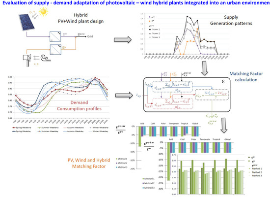
• The evaluation of supply–demand balance adaptation of PV+W hybrid plants
• The hybrid plants are integrated into an urban environment
• The results are applicable on a global scale as we have considered real weather data from hundreds of locations spread all over the world and multiple profiles for the characterisation of the demand.

The main technical challenge arises from our requirement to obtain results applicable on a global scale. With that aim, we have considered only real weather data from hundreds of meteorological stations and multiple electricity load profiles for the characterisation of the demand in different seasons and days. These requirements have obliged the authors to carry out extensive work to obtain and validate the input data and get it homogeneous.

Below in Section 2, we introduce the methodology developed to evaluate and quantify the level of adaptation of generation patterns to demand profiles. In Section 3, we present the results of applying this methodology to a wide number of locations worldwide and carry out a sensitivity analysis of the results. Finally, in Section 4, the conclusions of our study are discussed.

2. Methodology

Our work aims to analyse if the generation patterns of PV+W hybrid facilities match better with the demand profiles than if the facilities were considered separately. We will not determine what would be the absolute coverage of electricity that the facilities could provide to the whole electric demand. This approach is like evaluating to what extent the generation and demand curves have the same “shape”.

We propose the evaluation of the adaptation level by the determination of the matching factor (ε). It will be calculated as the average quadratic error between the electric generation patterns and the demand profiles, previously normalised and particularised for every single location under study, as will be detailed below. In this way, ε would be zero when the adjustment is perfect; it means, when the generation and demand curves have the same shape, and ε would rise to one when the difference becomes higher. The proposed methodology to calculate ε is illustrated in Figure 2.

The calculation starts with the collection of hourly climate data representative of an average year in every single location included in the analysis. The data collected have been pressure p, temperature T, wind speed v and irradiation G. To generalise the results, it is essential to count on climatologic data for multiple locations spread around the Earth. With this data, together with the dimensioning and characterisation of a PV+W hybrid facility, we obtain yearly patterns of the foreseen generation for every type of facility $E_x^{pv}$, $E_x^p$ y $E_x^{pv+w}$.

Second, electricity demand profiles are required. To select the appropriate load profiles to be utilised in the calculation of the matching factor, it is required to quantify to what extent the hybrid facilities’ generation would contribute to the country-level aggregated load. With this aim, first we have done a rough estimation of the amount of electricity that could be generated by hybrid facilities placed in an urban environment (buildings) in a scenario of high penetration, and, second, we have calculated the aggregated demand coverage on hourly basis. The hourly aggregated demand coverage was calculated by using Equation (1):

$$Hourly aggregated demand coverage=\frac{NB \times AB \times CF \times AHIC}{RHAD}$$

(1)

where:

• NB is the number of buildings in the relevant country or region
• $AB$ is the share of available buildings in the relevant country or region, defined as those buildings where the installation of a PV+W hybrid facility would be feasible.
• CF is the capacity factor of the PV+W hybrid facility, defined for one specific period as the electricity generated by the hybrid facility in one hour divided into its installed capacity.
• $AHIC$ is an average PV+W hybrid installed capacity.
• RHAD is the hourly aggregated demand representative for the country or area under analysis.

To have an estimate in different scenarios, the calculation of the hourly aggregated demand coverage was done for two regions (Europe and the United States) and a European country (Spain)

Table 2. Region and country specifics for hourly aggregated demand coverage calculation.

Variable	Spain (SP)	Europe EU28 Countries (EU)	US
NB	10,000,000 [60,61]	130,000,000 [62]	142,500,000 [63,64]
CF	50%
RHAD (MWh)	30,000 [65]	400,000 [66,67]	430,000 [68]

shows the specifics of each region or country considered in the calculations.

Table 3. Hourly aggregated demand coverage.

		AHIC (kW)
		2			5			7.5			10
Country/Region		SP	EU	US	SP	EU	US	SP	EU	US	SP	EU	US
AB (% share out of total)	5.0%	1.7%	1.6%	1.7%	4.2%	4.1%	4.1%	6.3%	6.1%	6.2%	8.3%	8.1%	8.3%
	7.5%	2.5%	2.4%	2.5%	6.3%	6.1%	6.2%	9.4%	9.1%	9.3%	12.5%	12.2%	12.4%
	10.0%	3.3%	3.3%	3.3%	8.3%	8.1%	8.3%	12.5%	12.2%	12.4%	16.7%	16.3%	16.6%
	12.5%	4.2%	4.1%	4.1%	10.4%	10.2%	10.4%	15.6%	15.2%	15.5%	20.8%	20.3%	20.7%
	15.0%	5.0%	4.9%	5.0%	12.5%	12.2%	12.4%	18.8%	18.3%	18.6%	25.0%	24.4%	24.9%

shows the hourly aggregate demand coverage of the hybrid facilities for different values of (i) AHIC and (ii) AB. To obtain conservative values, it was set up 50% of CF and limits of 15% for AB and 10 kW for the AHIC. The results show that shares around 10% of hourly aggregated demand coverage could be reached with moderated values of AB and AHIC. The hourly coverage might reach levels over 20% in more optimistic scenarios.

The level of coverage obtained should be considered in the management of ancillary services and market operations. Based on the above, aggregated load profiles have been selected in the calculation of the matching factor.

The demand evolution presents a high dependency on the climate, the distribution of the working days and the consumer´s habits. One of the objectives of this study is to obtain results applicable globally. Hence, we have utilised multiple profiles to characterise the electricity consumption everywhere. The methodology here proposed includes the determination of 16 different hourly demand curve profiles, as shown in

Table 4. Hourly demand profiles.

Hemisphere	Day	Season
		Spring (S)	Summer (U)	Autumn (A)	Winter (W)
Northern (N)	Weekday (D)	LNSD	LNUD	LNAD	LNWD
	Weekend (E)	LNSE	LNUE	LNAE	LNWE
Southern (S)	Weekday (D)	LSSD	LSUD	LSAD	LSWD
	Weekend (E)	LSSE	LSUE	LSAE	LSWE

, distinguishing between (i) the Northern or Southern hemisphere, (ii) the year season and (iii) weekdays and weekends (bank holidays are included in the weekend day category). Based on the above, the demand profiles used in the calculation for every location will be the eight corresponding to the hemisphere where the location is placed.

As has been discussed before, our methodology is applied to quantify the adaptation degree of the generation to the aggregate demand (i.e., for a country) and not only to local demand where the facility is placed (household, garage, shopping centre, etc.). However, the absolute generation level of every facility, even the aggregation of a high number of them cannot be compared to the global, regional or national demand. We are, therefore, obliged to include in the methodology a mechanism to eliminate the scale effect from ε calculation. The way we propose here is to determine normalised patterns for both generation and demand profiles as follows:

• Both demand profiles and generation patterns are considered on an hourly basis.
• The normalisation period for generation and demand is daily.
• The normalised demand profiles are obtained by dividing each hourly data into the respective daily maximum.
• The individual normalised PV and wind daily generation profiles are obtained by dividing each hourly data into the respective daily maximum.
• Three normalised generation profiles for the hybrid facility are obtained as per the following methods:
  • Method 1: By adding the individual PV and W (wind) normalised profiles:

    $$e_x^{pv+w}=e_x^{pv}+e_x^w$$

    (2)
  • Method 2: By dividing every hourly data into the maximum value of both facilities.

    $$e_x^{pv+w}=\frac{E_x^{pv+w}}{max\left(E_x^{pv},E_x^w\right)}$$

    (3)
  • Method 3: By dividing every hourly data into the daily maximum value of the hybrid facility.

    $$e_x^{pv+w}=\frac{E_x^{pv+w}}{max\left(E_x^{pv+w}\right)}$$

    (4)

These three methods to normalise the values of the hourly hybrid generation profiles do not pretend to have a physical sense by themselves. Our methodology is oriented to find out how the matching factor ε changes when the PV and wind facilities are considered together in a hybrid plant. With this aim, what is relevant to quantify this change is to evaluate it by using the results obtained with the same normalisation method.

Figure 3 shows, as an example, the normalised curves for one day in the period under analysis, where it can be seen:

• The normalised demand hourly profiles for a weekday $l_{x,y,D}$ and for a weekend day $l_{x,y,E}$.
• The normalised generation hourly patterns for the PV facility $e_x^{pv}$ and the wind one $e_x^w$.
• Three hourly generation patterns of the hybrid facility $e_x^{pv+w}$, each one normalised according to the corresponding method.

Once the normalised hourly patterns are determined, ε is calculated for every single location by following the next steps:

• The relevant eight normalised demand profiles are selected according to the site location in the Northern or the Southern hemisphere (Table 4).
• For every annual season, ε is calculated for weekdays (5) and for weekend days (6). The weighted average value is calculated using (7):

  $${\epsilon }_{x,y,D}^i=\frac{{{\displaystyle \sum }}_{n_{x,y}^i}{\left[l_{x,y,D}-e_{x,y}^i\right]}^2}{n_{x,y}^i}$$

  (5)

  $${\epsilon }_{x,y,E}^i=\frac{{{\displaystyle \sum }}_{n_{x,y}^i}{\left[l_{x,y,E}-e_{x,y}^i\right]}^2}{n_{x,y}^i}$$

  (6)

  $${\epsilon }_{x,y}^i=\frac{5{\epsilon }_{x,y,D}^i+2{\epsilon }_{x,y,E}^i}{7}$$

  (7)

  where:
  • ${\epsilon }_{x,y,D}^i$ and ${\epsilon }_{x,y,E}^i$ are the matching factors in weekdays $D$ and weekend days $E,$ respectively, for the facility type $i$, placed at the location $x$, during the season $y$.
  • $n_{x,y}^i$ is the number of hours in the season $y$ at the location $x$.
  • $l_{x,y,D}$ and $l_{x,y,E}$ are the normalised demand profiles in weekdays $D$ and weekend days $E,$ respectively, at the hemisphere where is placed the location $x$, during the season $y$.
  • $e_{x,y}^i$ is the generation pattern for the facility type $i$, placed at the location $x$, during the season $y$.
  • ${\epsilon }_{x,y}^i$ is the matching factor of the generation facility type $i$, placed at the location $x$, during the season $y$.
• Finally, the yearly matching factor for each type of facility and location is obtained by averaging the factors calculated for every season as per (8):

  $${\epsilon }_x^i=\overline{{\epsilon }_{xy}^i}=\frac{{\epsilon }_{x.S}^i+{\epsilon }_{x,U}^i+{\epsilon }_{x,A}^i+{\epsilon }_{x,W}^i}{4}$$

  (8)

2.1. Climatic Data

The climate raw data used in this article has been obtained from the Meteonorm database [69]. This commercial software provides, for an average climatic year, among other variables: hourly data of pressure, temperature, superficial wind speed and solar irradiation incident on an optimally tilted solar panel.

Meteonorm provides weather data everywhere on the planet by means of the interpolation of registered variables in specific points. However, we have only used those locations where the meteorological stations are placed and are logging the climatic variables directly. With this criterion, 844 locations spread over the whole planet were selected.

With the objective to generalise the results of the application of the methodology, the selected locations have been classified following the Köppen–Geiger climatic regions, which divides the Earth into regions according to their weather conditions [70,71]. Figure 4 shows the location of the meteorological stations used in this study and their correspondence with the Köppen–Geiger regions.

2.2. Solar PV and Wind Generation Patterns

To estimate the electricity generation, a PV+W hybrid facility prototype has been designed according to the simplified diagram shown in Figure 5.

The electricity produced by the PV facility placed at the location $x$ is calculated with the following expression, adapted from [73]:

$$E_x^{pv}=G_x·A_{PV}·PR·\eta ·\left[1+\alpha \left(T_x-293\right)\right]$$

(9)

where:

• G_x is the total solar irradiation incident on an optimally tilted solar panel.
• $A_{PV}$ the surface covered by solar panels.
• η is the solar PV panel efficiency.
• $PR$ is the facility performance ratio.
• $\alpha$ is the maximum power temperature coefficient.
• $T_x$ is the ambient temperature (the temperature coefficient should be applied to the difference between the solar panel temperature and the standard value of 293 K. Nevertheless, as the solar temperature is not available, the correction has been applied considering the ambient temperature).

Nowadays there are different technologies used in the manufacturing of solar panels; the most widely used is multi-crystalline silicon cells [74]. For the calculation of the electricity generation, it was selected a commercial solar panel manufactured with multi-crystalline silicon cells and an efficiency η of 15.5%. The rest of the solar panel characteristics are shown in

Table 5. Solar panel characteristics [75].

Characteristic	Value
Manufacturer	Trina Solar
Model	TSM-PC14
Cell type	Si Multicrystalline
Maximum Power (STC conditions)	300 W
Efficiency (η)	15.5%
Dimensions (h × w × d)	1956 × 992 × 40 mm3
Temperature Coefficient of maximum power (α)	−0.41%/K

.

The PV facilities present current PR values in the 60 to 90% range [76,77], therefore, in this study, a mean value of 75% was considered for PR.

The area for solar panels was set up in 23.2 m² because it is a medium size surface suitable to be placed on every roof, pergola, etc. According to the characteristics of the solar panel selected, this area means 12 solar panels giving a power capacity of 3.6 kW.

For the wind facility, a vertical-axis wind turbine generator (VAWT) was selected. These types of wind turbines are more efficient in locations where the wind stream presents both high turbulence and continuous variations in the direction, such as in the urban environment [33,37,41]. The VAWT considered in the calculations has a nameplate power of 3.5 kW, similar to the PV installed capacity. Figure 6 shows the VAWT power curve for standard density (ρ_std = 1.225 kg/cm²).

The electricity produced by the wind facility is calculated according to the following equation (adapted from [79]):

$$E_x^w=\rho ·\frac{P_x}{{\rho }_{std}}·t$$

(10)

where:

• $P$ is the output power from the power curve corresponding with the wind speed incident on the el VAWT (Figure 6).
• $\rho$ is the air density.
• $t$ is the time.

Finally, the electricity produced by the PV+W hybrid facility is:

$$E_x^{pv+w}=E_x^{pv}+E_x^w$$

(11)

The energy produced was calculated for each type of facility (PV, wind and PV+W hybrid) in all locations, obtaining the evolution in an average year with climatic conditions characterised for the variables defined in Section 2.1. Figure 7 shows, as an example, the generation curves of the PV, wind and hybrid facilities in an average month of May at one of the locations considered in this study.

One interesting result of this first step of the calculation is the contribution of the electricity sources, PV and wind, to the total hybrid facility production.

Table 6. PV contribution to the PV+W hybrid-facility generation. (See Figure 4 for climate zone codification).

Climate Zone	n° Stations	$\frac{{\mathit{E}}_{\mathit{x}}^{\mathit{p}\mathit{v}}}{{\mathit{E}}_{\mathit{x}}^{\mathit{p}\mathit{v}+\mathit{w}}}$	Climate Zone	n° Stations	$\frac{{\mathit{E}}_{\mathit{x}}^{\mathit{p}\mathit{v}}}{{\mathit{E}}_{\mathit{x}}^{\mathit{p}\mathit{v}+\mathit{w}}}$
Arid	109	0.89	Tropical	66	0.91
BSh	16	0.90	Af	21	0.89
BSk	46	0.86	Am	8	0.93
BWh	27	0.90	As	4	0.87
BWk	20	0.92	Aw	33	0.92
Cold	188	0.83	Temperate	459	0.84
Dfa	29	0.78	Cfa	192	0.87
Dfb	90	0.83	Cfb	162	0.78
Dfc	40	0.81	Cfc	4	0.68
Dfd	4	0.93	Csa	45	0.85
Dsa	1	1.00	Csb	34	0.87
Dsb	3	0.93	Cwa	17	0.91
Dsc	1	0.82	Cwb	5	0.96
Dwa	10	0.88
Dwb	5	0.88	Polar	32	0.71
Dwc	5	0.95	EF	2	0.33
			ET	30	0.74
Global				854	0.84842

shows the PV Facility contribution to the total generation in the group of different climatic regions. Despite the PV and wind capacity being similar, the contribution of PV is a majority with 84% on average; going from 71% in polar climate zones to 91% in tropical areas. This predominance of PV is justified because the facility locations were not chosen with the criterion of having a relevant wind resource.

2.3. Demand Load Profiles

The demand profiles were defined using real data provided from the commercial companies and distributor and transport system operators detailed in

Table 7. Demand load profiles data source [65,80,81,82,83,84].

Hemisphere	Distributor/Operator	Country
North	Red Eléctrica de España	Spain
	PJM	USA–Northeast
	Midcontinent Independent System Operator	USA–West
	Northwest PowerPool	USA–Northwest
South	National Electricity Coordinator	Chile
	Australian Energy Market Operation	Western Australia

.

From all the sources, real hourly demand curves for the 365 days of 2015 were obtained. Then, to determine the sixteen standard demand profiles used in ε calculation (Table 4), the next steps were followed:

• The curves from every load profile were normalised dividing each hourly data into its respective daily maximum.
• Once normalised, the curves were separated out from the season and from weekday and weekend days.
• It was obtained average normalised curves for both hemispheres.

The normalised demand profiles obtained are shown in Figure 8, Figure 9, Figure 10 and Figure 11.

3. Results

Once the normalised generation patterns and demand profiles have been determined, it is possible to obtain ε by applying Equations (5)–(8). The calculation was made individually for the 844 locations defined in Chapter 2.1 by using a Microsoft VBA macro programme in Excel.

The results, sorted by the Köppen–Geiger climate areas, are shown in

Table 8. ε^pv, ε^w and ε^pv+w for every single individual Köeppen–Geiger climatic regions (See Figure 4 for climate zone codification).

Climate Zone	n° Stations	${\mathit{\epsilon }}_{}^{\mathit{p}\mathit{v}}$	${\mathit{\epsilon }}_{}^{\mathit{w}}$	Method 1			Method 2			Method 3
				${\mathit{e}}_{}^{\mathit{p}\mathit{v}+\mathit{w}}={\mathit{e}}_{}^{\mathit{p}\mathit{v}}+{\mathit{e}}_{}^{\mathit{w}}$			${\mathit{e}}_{}^{\mathit{p}\mathit{v}+\mathit{w}}=\frac{{\mathit{E}}_{}^{\mathit{p}\mathit{v}+\mathit{w}}}{\mathit{m}\mathit{a}\mathit{x}\left({\mathit{E}}_{}^{\mathit{p}\mathit{v}},{\mathit{E}}_{}^{\mathit{w}}\right)}$			${\mathit{e}}_{}^{\mathit{p}\mathit{v}+\mathit{w}}=\frac{{\mathit{E}}_{}^{\mathit{p}\mathit{v}+\mathit{w}}}{\mathit{m}\mathit{a}\mathit{x}\left({\mathit{E}}_{}^{\mathit{p}\mathit{v}+\mathit{w}}\right)}$
				${\mathit{\epsilon }}_{}^{\mathit{p}\mathit{v}+\mathit{w}}$	$\frac{{\mathit{\epsilon }}_{}^{\mathit{p}\mathit{v}+\mathit{w}}}{{\mathit{\epsilon }}_{}^{\mathit{p}\mathit{v}}}$	$\frac{{\mathit{\epsilon }}_{}^{\mathit{p}\mathit{v}+\mathit{w}}}{{\mathit{\epsilon }}_{}^{\mathit{w}}}$	${\mathit{\epsilon }}_{}^{\mathit{p}\mathit{v}+\mathit{w}}$	$\frac{{\mathit{\epsilon }}_{}^{\mathit{p}\mathit{v}+\mathit{w}}}{{\mathit{\epsilon }}_{}^{\mathit{p}\mathit{v}}}$	$\frac{{\mathit{\epsilon }}_{}^{\mathit{p}\mathit{v}+\mathit{w}}}{{\mathit{\epsilon }}_{}^{\mathit{w}}}$	${\mathit{\epsilon }}_{}^{\mathit{p}\mathit{v}+\mathit{w}}$	$\frac{{\mathit{\epsilon }}_{}^{\mathit{p}\mathit{v}+\mathit{w}}}{{\mathit{\epsilon }}_{}^{\mathit{p}\mathit{v}}}$	$\frac{{\mathit{\epsilon }}_{}^{\mathit{p}\mathit{v}+\mathit{w}}}{{\mathit{\epsilon }}_{}^{\mathit{w}}}$
Arid	109	0.46	0.60	0.40	−12%	−33%	0.43	−6%	−28%	0.43	−5%	−27%
BSh	16	0.46	0.59	0.40	−12%	−32%	0.43	−6%	−27%	0.43	−5%	−26%
BSk	46	0.46	0.59	0.39	−14%	−33%	0.42	−8%	−28%	0.43	−6%	−27%
BWh	27	0.45	0.58	0.40	−12%	−31%	0.43	−6%	−26%	0.43	−5%	−25%
BWk	20	0.45	0.65	0.42	−6%	−35%	0.44	−3%	−32%	0.44	−3%	−32%
Cold	188	0.47	0.61	0.40	−6%	−35%	0.42	−9%	−30%	0.43	−8%	−29%
Dfa	29	0.47	0.55	0.37	−20%	−33%	0.41	−12%	−26%	0.42	−11%	−25%
Dfb	90	0.47	0.60	0.39	−16%	−35%	0.42	−10%	−30%	0.43	−8%	−29%
Dfc	40	0.47	0.62	0.40	−16%	−36%	0.42	−11%	−32%	0.43	−10%	−31%
Dfd	4	0.47	0.71	0.46	−4%	−37%	0.47	−2%	−35%	0.47	−1%	−35%
Dsa	1	0.46	0.76	0.46	0%	−40%	0.46	0%	−40%	0.46	0%	−40%
Dsb	3	0.46	0.65	0.42	−9%	−36%	0.44	−4%	−32%	0.45	−3%	−32%
Dsc	1	0.47	0.60	0.37	−20%	−38%	0.41	−13%	−32%	0.41	−11%	−31%
Dwa	10	0.47	0.64	0.42	−10%	−35%	0.44	−6%	−31%	0.44	−5%	−31%
Dwb	5	0.46	0.64	0.41	−11%	-36%	0.44	−6%	−32%	0.44	−5%	−31%
Dwc	5	0.45	0.68	0.43	−5%	−37%	0.44	−2%	−35%	0.45	−2%	−35%
Polar	32	0.47	0.56	0.37	−22%	−34%	0.38	−19%	−31%	0.39	−17%	−30%
EF	2	0.49	0.34	0.26	−48%	−24%	0.25	−49%	−27%	0.26	−48%	−25%
ET	30	0.47	0.57	0.37	−20%	−34%	0.39	−16%	−31%	0.40	−15%	−30%
Temperate	459	0.47	0.61	0.39	−15%	−35%	0.42	−9%	−30%	0.43	−8%	−29%
Cfa	192	0.47	0.60	0.40	−15%	−34%	0.43	−8%	−29%	0.43	−7%	−28%
Cfb	162	0.47	0.59	0.38	−19%	−36%	0.41	−13%	−31%	0.42	−11%	−29%
Cfc	4	0.47	0.54	0.35	−25%	−35%	0.39	−18%	−29%	0.39	−16%	−28%
Csa	45	0.46	0.62	0.41	−11%	−35%	0.43	−7%	−31%	0.43	−6%	−30%
Csb	34	0.46	0.63	0.41	−12%	−36%	0.43	−6%	−32%	0.44	−5%	−31%
Cwa	17	0.46	0.64	0.42	−10%	−35%	0.44	−5%	−31%	0.44	−4%	−30%
Cwb	5	0.45	0.67	0.43	−5%	−36%	0.44	−2%	−34%	0.45	−2%	−33%
Tropical	66	0.46	0.63	0.41	−10%	−34%	0.44	−5%	−30%	0.44	−4%	−29%
Af	21	0.46	0.62	0.41	−11%	−34%	0.43	−6%	−29%	0.44	−5%	−29%
Am	8	0.46	0.64	0.42	−9%	−35%	0.44	−4%	−31%	0.45	−3%	−30%
As	4	0.46	0.55	0.39	−16%	−30%	0.42	−8%	−23%	0.43	−6%	−22%
Aw	33	0.46	0.64	0.42	−9%	−35%	0.44	−5%	−31%	0.44	−4%	−30%
Global	854	0.46	0.60	0.4	−15%	−35%	0.42	−8.9%	−30%	0.43	−7.7%	−29%

.

The global matching factor obtained for PV facilities ${\epsilon }^{PV}$ is 0.46. As it can be noted, this value is quite homogeneous in all the climatic regions.

The global matching factor for the wind facilities ${\epsilon }^W$ is 0.6, that means 30% worse adaptation to demand profiles than PV plants. The results present a low dispersion degree with respect to the climatic areas. The minimum value of 0.56 is obtained for polar climates (−5% out of global value), while the maximum, 0.63, is found for tropical climates (+7% out of global).

For PV+W hybrid plants, depending on the normalisation method, the results obtained for ${\epsilon }^{PV+W}$ go from 0.4 if the method 1 is used, to 0.42 if the method 2 is used and 0.43 if the method 3 is used. Once again, the minimum factor is obtained for sites located in polar climates and the maximum for tropical areas. The degree of dispersion is also very negligible.

Figure 12 illustrates the comparison of the matching factor for the PV+W hybrid plants ${\epsilon }^{PV+W}$ versus PV facilities ${\epsilon }^{PV}$. As it can be noted, in a global context, the adaptation of the hybrid facility is 15% higher for the method 1, 9% higher for the method 2 and 7.7% for the method 3. The highest improvement is given for polar climate areas and the lowest for arid and tropical areas.

The comparison of the matching factor for the PV+W hybrid facility ${\epsilon }^{PV+W}$ versus wind ${\epsilon }^W$ is shown in Figure 13. The adaptation is much higher in this case than when it is compared with the PV facility; as it has obtained an improvement of 35% for the method 1, 30% for the method 2 and 29% for the method 3. The values are quite similar in all the climate areas.

3.1. Sensitivity Analysis

It is mandatory to check if the methodology here proposed would give stable results in case of the variation of the relevant variables considered in the calculations. The technical characteristics of the facilities, as well as the performance parameters of the equipment, are quite steady and will be under control with adequate maintenance. The more relevant variations can arise from (i) deviations or errors in the evaluation of the solar and wind resource at the location or the use of non-optimised facilities (i.e., tilt or azimuth angles of the PV facility different from the ideal) and (ii) different power capacity of the facilities. In this way, to determine the robustness of the methodology two sensitivity analyses were carried out with respect to those variables.

3.1.1. Sensitivity Related to Errors in the Resource Valuation

To evaluate the variations in the valuation of the resource produced by errors, spatial smoothing effector the installation of the facilities (non-optimisation), the electricity generated is calculated by means of a modification of the Formulas (9) and (10) to include the multiplying factors f_pv and f_w to simulate the variation of the solar irradiance and wind resource. The methodology was applied for a wide variation range of the multiplying factors between 0.7 to 1.3 which represents a variation of ±30% in the renewable resources.

$$E_x^{pv}\left(f_{pv}\right)=f_{pv}·G_x·A_{PV}·PR·\eta ·\left[1+\alpha \left(T_x-293\right)\right]$$

(12)

$$E_x^w\left(f_w\right)=\rho ·\frac{P_x\left(f_w\right)}{{\rho }_{std}}·t$$

(13)

The variation of ${\epsilon }^{PV+W}$with the multiplication factors is illustrated in the Figure 14. As it can be shown, the methodology is robust because:

• ${\epsilon }^{PV+W}$ hardly varies with changes of the irradiation for the three normalisation methods.
• The effect of variations in wind resource is quite limited. For increases in the mean wind speed of 30% (f_w = 1.3) ${\epsilon }^{PV+W}$ rises about 5%, while a decrement of 30% (f_w = 0.7) produces a variation range from −5%, (normalisation method 3) to −8% (normalisation method 1).

3.1.2. Sensitivity Related to the Power Capacity of the Facilities

We applied the methodology considering generation patterns of a PV+W hybrid facility with twice the power capacity of the facility previously considered to evaluate the potential variations in the results produced by changes on the installed power capacity of the wind and PV facilities. The solar panel and VAWT used now have the following characteristics:

• A commercial solar panel manufactured with multi-crystalline silicon cells and an efficiency η of 17.5%. The rest of the solar panel characteristics are shown in the

  Table 9. Solar panel characteristics [85].

  Characteristic	Value
  Manufacturer	Trina Solar
  Model	TSM-PD14
  Cell type	Si Multicrystalline
  Maximum Power (STC conditions)	320 W
  Efficiency (η)	17.5%
  Dimensions (h × w × d)	1960 × 992 × 40 mm3
  Temperature Coefficient of maximum power (α)	−0.41%/K

  .

2.

For the wind facility, a vertical-axis wind turbine generator was selected with a nameplate power capacity of 6 kW (similar to the PV facility capacity). Figure 15 shows the VAWT power curve for standard density (ρ_std = 1.225 kg/cm²).

Figure 16 illustrates the comparison of the matching factor for PV+W hybrid plants ${\epsilon }^{PV+W}$ versus PV ${\epsilon }^{PV}$ obtained for facilities with a power capacity of 3.6 kW and 6 kW. In a global context, the adaptation obtained for the 6 kW facility is 19% higher for the method 1, 15% higher for the method 2 and 13% for the method 3. When it is compared with the 3.6 kW, the improvement of the 6 kW facility is higher in all the climate areas.

The matching factor for the PV+W hybrid ${\epsilon }^{PV+W}$ versus wind facilities ${\epsilon }^W$ obtained for the facilities of 3.6 kW and 6 kW is compared in Figure 17. As was obtained for the 3.6 kW facility, the improvement of the matching factor obtained for the 6 kW facility is better when it is compared with the wind facility than when it is compared with the PV facility. The improvement now reaches 32% for method 1, 28% for method 2 and 27% for method 3. The values maintain quite similar ranges in all the climate areas.

The variation of ${\epsilon }^{PV+W}$with the multiplication factors introduced in the Chapter 3.1.1. for the 6 kW PV+W hybrid facility is illustrated in the Figure 18. As it can be shown, for the new capacity the methodology also presents a robust performance because the results hardly vary with changes of the irradiation for the three normalisation methods. Once again, the effect of variations in the wind resource is quite limited.

4. Discussion

In this paper, we have analysed the behaviour of PV+W hybrid facilities placed in urban areas from the point of view of the adaptability of their generation patterns to the aggregate demand profiles. With this aim, we have designed a novel methodology that includes the definition and calculation of the matching factor (ε) to evaluate and quantify the adaptation level. The novelty of our work is based on three main grounds: (i) the evaluation of supply–demand balance adaptation of PV+W hybrid plants, (ii) the integration of the hybrid plants into an urban environment and (iii) the applicability of the results on a global scale.

The analysis of the generation patterns shows that, in a PV+W hybrid plant where the PV and wind facilities have similar installed power capacity, the PV is always the main contributor in the total energy production in all climate conditions, presenting a global value of 84%, varying from 71% in polar areas to 91% in tropical zones. The main reason for this performance is that the facilities are not placed following a criterion of high-wind-resource location which is common in urban areas.

The results show that PV facilities match demand profiles better than wind energy. The global matching factor obtained for PV ${\epsilon }^{PV}$ is 0.46 while for wind ${\epsilon }^W$ is 0.6, which means 30% worse adaptation level. The difference, once again, is homogeneous in all climate conditions.

Likewise, hybrid plants adapt better to the demand than when the facilities are independently evaluated. The hybrid plants present ${\epsilon }^{PV+W}$ in the 0.4 to 0.43 range, depending on the normalisation method used, which means an improvement between 7.7% and 15% in comparison with the adaptation of PV facilities and between 29% and 35% in comparison with wind plants. Once again, the results are homogeneous for all the climate zones.

The proposed methodology has been found robust because the results obtained do not vary substantially with respect to the variation of the solar irradiation or the mean wind speed at the location under study. The methodology also gives comparable results for facilities with different power capacity.

5. Conclusions

An important technical challenge for a massive RES integration is the lack of manageability of the generation to match the demand. A high RES penetration requires the application of measures focused on planning, operation and flexibility of the whole system to respond to the uncertainty and variability in the supply–demand balance in short timescales. These measures present tangible costs to the system.

The results of this study lead us to state that the implementation of PV+W hybrid plants in urban areas would widen the RES integration limits and reduce the cost of high RES penetration because of the improvement of the manageability derived of a better adaptation to the demand profiles.

Additionally, our work gives valuable and quantifiable support to decision-makers to favour RES penetration into the urban environment, which constitutes a perfect example of distributed generation, with the advantages that this type of generation presents for the electric system.

As a result, a massive installation of PV+W hybrid plants would bring benefits for the whole electric system. Therefore, the author’s workgroup of the Department of Electrical, Electronic and Control Engineering [87] propose and recommend the implementation of PV+W hybrid plants.

A massive integration into the urban environment presents financial, technical and regulatory barriers. The adequation of existing buildings could require the evaluation of subsidies to avoid financial constraints that could slow down the integration. Moreover, the facilities integrated into the urban environment will be likely owned by consumers (i.e., particulars or small/medium size companies) that could use part of the generation for self-consumption. This situation will require specific legislation to regulate the energy trading and implement technical requirements to avoid negative impact on the distribution networks.

References

1. United Nations. UN Climate Change Conference Paris 2015. Available online: http://www.un.org/sustainabledevelopment/cop21/ (accessed on 9 July 2016).
2. United Nations Framework Convention on Climate Change. Available online: http://unfccc.int/2860.php (accessed on 5 July 2016).
3. United Nations Treaty Collection. Paris Agreement. Available online: https://treaties.un.org/pages/ViewDetails.aspx?src=TREATY&mtdsg_no=XXVII-7-d&chapter=27&lang=en (accessed on 9 July 2016).
4. The US Department of Energy; Office of Energy Efficiency & Renewable Energy. The U.S. Department of Energy (DOE) SunShot Initiative. Available online: http://energy.gov/eere/sunshot/sunshot-initiative (accessed on 25 June 2016).
5. The US Department of Energy; Office of Energy Efficiency & Renewable Energy. The U.S. Department of Energy (DOE) Wind Program. Available online: http://energy.gov/eere/wind/about-doe-wind-program (accessed on 25 June 2016).
6. European Climate Foundation. Roadmap 2050: A Practical Guide to a Prosperous, Low Carbon Europe; European Climate Foundation: The Hague, The Netherlands, 2010. [Google Scholar]
7. International Renewable Energy Agency. RESOURCE. 2018. Available online: http://resourceirena.irena.org/gateway/dashboard/ (accessed on 22 April 2018).
8. REN21. Renewables 2018 Global Status Report; REN21 Secretariat: Paris, France, 2018; p. 325. [Google Scholar]
9. Philipps, S.P.; Kost, C.; Schlegl, S. Up-to-Date Levelised Cost of Electricity of Photovoltaics; Fraunhofer Institute for Solar Energy Systems ISE: Freiburg, Germany, 2014. [Google Scholar]
10. Energy Technology Systems Analysis Programme; International Renewable Energy Agency. Wind Power. Technology Brief; International Renewable Energy Agency: Abu Dhabi, UAE, 2016; p. 28. [Google Scholar]
11. Lazard. In Levelized Cost of Energy v11; Lazard: New York, NY, USA, 2017; p. 22.
12. Feldman, D.; Margolis, R.; Boff, D. Q4 2016/Q1 2017 Solar Industry Update; U.S. Department of Energy: Oak Ridge, TN, USA, 2017; p. 83.
13. Huld, T.; Jäger Waldau, A.; Ossenbrink, H.; Szabo, S.; Dunlop, E.; Taylor, N. Cost Maps for Unsubsidised Photovoltaic Electricity; JRC 91937 Joint Research Centre of the European Commission: Brussels, Belgium, 2014; p. 22. [Google Scholar]
14. Moné, C.; Hand, M.; Bolinger, M.; Rand, J.; Heimiller, D.; Ho, J. 2015 Cost of Wind Energy Review; NREL/TP-6A20-66861; National Renewable Energy Laboratory: Golden, CO, USA, 2017; p. 115.
15. International Renewable Energy Agency. Renewable Power Generation Costs in 2017; International Renewable Energy Agency: Abu Dhabi, UAE, 2018; p. 160. [Google Scholar]
16. Cayir Ervural, B.; Evren, R.; Delen, D. A multi-objective decision-making approach for sustainable energy investment planning. Renew. Energy 2018, 126, 387–402. [Google Scholar] [CrossRef]
17. Patlitzianas, K.D.; Doukas, H.; Kagiannas, A.G.; Psarras, J. Sustainable energy policy indicators: Review and recommendations. Renew. Energy 2008, 33, 966–973. [Google Scholar] [CrossRef]
18. Liu, G.; Li, M.; Zhou, B.; Chen, Y.; Liao, S. General indicator for techno-economic assessment of renewable energy resources. Energy Convers. Manag. 2018, 156, 416–426. [Google Scholar] [CrossRef]
19. International Energy Agency. IEA Energy Technology Perspectives 2017; International Energy Agency: Paris, France, 2017. [Google Scholar]
20. International Energy Agency. Technology Roadmap Wind Energy. 2013 Edition; International Energy Agency: Paris, France, 2013; p. 63. [Google Scholar]
21. International Energy Agency. Technology Roadmap Solar Photovoltaic Energy. 2014 Edition; International Energy Agency: Paris, France, 2014; p. 20. [Google Scholar]
22. International Renewable Energy Agency. REmap: Roadmap for a Renewable Energy Future; International Renewable Energy Agency: Abu Dhabi, UAE, 2016; p. 172. [Google Scholar]
23. International Renewable Energy Agency. Renewable Energy in Cities; International Renewable Energy Agency: Abu Dhabi, UAE, 2016; p. 64. [Google Scholar]
24. Karteris, M.; Slini, T.; Papadopoulos, A.M. Urban solar energy potential in Greece: A statistical calculation model of suitable built roof areas for photovoltaics. Energy Build. 2013, 62, 459–468. [Google Scholar] [CrossRef]
25. Defaix, P.R.; van Sark, W.G.J.H.M.; Worrell, E.; de Visser, E. Technical potential for photovoltaics on buildings in the EU-27. Sol. Energy 2012, 86, 2644–2653. [Google Scholar] [CrossRef]
26. Singh, R.; Banerjee, R. Estimation of rooftop solar photovoltaic potential of a city. Sol. Energy 2015, 115, 589–602. [Google Scholar] [CrossRef]
27. Wiginton, L.K.; Nguyen, H.T.; Pearce, J.M. Quantifying rooftop solar photovoltaic potential for regional renewable energy policy. Comput. Environ. Urban Syst. 2010, 34, 345–357. [Google Scholar] [CrossRef]
28. Colmenar-Santos, A.; Campíñez-Romero, S.; Pérez-Molina, C.; Mur-Pérez, F. An assessment of photovoltaic potential in shopping centres. Sol. Energy 2016, 135, 662–673. [Google Scholar] [CrossRef]
29. Mohajeri, N.; Upadhyay, G.; Gudmundsson, A.; Assouline, D.; Kämpf, J.; Scartezzini, J.-L. Effects of urban compactness on solar energy potential. Renew. Energy 2016, 93, 469–482. [Google Scholar] [CrossRef] [Green Version]
30. Song, X.; Huang, Y.; Zhao, C.; Liu, Y.; Lu, Y.; Chang, Y.; Yang, J. An Approach for Estimating Solar Photovoltaic Potential Based on Rooftop Retrieval from Remote Sensing Images. Energies 2018, 11, 3172. [Google Scholar] [CrossRef]
31. Polo, M.-E.; Pozo, M.; Quirós, E. Circular Statistics Applied to the Study of the Solar Radiation Potential of Rooftops in a Medium-Sized City. Energies 2018, 11, 2813. [Google Scholar] [CrossRef]
32. Moraitis, P.; Kausika, B.; Nortier, N.; van Sark, W. Urban Environment and Solar PV Performance: The Case of the Netherlands. Energies 2018, 11, 1333. [Google Scholar] [CrossRef]
33. Toja-Silva, F.; Colmenar-Santos, A.; Castro-Gil, M. Urban wind energy exploitation systems: Behaviour under multidirectional flow conditions—Opportunities and challenges. Renew. Sustain. Energy Rev. 2013, 24, 364–378. [Google Scholar] [CrossRef]
34. Araújo, A.M.; de Alencar Valença, D.A.; Asibor, A.I.; Rosas, P.A.C. An approach to simulate wind fields around an urban environment for wind energy application. Environ. Fluid Mech. 2013, 13, 33–50. [Google Scholar] [CrossRef]
35. Grant, A.; Johnstone, C.; Kelly, N. Urban wind energy conversion: The potential of ducted turbines. Renew. Energy 2008, 33, 1157–1163. [Google Scholar] [CrossRef] [Green Version]
36. Grieser, B.; Sunak, Y.; Madlener, R. Economics of small wind turbines in urban settings: An empirical investigation for Germany. Renew. Energy 2015, 78, 334–350. [Google Scholar] [CrossRef]
37. Pagnini, L.C.; Burlando, M.; Repetto, M.P. Experimental power curve of small-size wind turbines in turbulent urban environment. Appl. Energy 2015, 154, 112–121. [Google Scholar] [CrossRef]
38. Alexandru-Mihai, C.; Alexandru, B.; Ionut-Cosmin, O.; Florin, F. New Urban Vertical Axis Wind Turbine Design. INCAS Bull. 2015, 7, 67–76. [Google Scholar] [CrossRef]
39. Carcangiu, S.; Montisci, A. A building-integrated eolic system for the exploitation of wind energy in urban areas. In Proceedings of the 2012 IEEE International Energy Conference and Exhibition (ENERGYCON), Florence, Italy, 9–12 September 2012; pp. 172–177. [Google Scholar]
40. Pagnini, L.; Piccardo, G.; Repetto, M.P. Full scale behavior of a small size vertical axis wind turbine. Renew. Energy 2018, 127, 41–55. [Google Scholar] [CrossRef]
41. Micallef, D.; van Bussel, G. A Review of Urban Wind Energy Research: Aerodynamics and Other Challenges. Energies 2018, 11, 2204. [Google Scholar] [CrossRef]
42. Klima, K.; Apt, J. Geographic smoothing of solar PV: Results from Gujarat. Environ. Res. Lett. 2015, 10, 104001. [Google Scholar] [CrossRef]
43. Monforti, F.; Huld, T.; Bódis, K.; Vitali, L.; D’Isidoro, M.; Lacal Arantegui, R. Assessing complementarity of wind and solar resources for energy production in Italy. A Monte Carlo approach. 2014, 63, 576–586. [Google Scholar] [CrossRef]
44. Santos-Alamillos, F.J.; Pozo-Vázquez, D.; Ruiz-Arias, J.A.; Lara-Fanego, V.; Tovar-Pescador, J. Analysis of Spatiotemporal Balancing between Wind and Solar Energy Resources in the Southern Iberian Peninsula. J. Appl. Meteorol. Climatol. 2012, 51, 2005–2024. [Google Scholar] [CrossRef]
45. Widen, J. Correlations Between Large-Scale Solar and Wind Power in a Future Scenario for Sweden. IEEE Trans. Sustain. Energy 2011, 2, 177–184. [Google Scholar] [CrossRef]
46. Zhang, H.; Cao, Y.; Zhang, Y.; Terzija, V. Quantitative synergy assessment of regional wind-solar energy resources based on MERRA reanalysis data. Appl. Energy 2018, 216, 172–182. [Google Scholar] [CrossRef]
47. Prasad, A.A.; Taylor, R.A.; Kay, M. Assessment of solar and wind resource synergy in Australia. Appl. Energy 2017, 190, 354–367. [Google Scholar] [CrossRef]
48. Huber, M.; Dimkova, D.; Hamacher, T. Integration of wind and solar power in Europe: Assessment of flexibility requirements. Energy 2014, 69, 236–246. [Google Scholar] [CrossRef] [Green Version]
49. Solomon, A.A.; Kammen, D.M.; Callaway, D. Investigating the impact of wind–solar complementarities on energy storage requirement and the corresponding supply reliability criteria. Appl. Energy 2016, 168, 130–145. [Google Scholar] [CrossRef] [Green Version]
50. Jurasz, J.; Beluco, A.; Canales, F.A. The impact of complementarity on power supply reliability of small scale hybrid energy systems. Energy 2018, 161, 737–743. [Google Scholar] [CrossRef]
51. The US Department of Energy, Office of Electricity Delivery & Energy Reliability. The Potential Benefits of Distributed Generation and the Rate-Related Issues That May Impede Its Expansion; U.S. Department of Energy: Oak Ridge, TN, USA, 2015.
52. Abdmouleh, Z.; Gastli, A.; Ben-Brahim, L.; Haouari, M.; Al-Emadi, N.A. Review of optimization techniques applied for the integration of distributed generation from renewable energy sources. Renew. Energy 2017, 113, 266–280. [Google Scholar] [CrossRef]
53. Ruiz-Romero, S.; Colmenar-Santos, A.; Gil-Ortego, R.; Molina-Bonilla, A. Distributed generation: The definitive boost for renewable energy in Spain. Renew. Energy 2013, 53, 354–364. [Google Scholar] [CrossRef]
54. Mai, T.; Wiser, R.; Sandor, D.; Brinkman, G.; Heath, G.; Denholm, P.; Hostick, D.J.; Darghouth, N.; Schlosser, A.; Strzepek, K. Exploration of High-Penetration Renewable Electricity Futures; NREL/TP-6A20-52409-1; National Renewable Energy Laboratory: Golden, CO, USA, 2012.
55. International Energy Agency. System Integration of Renewables. An update on Best Practice; International Energy Agency: Paris, France, 2018. [Google Scholar]
56. Batalla-Bejerano, J.; Trujillo-Baute, E. Impacts of intermittent renewable generation on electricity system costs. Energy Policy 2016, 94, 411–420. [Google Scholar] [CrossRef]
57. Delarue, E.; Van Hertem, D.; Bruninx, K.; Ergun, H.; May, K.; Van den Bergh, K. Determining the Impact of Renewable Energy on Balancing Costs, Back Up Costs, Grid Costs and Subsidies; Report for Adviesraad Gas en Elektriciteit—CREG; CREG: Brussels, Belgium, 2016. [Google Scholar]
58. Hirth, L.; Ueckerdt, F.; Edenhofer, O. Integration costs revisited—An economic framework for wind and solar variability. Renew. Energy 2015, 74, 925–939. [Google Scholar] [CrossRef]
59. Shang, Y. Resilient Multiscale Coordination Control against Adversarial Nodes. Energies 2018, 11, 1844. [Google Scholar] [CrossRef]
60. Spanish National Statistics Centre. Buildings and Population Census; Spanish National Statistics Centre: Madrid, Spain, 2019. [Google Scholar]
61. Spanish Ministry of Development. Buildings Construction Licences; Spanish Ministry of Development: Madrid, Spain, 2019. [Google Scholar]
62. Eurostat. CensusHub2. 2019. Available online: https://ec.europa.eu/CensusHub2/query.do?step=selectHyperCube&qhc=false (accessed on 20 March 2019).
63. U.S. Census Bureau. American FactFinder. Annual Estimates of Housing Units for the United States, Regions, Divisions, States, and Counties: April 1, 2010 to July 1, 2017. 2017 Population Estimates. Available online: https://factfinder.census.gov/faces/tableservices/jsf/pages/productview.xhtml?pid=PEP_2018_PEPANNRES&src=pt (accessed on 20 March 2019).
64. U.S. Energy Information Administration. Commercial Buildings Energy Consumption Survey (CBECS); U.S. Energy Information Administration: Washington, DC, USA, 2016.
65. Red Eléctrica de España, S.A. Esios. System Operator Information System. Available online: https://www.esios.ree.es/en/analysis/10004?vis=1&start_date=31-03-2016T00%3A00&end_date=31-03-2016T23%3A50&compare_start_date=30-03-2016T00%3A00&groupby=minutes10&compare_indicators=545,544 (accessed on 2 April 2018).
66. ENTSO-E. Electricity in Europe 2017. Synthetic Overview of Electric System Consumption, Generation and Exchanges in 34 European Countries; ENTSO-E: Brussels, Belgium, 2018; p. 20. [Google Scholar]
67. ENTSO-E. Monthly Hourly Load Values; ENTSO-E: Brussels, Belgium, 2019. [Google Scholar]
68. U.S. Energy Information Administration. U.S. Electric System Operating Data; U.S. Energy Information Administration: Washington, DC, USA, 2019.
69. Meteotest Genossenchaff Meteonorm, 7th ed. Available online: https://meteonorm.com/t (accessed on 10 January 2018).
70. Köppen, W.; Geiger, R. Das geographische System der Klimate. In Handbuch der Klimatologie; Köppen, W., Geiger, R., Eds.; Verlag von Gebrüder Borntraeger: Berlin, Germany, 1936; Volume I, p. 44. [Google Scholar]
71. Kottek, M.; Grieser, J.; Beck, C.; Rudolf, B.; Rubel, F. World Map of the Köppen-Geiger climate classification updated. Meteorol. Z. 2006, 15, 259–263. [Google Scholar] [CrossRef]
72. University of Veterinary Medicine Vienna. Institute for Veterinary Public Health. World Maps of Köppen-Geiger Climate Classification. Available online: http://koeppen-geiger.vu-wien.ac.at/ (accessed on 20 June 2016).
73. Duffie, J.A.; Beckman, W.A.; Worek, W.M. Solar Engineering of Thermal Processes, 4th ed.; John Wiley & Sons, Inc.: Hoboken, NJ, USA, 2013; p. 928. [Google Scholar]
74. International Technology Roadmap for Photovoltaic. ITRPV 2017 Results; VDMA: Francfurt, Germany, 2018; p. 71. [Google Scholar]
75. Trina Solar. Products. PC14. 72-Cell Utility Module. Available online: http://www.trinasolar.com/uk/product/PC14.html (accessed on 15 May 2016).
76. Reich, N.H.; Mueller, B.; Armbruster, A.; van Sark, W.G.J.H.M.; Kiefer, K.; Reise, C. Performance ratio revisited: Is PR > 90% realistic? Prog. Photovolt. Res. Appl. 2012, 20, 717–726. [Google Scholar] [CrossRef]
77. Dierauf, T.; Growitz, A.; Kurtz, S.; Becerra Cruz, J.L.; Riley, E.; Hansen, C. Weather-Corrected Performance Ratio; NREL/TP-5200-57991; National Renewable Energy Laboratory: Golden, CO, USA, 2013.
78. V-AIR. Vertical Axis Wind Turbine VisionAir5. Available online: http://www.visionairwind.com/wp-content/uploads/2018/08/VisionAIR5.pdf (accessed on 6 April 2019).
79. Carta González, J.A.; Calero Pérez, R.; Colmenar-Santos, A.; Castro Gil, M.-A. Centrales de Energías Renovables: Generación Eléctrica con Energías Renovables; Pearson Educación, S.A.: Madrid, Spain, 2009; p. 728. [Google Scholar]
80. PJM. Data Viewer. Load. Available online: https://dataviewer.pjm.com/dataviewer/pages/public/load.jsf (accessed on 2 April 2018).
81. Northwest Power Pool. Geographic NWPP Aggregated Wind Generation and Load Data. Available online: http://www.nwpp.org/our-resources/NWPP-Reserve-Sharing-Group/Geographic-NWPP-Aggregated-Wind-Generation-and-Load-Data (accessed on 2 April 2018).
82. Midcontinent Independent System Operator. I. Market Reports. Available online: https://www.misoenergy.org/markets-and-operations/market-reports/#nt=%2FMarketReportType%3ASummary%2FMarketReportName%3ADaily%20Regional%20Forecast%20and%20Actual%20Load%20(xls)&t=10&p=0&s=MarketReportPublished&sd=desc (accessed on 2 April 2018).
83. Coordinador Eléctrico Nacional. Operación Real. Available online: https://sic.coordinador.cl/informes-y-documentos/fichas/operacion-real/ (accessed on 1 April 2018).
84. Australian Energy Market Operation. Electricity Load Profiles—Aggregated Price and Demand Data—Historical. Available online: https://www.aemo.com.au/Electricity/National-Electricity-Market-NEM/Data-dashboard#aggregated-data (accessed on 1 April 2018).
85. Trina Solar. Products. PD14. 72-Cell Utility Module. Available online: http://static.trinasolar.com/sites/default/files/ES_TSM_PD14_datasheet_B_2017_web.pdf (accessed on 21 April 2018).
86. Kingspan Renewable Technologies. KW6 Wind Turbine. Available online: https://www.kingspan.com/gb/en-gb/products/renewable-technologies/wind-energy/kw6-wind-turbine (accessed on 21 April 2018).
87. National Distance Education University. Department of Electrical, Electronic and Control Engineering. Available online: http://www2.uned.es/personal/antoniocolmenar/publicaciones.htm (accessed on 1 May 2016).
Figure 1. Wind and photovoltaic (PV) installed power worldwide. Source: [7,8].
Energies 12 01780 g001
Figure 2. Methodology for obtaining the matching factor (ε) at a single location.
Energies 12 01780 g002
Figure 3. One-day-example of the normalised generation and load profile evolution.
Energies 12 01780 g003
Figure 4. Location of the meteorological stations in the Köppen–Geiger climate classification areas. Source: [72] and self-elaboration.
Energies 12 01780 g004
Figure 5. Single line diagram of the photovoltaic+wind hybrid (PV+W hybrid) facility.
Energies 12 01780 g005
Figure 6. Vertical-axis wind turbine generator (VAWT) power curve for the standard air density ρstd = 1.225 kg/cm2. Source [78].
Energies 12 01780 g006
Figure 7. Time evolution of the generation in May.
Energies 12 01780 g007
Figure 8. Standard normalised demand profiles for weekend days in the Northern Hemisphere. Source: [65,80,81,82] and self-elaboration.
Energies 12 01780 g008
Figure 9. Standard normalised demand profiles for weekdays in the Northern Hemisphere. Source: [65,80,81,82] and self-elaboration.
Energies 12 01780 g009
Figure 10. Standard normalised demand profiles for weekend days in the Southern Hemisphere. Source: [83,84] and self-elaboration.
Energies 12 01780 g010
Figure 11. Standard normalised demand profiles for weekdays in the Southern Hemisphere. Source: [83,84] and self-elaboration.
Energies 12 01780 g011
Figure 12. Improvement of the matching factor: εpv+w (hybrid) over εpv (solar PV) facilities.
Energies 12 01780 g012
Figure 13. Improvement of the matching factor: εpv+w (hybrid) over εw (wind) facilities.
Energies 12 01780 g013
Figure 14. Variation of ε P V + W with the multiplication factors fpv and fw. (M1, M2 and M3 represent the results obtained by means of application of the normalisation methods 1, 2 and 3, respectively).
Energies 12 01780 g014
Figure 15. Power curve for the standard air density ρstd = 1.225 kg/cm2. Source [86].
Energies 12 01780 g015
Figure 16. Improvement of the matching factor: εpv+w (hybrid) over εpv (PV) facilities for different installed power capacity.
Energies 12 01780 g016
Figure 17. Improvement of the matching factor: εpv+w (hybrid) over εw (wind) facilities for different installed power capacity.
Energies 12 01780 g017
Figure 18. Variation of ε P V + W with the multiplication factors fpv and fw. in a 6 kW power capacity facility (M1, M2 and M3 represent the results obtained by means of application of the normalisation methods 1, 2 and 3, respectively).
Energies 12 01780 g018