Optimal Sizing of Photovoltaic Generation in Radial Distribution Systems Using Lagrange Multipliers

Abstract

The integration of renewable distributed generation into distribution systems has been studied comprehensively, due to the potential benefits, such as the reduction of energy losses and mitigation of the environmental impacts resulting from power generation. The problem of minimizing energy losses in distribution systems and the methods used for optimal integration of the renewable distributed generation have been the subject of recent studies. The present study proposes an analytical method which addresses the problem of sizing the nominal power of photovoltaic generation, connected to the nodes of a radial distribution feeder. The goal of this method is to minimize the total energy losses during the daily insolation period, with an optimization constraint consisting in the energy flow in the slack bus, conditioned to the energetic independence of the feeder. The sizing is achieved from the photovoltaic generation capacity and load factors, calculated in time intervals defined in the typical production curve of a photovoltaic unit connected to the distribution system. The analytical method has its foundations on Lagrange multipliers and relies on the Gauss-Jacobi method to make the resulting equation system solution feasible. This optimization method was evaluated on the IEEE 37-bus test system, from which the scenarios of generation integration were considered. The obtained results display the optimal sizing as well as the energy losses related to additional power and the location of the photovoltaic generation in distributed generation integration scenarios.

1. Introduction

The smart grid concept has as premise the stimulus of the adoption of more efficient technologies which should contribute to the reduction of technical losses and the mitigation of negative environmental impacts derived from the operation of the current electrical system [1], for example, greenhouse gas emission (GGE) mitigation, for the energy input in the distribution system. In this context, distributed generation (DG) plays a leading role in boosting the adoption of renewable energy sources in the system, such as photovoltaic generation (PV). The inherent relations between DG and smart grids, in addition to the roles of consumers in demand response mechanisms, have become the theme of discussions and scientific research [2]. It is important to highlight that when accounting for the energy losses, environmental impacts related to distribution systems cannot be neglected, since they contribute to total GGE, adding to the electric power generation and transmission segments [3]. From this perspective, when traditional distribution system planning adopts strategies to integrate DG, the analysis of efficiency and quality aspects, such as meeting voltage levels and loading limit standards, as well as power flow and grid losses analyses, must be expanded. In addition, in order to achieve a higher level of benefits from the integration of DG into the power grid, proper optimization techniques must be applied in order to better size the generation, handling problems that may contain multiple objectives and present specific constraints.

The topic of optimum dispatch in transmission systems has been discussed since the 1960s, as in [4], where Lagrange multipliers were used for the calculation of the optimal generated power division, based on the incremental cost principle. However, only an approximate calculation for transmission system losses was made, a measure which is well known to influence the results. A similar analysis was carried out in [5], using the Lagrange method applied to economic generation programming. In that study losses calculations were obtained by applying an equation for the bus impedance matrix (Z_bus), which relates losses to the net power input in each bus. The same problem was approached in [6], aiming to optimize losses by minimizing the power provided by the slack bus. The use of methods based on Z_bus in distribution systems, although possible, displays characteristics which can hinder the process. In these systems, the bus admittance matrix (Y_bus) is usually singular, which makes it impossible to obtain the Z_bus matrix through its inversion. On the other hand, obtaining the Z_bus matrix by using a direct algorithm is computationally costly. The gradient method, using constant pitch and applying the Newton-Raphson method, by calculating the Hessian matrix, was used in [7], where the Lagrange method was also used for the iterative solution of the optimal generation resource sizing problem. However, the fact that the Hessian matrix is singular in a larger distribution network is an obstacle for the application of this method.

The methods used for the optimal integration of renewable DG in distribution networks have been critically reviewed in recent articles. In [8], the authors review conventional techniques and metaheuristic algorithms for optimal DG planning in distribution networks, while also reviewing and performing a comparative analysis of the analytical techniques used for optimal DG integration. Motivators and challenges for DG increase are addressed in [9], as well as a general review of optimization methods used for DG planning and integration, focusing on optimum DG allocation and sizing. A taxonomic revision of DG planning in distribution systems is presented in [10], based on a comprehensive comparative performance classification for several IEEE test systems, artificial intelligence computational techniques, conventional optimization techniques for optimal DG planning in distribution networks, from several papers. A comprehensive review of DG allocation was carried out in [11], from the viewpoint of classification and comparison of several objective functions and their constraints, aiming to minimize power or total energy losses, improving the voltage profile and financial optimization for DG penetration. The authors of [11] also compare applied methods and optimization algorithms, such as classical approaches, basic research methods, algorithms inspired by physics or social relationships, nature-inspired techniques and hybrid intelligent algorithms.

Thus, the optimal allocation and sizing problem for renewable DG has been continuously studied. Several different approaches have been applied to minimize total energy power losses in distribution networks. Many studies discussing the optimal dispatch for distribution system problems use metaheuristics such as algorithm and as an approach technique. A genetic algorithm is used in [12] for optimal DG allocation and sizing; in [13], for optimal location and sizing of distributed PV generations, with battery storage systems; in [14], it is applied to a fuzzy-based model, to approach the uncertainty and load variability problem. The stochastic nature of the PV generation penetration problem is also treated in [15], which proposes a stochastic power flow and a solution from a probabilistic model. Other metaheuristics, such as the artificial bee colony algorithm [16,17], the particle swarm optimization [18,19] and the grey wolf optimizer [20] methods, as well as the ant lion optimizer [21] algorithm, are currently used for optimal DG sizing, aiming to minimize distribution network losses. However, the metaheuristics demand the performance of a high number of load flow calculations with the aim of providing satisfactory results for a problem, with no guarantee of optimality.

Analytical methods also have been proposed for the renewable DG integration problem. In [22], the Newton-Raphson numerical method is used to solve the non-linear system of the problem, which comprises generator integration with the objective of reducing both energy losses and generation costs. Initially, the study searches for the generator installation site through a simplified full-mixed programming model and uses a numeric method for generation sizing. In [23], an analytical method is proposed, in which a power flow for optimal sizing and allocation of several DG types is used to minimize losses by the calculation of the partial differentials of active losses. In [24], the analytical method aims to minimize the losses associated to the active and reactive components of the current inputted by the DG.

In this context, the present study proposes an analytical method that addresses the problem of the sizing of nominal powers of multiple PV generation units connected to a radial distribution feeder, in order to minimize total energy losses during the daily insolation period. This sizing is defined considering the typical production curve for a PV unit connected to the system and the typical distribution feeder load curve. From these curves, the proposed method uses a PV generation capacity and load factors, calculated in time intervals defined by daily insolation periods. Thus, the proposed methodology examines the energy losses throughout the entire cycle of the curve, not only minimizing total power losses at a load or PV generation demand peak. The analytical method was evaluated based on Lagrange multipliers and an iterative algorithm was developed using the Gauss-Jacobi method. Therefore, the highlights of this study are:

• The application of Lagrange multiplier optimization along with the Gauss-Jacobi method to obtain a feasible solution.
• The assembly of the optimization problem by using the Lagrange augmented objective function, combined with a tree gradient calculation [25] for radial distribution systems.
• The determination of generator optimal nominal power considering a variable PV generation capacity and load factors during the insolation period.
• The proposed optimization method is based on gradients, with higher convergence rate—by not using the arbitrary step (gradient method)—and less computational effort, since it does not use the Hessian matrix (Newton’s method).
• The use of an energy balance limit as a constraint for the problem, minimizing the slack bus flow and leading to the energetic feeder independence.

This study has the following structure: Section 2 presents the approach to the PV generation integration problem and distribution system energy losses balancing; Section 3 contains the proposed methodology and the procedures to solve the problem; Section 4 presents the evaluation of the method using an IEEE 37-bus test system and presents and discusses the simulation numerical results; and Section 5 discusses the conclusions of the study.

2. Problem Approach

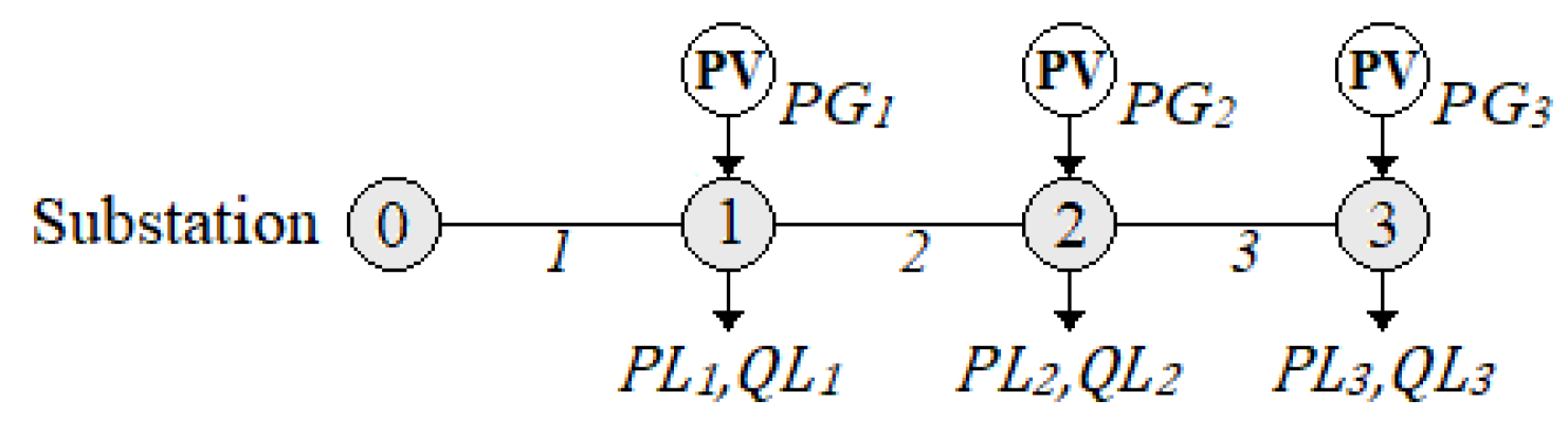
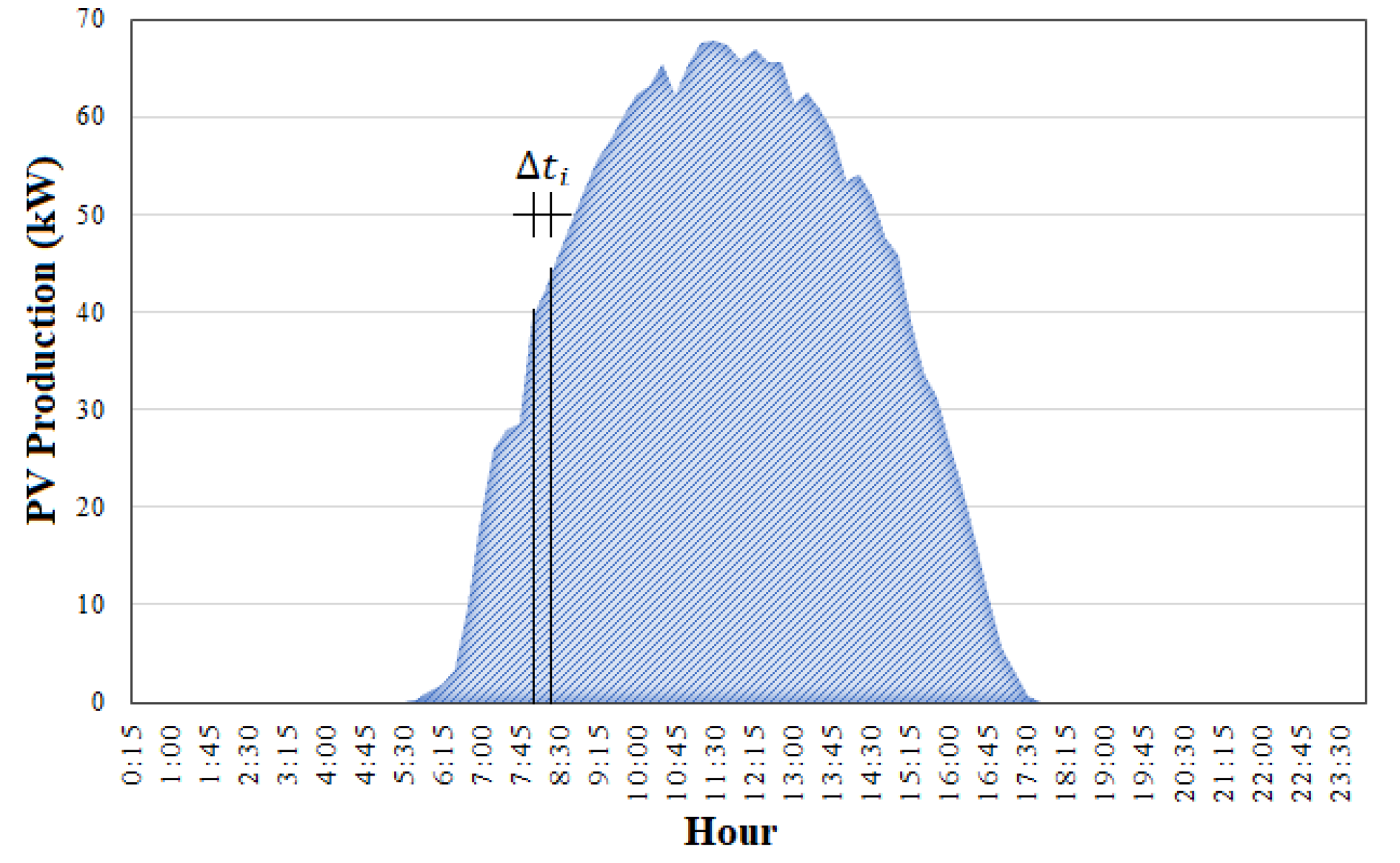
2.1. Photovoltaic Generation Integration

The photovoltaic (PV) generation integration problem in distribution system has been addressed in some countries by regulations. Concerning Brazil, the Normative Resolution from the Brazilian Electricity Regulatory Agency—ANEEL, according to [26], establishes the general conditions for accessing the distributed generation of electrical power, and limits the installed generation power to that made available to the consuming unit where the DG will be connected. In this way, the available power, which the distributor electrical system must provide to consumers is a constraint to the nominal generation power problem installed by the prosumer, given as:

$$P_{DGNk}\le rt·P_{Ak},$$

(1)

where P_DGNk is the DG k-th nominal power and P_Ak is the power which the distributor should provide to the k-th load bus. The ratio limit, rt, determines the DG power from the limits for the relation between P_DGNk and P_Ak for the consuming unit. In the Brazilian resolution, this relation is equal to 1.0.

PV generation capacity is commonly used in the DG integration problem as the ratio between the electrical power generated in kWh and the nominal kWh generation capacity. To determine the optimal nominal generator power, a generation factor variable throughout the insolation period was considered. The hourly PV generation capacity factor was calculated for each Δt_i, time interval from a daily production curve, Figure 1, of a real PV system connected to a local distribution feeder:

$$C{F}_i=\frac{\Delta P{G}_k}{P_{DGNk}},$$

(2)

where CF_i is the PV generation factor calculated for the i-th Δt_i time interval; ΔPG_k is the mean value for the active power inputted by the k-th PV generator, calculated from the discrete area defined by the Δt_i interval; P_DGNk is the k-th PV generator during the total insolation period; and Δt_i is the time frame of a total insulation period fraction, as displayed in Figure 1. The typical daily production curve adopted comes from the PV generation system connected to the distribution feeder located in Northeastern Brazil.

2.2. Load Modeling

Depending on voltage variations, loads can be classified as constant power or constant impedance loads in distribution system modelling [27]. In the first case, the power consumed by the load is constant, regardless of the voltage at the bus. In the second case, the consumed power varies with the squared value of the voltage. On a typical operation scenario, the distribution network nodes present voltages that are lower than the system’s nominal voltage. This way, the voltage dependent loads require, from the network, powers that are lower than their nominal power. However, on scenarios with lower voltages, the constant power loads require higher loading from the distribution network. The appropriate representation of the load has a direct effect on the load flow results, whereby constant power modelling being the most critical representation, regarding to voltage drops. For this reason, it was adopted for this study.

A variable load factor calculated during the insolation period, was considered for load modelling, in order to evaluate the constant power load values in each one of the distribution system buses. Therefore, the feeder’s typical load curve and production curve are taken in account, Figure 1, with the demand value being observed in each time interval, throughout the whole insolation period. In this way, the load factor is defined as the ratio between the average demand in each interval and the distribution feeder’s peak demand, observed in each Δt_i interval throughout the insolation period, as follows:

$$L{F}_i=\frac{\Delta D_i}{D_{max}},$$

(3)

where LF_i is the feeder’s load factor calculated in the i-th Δt_i interval of the insolation period; ΔD_i is the feeder’s average demand calculated in the i-th Δt_i interval for the time period; and D_max is the feeder’s peak distribution demand for the insolation period.

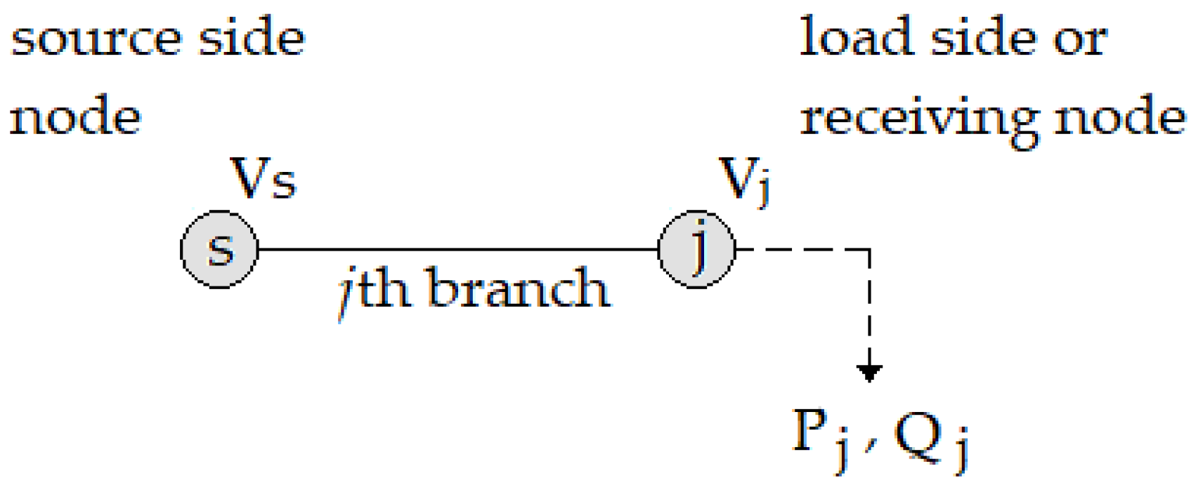
2.3. Energy Losses in Distribution Systems

The losses of total active power for a radial distribution feeder is calculated as the sum of each transmission line stretch active power losses, by:

$$P_{loss}={{\displaystyle \sum }}_{j=1}^{NB}\left(L{P}_j\right),$$

(4)

in which, NB is the total branches and LP_j is the active power loss in the j-th branch. The definitions suggested in [27] are adopted, where the branch number j is the same as the final node j connected to the branch, for j = 1, 2, …, NB.

The active power loss in each branch can be calculated as in [27,28], though:

$$L{P}_j=\frac{R_j\left(P_j{}^2+Q_j{}^2\right)}{V_j^2},$$

(5)

where R_j is the resistance in the j branch e V_j is the voltage magnitude in the j-th node.

The P_j and Q_j terms are, respectively, the sum of the active and reactive power, calculated according to the network elements and components connected downstream to the j node, as defined in:

$$P_j={\displaystyle \sum }PG+{\displaystyle \sum }PL+{\displaystyle \sum }LP,$$

(6)

$$Q_j={\displaystyle \sum }Qcap+{\displaystyle \sum }QL+{\displaystyle \sum }LQ,$$

(7)

where ${\displaystyle \sum }PG$ is the inputted PV generator power sum; ${\displaystyle \sum }Qcap$ is the input capacitor bank power sum; ${\displaystyle \sum }PL$ and ${\displaystyle \sum }QL$ are the sum of active and reactive loads at constant power; and ${\displaystyle \sum }LP$ and ${\displaystyle \sum }LQ$ are the sum of active and reactive power losses in the transmission lines.

The following signal convention must be adopted in (6) and (7), concerning the injected powers and the powers consumed by the loads and in the form of line losses: :

• ${\displaystyle \sum }PG$, ${\displaystyle \sum }{Q}_{cap}$ (injected power): terms must be included in the sum as positive values;
• ${\displaystyle \sum }PL$,${\displaystyle \sum }QL$ (rower consumed by the loads): terms must be included in the sum as negative values;
• ${\displaystyle \sum }LP$,${\displaystyle \sum }LQ$ (power consumed in the form of line losses): terms must be included in the sum as negative values.

The convention adopted above is used, throughout the development of the method proposed, for the input of injected power and consumed power data.

From the equivalent system presented in Figure 2, and according to development in [27], the voltage magnitude in the j-th node, V_j, is calculated from the bi-squared equation, which relates the known voltage in the source side node, s, with the voltage in the load side node, or receiving node, j, as in (8):

$$V_j^4+\left[2\left(R_j{P}_j+X_j{Q}_j\right)-V_s^2\right]V_j^2+\left(R_j^2+X_j^2\right)\left(P_j{}^2+Q_j{}^2\right)=0,$$

(8)

where R_j and X_j are, respectively, the resistance and reactance of the j branch and vs. is the known voltage magnitude at the s-th node. The deduction of the bi-squared Equation (8), is presented in the Appendix A, in accordance with [27].

The total active power losses can be rewritten from (4) and (5) as:

$$P_{loss}={{\displaystyle \sum }}_{j=1}^{NB}\frac{R_j\left(P_j{}^2+Q_j{}^2\right)}{V_j^2}.$$

(9)

The total energy losses (E_loss) is defined in this study as the sum of the total active power losses product by each Δt_i interval, in NI time intervals and is presented as:

$$E_{loss}={{\displaystyle \sum }}_{i=1}^{NI}{P}_{loss}{}_i\Delta t_i,$$

(10)

where i is the insolation interval position NI is the total of time intervals in an insolation period defined in Figure 1, for i = 1, 2, …, NI.

Replacing (4) in (10), the distribution feeder energy losses is calculated as:

$$E_{loss}={{\displaystyle \sum }}_{i=1}^{NI}\left[\Delta t_i{{\displaystyle \sum }}_{j=1}^{NB}\left(L{P}_j\right)\right].$$

(11)

3. Proposed Methodology

The proposed optimization method is structured around the calculation of the gradient vector of the energy losses, E_loss in relation to the nominal powers of the generators, P_DGNk, according to the tree gradient formulation for radial feeders developed in [25]. In addition, the method uses Lagrange multipliers as the optimization technique [29], based on the augmented objective function, the Lagrangian function, and its solution is achieved by the iterative Gauss-Jacobi method. The analytical approach proposed herein presents a better convergence rate guarantee as it does not used arbitrary steps, as in the gradient method presented in [25]. Furthermore, it requires low computational effort, since it does not assemble the Hessian matrix, as, e.g., by Newton’s method.

3.1. Gradient of Total Power Losses

The gradient vector is obtained by differentiating total power losses, from (9), with respect to the nominal power of the k-th generator connected to the distribution feeder, P_DGNk, defined as the control variables of the problem. Adopting the chain rule, the gradients, $\frac{\partial P_{loss}}{\partial P_{DGNk}}$ can be decomposed in terms of the effectively generated power in the k-th generator, PG_k, as:

$$\frac{\partial P_{loss}}{\partial P_{DGNk}}=\frac{\partial P_{loss}}{\partial P{G}_k}·\frac{\partial P{G}_k}{\partial P_{DGNk}}.$$

(12)

For calculation purposes, the second term of the decomposition, $\frac{\partial P{G}_k}{\partial P_{DGNk}}$, is treated as:

$$\frac{\partial P{G}_k}{\partial P_{DGNk}}=\frac{\Delta P{G}_k}{P_{DGNk}}=C{F}_i.$$

(13)

where the generation capacity factor calculation, CF_i, was defined in (2), and is calculated for each PV generator, as a discrete factor in time, from the area defined for each Δt_i interval in Figure 1. Regarding the CF_i calculation, the maximum power value produced by generator PV, during the insolation period presented in the curve displayed in Figure 1, is used as a replacement for P_DGNk.

Isolating the partial derivative of the total power losses in relation to the power generated by the k-th connected generator, $\frac{\partial P_{loss}}{\partial P{G}_k}$, the first term, presented in (12), based on (6), (7) and (9), the following expression is obtained:

$$\frac{\partial P_{loss}}{\partial P{G}_k}={{\displaystyle \sum }}_{j=1}^{NB}\frac{R_j\left(\begin{array}{c}2P_j\left(f_{jk}+{{\displaystyle \sum }}_{m=1}^{NBd}\left(\frac{\partial L{P}_m}{\partial P{G}_k}\right)\right)+\\ 2Q_j\left({{\displaystyle \sum }}_{m=1}^{NBd}\left(\frac{\partial L{Q}_m}{\partial P{G}_k}\right)\right)\end{array}\right)V_j^2}{V_j^4}-{{\displaystyle \sum }}_{j=1}^{NB}\frac{\left(P_j{}^2+Q_j{}^2\right)\frac{\partial V_j^2}{\partial P{G}_k}}{V_j^4},$$

(14)

where NBd is the number of branches connected downstream to the j bus; and factor $f_{jk}$ equals 1, if the k bus is located downstream to the j bus; when this does not occur, it equals 0.

To calculate the derivative $\frac{\partial P_{loss}}{\partial P{G}_k}$, the term $\frac{\partial V_j^2}{\partial P{G}_k}$ should be known. Thus, isolating $V_j^2$ from (8), the following expression is obtained:

$$\begin{gathered} V_j^2=\frac{1}{2}\left\{-\left[2\left(R_j{P}_j+X_j{Q}_j\right)-V_s^2\right]+ \\ \sqrt{{\left[2\left(R_j{P}_j+X_j{Q}_j\right)-V_s^2\right]}^2-4\left(R_j^2+X_j^2\right)\left(P_j{}^2+Q_j{}^2\right)}\right\}. \end{gathered}$$

(15)

Calculating the partial derivative of $V_j^2$ in relation to PG_k, the following expression is defined:

$$\begin{gathered} \frac{\partial V_j^2}{\partial P{G}_k}=\frac{1}{2}\{-2\left(R_j\frac{\partial P_j}{\partial P{G}_k}+X_j\frac{\partial Q_j}{\partial P{G}_k}\right)+\frac{\partial V_s^2}{\partial P{G}_k}+\frac{1}{2}{\left(B^2-4C\right)}^{-\frac{1}{2}}\left[2B\left(2R_j\frac{\partial P_j}{\partial P{G}_k}+2X_j\frac{\partial Q_j}{\partial P{G}_k}-\frac{\partial V_s^2}{\partial P{G}_k}\right)- \\ 8\left(R_j^2+X_j^2\right)\left(P_j\frac{\partial P_j}{\partial P{G}_k}+Q_j\frac{\partial Q_j}{\partial P{G}_k}\right)\right]\}, \end{gathered}$$

(16)

where $B=\left[2\left(R_j{P}_j+X_j{Q}_j\right)-V_s^2\right]$ e $C=\left(R_j^2+X_j^2\right)\left(P_j{}^2+Q_j{}^2\right)$.

Considering that ${{\displaystyle \sum }}_{m=1}^{NBd}\frac{\partial P{L}_m}{\partial P{G}_k}=0$, ${{\displaystyle \sum }}_{m=1}^{NBd}\frac{\partial Q{L}_m}{\partial P{G}_k}=0$ and ${{\displaystyle \sum }}_{m=1}^{NBd}\frac{\partial Qca{p}_m}{\partial P{G}_k}=0$, due to the adoption of constant power loads in the distribution system modelling, the terms $\frac{\partial P_j}{\partial P{G}_k}$ and $\frac{\partial Q_j}{\partial P{G}_k}$, are explicitly determined as: $\frac{\partial P_j}{\partial P{G}_k}={{\displaystyle \sum }}_{m=1}^{NBd}\frac{\partial P{G}_m}{\partial P{G}_k}+{{\displaystyle \sum }}_{m=1}^{NBd}\frac{\partial L{P}_m}{\partial P{G}_k}$ and $\frac{\partial Q_j}{\partial P{G}_k}={{\displaystyle \sum }}_{m=1}^{NBd}\frac{\partial L{Q}_m}{\partial P{G}_k}$.

3.2. Energy Losses Minimization

Defining the objective function as the energy losses (E_loss) in the distribution feeder during the insolation period, as seen in (11), we have:

$$F_{OBJ}=E_{loss}={{\displaystyle \sum }}_{i=1}^{NI}\left[\Delta t_i{{\displaystyle \sum }}_{j=1}^{NB}\left(L{P}_j\right)\right].$$

(17)

Differentiating E_loss, from (17) in relation to P_DGNk and decomposing it according to the chain rule in terms of PG_k, leads to:

$$\frac{\partial E_{loss}}{\partial P_{DGNk}}={{\displaystyle \sum }}_{i=1}^{NI}\left[\Delta t_i{{\displaystyle \sum }}_{j=1}^{NB}\left(\frac{\partial L{P}_j}{\partial P{G}_k}·\frac{\partial P{G}_k}{\partial P_{DGNk}}\right)\right].$$

(18)

From the definition in (13), using CF_i, the expression may be rewritten as:

$$\frac{\partial E_{loss}}{\partial P_{DGNk}}={{\displaystyle \sum }}_{i=1}^{NI}\left[\Delta t_i{{\displaystyle \sum }}_{j=1}^{NB}\left(\frac{\partial L{P}_j}{\partial P{G}_k}C{F}_i\right)\right],$$

(19)

or:

$$\frac{\partial E_{loss}}{\partial P_{DGNk}}={{\displaystyle \sum }}_{i=1}^{NI}\left[C{F}_i\Delta t_i{{\displaystyle \sum }}_{j=1}^{NB}\left(\frac{\partial L{P}_j}{\partial P{G}_k}\right)\right].$$

(20)

The minimization problem is subject both to the limit determined in (1) and to an energy balance limit, minimizing the energy flow in the slack bus. With the objective to avoid that a DG insertion threshold is overcome, and with the possibility of appearance of two-way power flows in the slack bus, this article suggests the constraint that tries to avoid the reverse power flow in the substation bus. Also, this constraint seeks power independence from the distribution feeder. Thus, the reverse flow constraint in the distribution feeder’s slack bus is defined according to the inequality:

$${{\displaystyle \sum }}_{i=1}^{NI}\left[\Delta t_i\left({{\displaystyle \sum }}_{j=1}^{NB}P{G}_j+{{\displaystyle \sum }}_{j=1}^{NB}P{L}_j+{{\displaystyle \sum }}_{j=1}^{NB}L{P}_j\right)\right]\le 0,$$

(21)

in which the distribution feeder’s net energy, calculated in the Δt_i intervals, for the $NI$ divisions of the insolation period, is restricted. This way, according to the inequation presented in (21), if the power injected by DG during the insolation period is equal to the active power consumed by the loads and by the distribution feeder (the latter one in the form of energy losses), the feeder’s power independence will take place.

For this problem displaying inequality constraints, a slack variable must be inputted (s), associated to the inequality constraint (21), as defined in [29], in order to transform the inequality constraints in equalities. Thus, the constraint becomes:

$${{\displaystyle \sum }}_{i=1}^{NI}\left[\Delta t_i\left({{\displaystyle \sum }}_{j=1}^{NB}P{G}_j+{{\displaystyle \sum }}_{j=1}^{NB}P{L}_j+{{\displaystyle \sum }}_{j=1}^{NB}L{P}_j\right)\right]+s^2=0.$$

(22)

Assuming that it is possible to assure the control variables as a feasible solution, an active inequality constraint is imposed to the solution, according to [29] or, also, s = 0. Thus, the problem may be solved using Lagrange multipliers and, therefore, the augmented objective function is:

$$ℒ\left(x,\lambda \right)={{\displaystyle \sum }}_{i=1}^{NI}\left[\Delta t_i{{\displaystyle \sum }}_{j=1}^{NB}\left(L{P}_j\right)\right]+\lambda {{\displaystyle \sum }}_{i=1}^{NI}\left[\Delta t_i\left({{\displaystyle \sum }}_{j=1}^{NB}P{G}_j+{{\displaystyle \sum }}_{j=1}^{NB}P{L}_j+{{\displaystyle \sum }}_{j=1}^{NB}L{P}_j\right)\right],$$

(23)

in which x represents the problem’s control variable vectors, that is, the P_DGNk power; and the λ parameter is the Lagrange multiplier.

Differentiating the augmented objective function (23) in relation to the k-th control variable, P_DGNk, and in relation to the λ parameter, the following expressions are obtained:

$$\frac{\partial ℒ\left(x,\lambda \right)}{\partial P_{DGNk}}={{\displaystyle \sum }}_{i=1}^{NI}\left[C{F}_i\Delta t_i{{\displaystyle \sum }}_{j=1}^{NB}\left(\frac{\partial L{P}_j}{\partial P{G}_k}\right)\right]+\lambda \left\{{{\displaystyle \sum }}_{i=1}^{NI}\Delta t_i\left[C{F}_i+C{F}_i{{\displaystyle \sum }}_{j=1}^{NB}\left(\frac{\partial L{P}_j}{\partial P{G}_k}\right)\right]\right\},$$

(24)

$$\frac{\partial ℒ\left(x,\lambda \right)}{\partial \lambda }={{\displaystyle \sum }}_{i=1}^{NI}\left[\Delta t_i\left({{\displaystyle \sum }}_{j=1}^{NB}P{G}_j+{{\displaystyle \sum }}_{j=1}^{NB}P{L}_j+{{\displaystyle \sum }}_{j=1}^{NB}L{P}_j\right)\right].$$

(25)

The objective function reaches a minimum if the partial derivatives in (24) and (25) meet the optimality conditions of the Lagrange multiplier method, $\frac{\partial ℒ\left(x,\lambda \right)}{\partial P_{DGNk}}=0$ and $\frac{\partial ℒ\left(x,\lambda \right)}{\partial \lambda }=0$, which leads to:

$${{\displaystyle \sum }}_{i=1}^{NI}\left[C{F}_i\Delta t_i{{\displaystyle \sum }}_{j=1}^{NB}\left(\frac{\partial L{P}_j}{\partial P{G}_k}\right)\right]+\lambda \left\{{{\displaystyle \sum }}_{i=1}^{NI}\Delta t_i\left[C{F}_i+C{F}_i{{\displaystyle \sum }}_{j=1}^{NB}\left(\frac{\partial L{P}_j}{\partial P{G}_k}\right)\right]\right\}=0,$$

(26)

$${{\displaystyle \sum }}_{i=1}^{NI}\left[\Delta t_i\left({{\displaystyle \sum }}_{j=1}^{NB}P{G}_j+{{\displaystyle \sum }}_{j=1}^{NB}P{L}_j+{{\displaystyle \sum }}_{j=1}^{NB}L{P}_j\right)\right]=0.$$

(27)

Then, isolating (20) from the results obtained in (14) the following are obtained:

$$\frac{\partial E_{loss}}{\partial P_{DGNk}}={{\displaystyle \sum }}_{i=1}^{NI}\left\{{{\displaystyle \sum }}_{j=1}^{NB}\left[\frac{R_j}{V_j^2}\left(\begin{array}{c}2P_j\left(f_{jk}+{{\displaystyle \sum }}_{m=1}^{NBd}\left(\frac{\partial L{P}_m}{\partial P{G}_k}C{F}_i\right)\right)+\\ 2Q_j\left({{\displaystyle \sum }}_{m=1}^{NBd}\left(\frac{\partial L{Q}_m}{\partial P{G}_k}C{F}_i\right)\right)\end{array}\right)-\frac{\left(P_j{}^2+Q_j{}^2\right)}{V_j^4}·\frac{\partial V_j^2}{\partial P{G}_k}C{F}_i\right]\right\}.$$

(28)

while replacing (20) in (26), results in:

$$\frac{\partial E_{loss}}{\partial P_{DGNk}}=\lambda \left\{{{\displaystyle \sum }}_{i=1}^{NI}\Delta t_i\left[C{F}_i+C{F}_i{{\displaystyle \sum }}_{j=1}^{NB}\left(\frac{\partial L{P}_j}{\partial P{G}_k}\right)\right]\right\}.$$

(29)

Matching expressions (28) and (29) and isolating the terms with the $\frac{\partial L{P}_j}{\partial P{G}_k}$ derivatives and the λ parameter on the left side, results in:

$$\begin{gathered} {{\displaystyle \sum }}_{i=1}^{NI}\left\{{{\displaystyle \sum }}_{j=1}^{NB}\left[\frac{R_j}{V_j^2}\left(2P_j\left(f_{jk}+{{\displaystyle \sum }}_{m=1}^{NBd}\left(\frac{\partial L{P}_m}{\partial P{G}_k}C{F}_i\right)\right)\right)\right]\right\}-\lambda \left\{{{\displaystyle \sum }}_{i=1}^{NI}\Delta t_i\left[C{F}_i+C{F}_i{{\displaystyle \sum }}_{j=1}^{NB}\left(\frac{\partial L{P}_j}{\partial P{G}_k}\right)\right]\right\} = \\ {{\displaystyle \sum }}_{i=1}^{NI}\left\{{{\displaystyle \sum }}_{j=1}^{NB}\left[\frac{R_j}{V_j^2}\left(2Q_j\left({{\displaystyle \sum }}_{m=1}^{NBd}\left(\frac{\partial L{Q}_m}{\partial P{G}_k}C{F}_i\right)\right)\right)-\frac{\left(P_j{}^2+Q_j{}^2\right)}{V_j^4}·\frac{\partial V_j^2}{\partial P{G}_k}C{F}_i\right]\right\}. \end{gathered}$$

(30)

Replacing the power summation in (6) and (30) and solving:

$${\sigma }_k={{\displaystyle \sum }}_{i=1}^{NI}\left\{{{\displaystyle \sum }}_{j=1}^{NB}\left[\frac{R_j}{V_j^2}\left(\begin{array}{c}2\left({{\displaystyle \sum }}_{j=1}^{NB}P{L}_j+{{\displaystyle \sum }}_{k=1}^{NB}L{P}_j\right)\left(f_{jk}+{{\displaystyle \sum }}_{m=1}^{NBd}\left(\frac{\partial L{P}_m}{\partial P{G}_k}C{F}_i\right)\right)\\ +2Q_j\left({{\displaystyle \sum }}_{m=1}^{NBd}\left(\frac{\partial L{Q}_m}{\partial P{G}_k}C{F}_i\right)\right)\end{array}\right)-\frac{\left(P_j{}^2+Q_j{}^2\right)}{V_j^4}·\frac{\partial V_j^2}{\partial P{G}_k}C{F}_i\right]\right\},$$

(31)

the first expression for the solution is obtained, in its expanded form, given as:

$$\begin{gathered} {{\displaystyle \sum }}_{i=1}^{NI}\left\{{{\displaystyle \sum }}_{j=1}^{NB}\left[\frac{R_j}{V_j^2}\left(2\left({{\displaystyle \sum }}_{j=1}^{NB}P{G}_j\right)\left(f_{jk}+{{\displaystyle \sum }}_{m=1}^{NBd}\left(\frac{\partial L{P}_m}{\partial P{G}_k}C{F}_i\right)\right)\right)\right]\right\}-\lambda \left\{{{\displaystyle \sum }}_{i=1}^{NI}\Delta t_i\left[C{F}_i+ \\ C{F}_i{{\displaystyle \sum }}_{j=1}^{NB}\left(\frac{\partial L{P}_j}{\partial P{G}_k}\right)\right]\right\}={\sigma }_k. \end{gathered}$$

(32)

From (27), the second expression is rewritten, isolating the PG_j terms and obtaining:

$${{\displaystyle \sum }}_{i=1}^{N\mathrm{I}}\left[\Delta t_i\left({{\displaystyle \sum }}_{j=1}^{NB}P{G}_j\right)\right]={{\displaystyle \sum }}_{\mathrm{j}=1}^{N\mathrm{I}}\left[\Delta t_i\left({{\displaystyle \sum }}_{j=1}^{NB}P{L}_j+{{\displaystyle \sum }}_{j=1}^{NB}L{P}_j\right)\right].$$

(33)

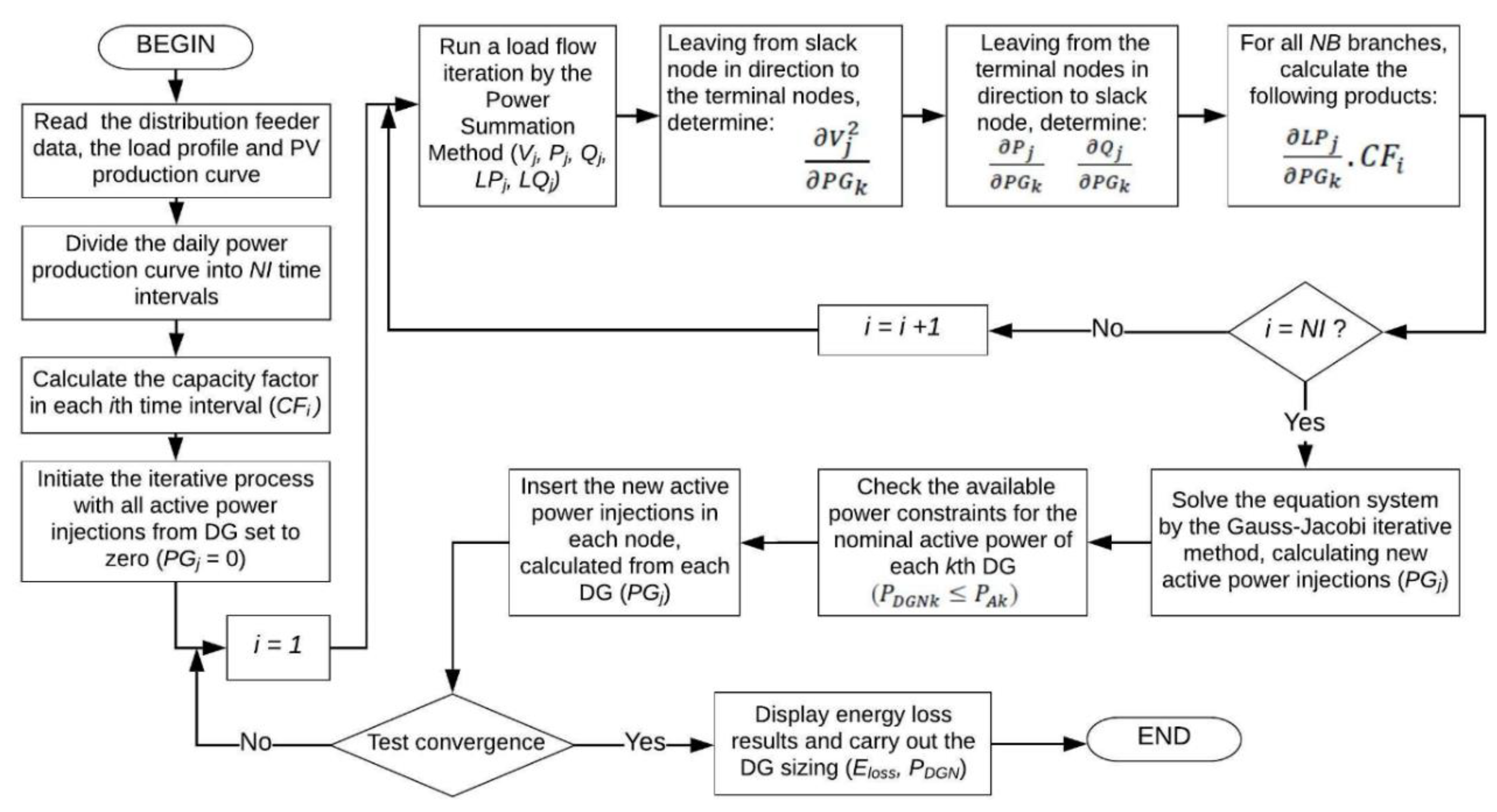
3.3. Solution Procedure

The method adopted for solving the distribution system power flow problem was suggested in [27,28], using the power summation algorithm, which consists in reducing the modelled systems to only two nodes, starting from the substation (slack bus), where the voltage magnitude is known and from the power on the second node, represented by the summation of all powers from the nodes downstream of slack bus. For this purpose, (8) is used, relating the node voltage at the side of the load, V_j, with the known voltage in the node at the side of the source, V_S.

To calculate the feeder’s energy losses gradient in relation to the generator nominal power, $\frac{\partial E_{loss}}{\partial P_{DGNk}}$, it is necessary to obtain $\frac{\partial V_j^2}{\partial P{G}_k}$, in (16), from the knowledge of the partial derivatives $\frac{\partial V_s^2}{\partial P{G}_k}$, $\frac{\partial P_j}{\partial P{G}_k}$ and $\frac{\partial Q_j}{\partial P{G}_k}$. The partial derivatives for the active power summation, $\frac{\partial P_j}{\partial P{G}_k}={{\displaystyle \sum }}_{m=1}^{NBd}\frac{\partial P{G}_m}{\partial P{G}_k}+{{\displaystyle \sum }}_{m=1}^{NBd}\frac{\partial L{P}_m}{\partial P{G}_k}$, and reactive power summation, $\frac{\partial Q_j}{\partial P{G}_k}={{\displaystyle \sum }}_{m=1}^{NBd}\frac{\partial L{Q}_m}{\partial P{G}_k}$, are then calculated. The solutions process must consider that the terms ${{\displaystyle \sum }}_{m=1}^{NBd}\frac{\partial P{G}_m}{\partial P{G}_k}$ are calculated according to the following situations: $\frac{\partial P{G}_m}{\partial P{G}_k}=1$, if the k node is downstream to the j node; $\frac{\partial P{G}_m}{\partial P{G}_k} = 0$, if the k node is upstream to the j node.

The terms ${{\displaystyle \sum }}_{m=1}^{NBd}\frac{\partial L{P}_m}{\partial P{G}_k}$ and ${{\displaystyle \sum }}_{m=1}^{NBd}\frac{\partial L{Q}_m}{\partial P{G}_k}$ are obtained from the previous iteration of solution algorithm. Therefore, the calculation begins by obtaining their values, from the end to the start of the feeder (backward process), where the partial derivatives of the losses with relation to the injected power by the generators are null, since there are no lines after the last node. The $\frac{\partial V_s^2}{\partial P{G}_k}$ values are obtained starting at the opposite direction (forward process), i.e., from the slack bus, where the voltage will not be influenced by the injected DG power.

To solve the energy losses minimization problem, the Gauss-Jacobi iterative method is adopted, starting with the application of initial conditions to the control variable vector, x. For this, according to the solution procedures, demonstrated in the Appendix B, the general matrix form is obtained from expressions (32) and (33), as follows:

$$\left[\begin{array}{cccc}{\beta }_{11}& \dots & {\beta }_{1n}& -\left[C{F}_i+dL{P}_i\right]\\ ⋮& \ddots & ⋮& ⋮\\ {\beta }_{n1}& \dots & {\beta }_{nn}& -\left[C{F}_i+dL{P}_i\right]\\ 1& \dots & 1& 0\end{array}\right]·\left[\begin{array}{c}\begin{array}{c}P{G}_1\\ ⋮\\ P{G}_n\end{array}\\ \lambda \end{array}\right]=\left[\begin{array}{c}{\sigma }_1\\ ⋮\\ {\sigma }_n\\ P_{con}\end{array}\right],$$

(34)

where $dL{P}_i=C{F}_i{{\displaystyle \sum }}_{j=1}^{NB}\left(\frac{\partial L{P}_j}{\partial P{G}_k}\right)$ and the coefficients ${\beta }_{11},\dots ,{\beta }_{nn}$, to n = NB branches are written as: ${\beta }_{kj}=\left({\phi }_{1k}\frac{2R_1\left(f_{1k}+dLP{1}_i\right)}{V_1^2}+{\phi }_{2k}\frac{2R_2\left(f_{2k}+dLP{2}_i\right)}{V_2^2}+\dots +{\phi }_{jk}\frac{2R_j\left(f_{jk}+dLP{j}_i\right)}{V_j^2}\right)$, with $dLP{j}_i={{\displaystyle \sum }}_{m=1}^{NBd}\left(\frac{\partial L{P}_m}{\partial P{G}_k}C{F}_i\right)$. The ${\sigma }_1,\dots ,{\sigma }_n$ values are calculated as in (31) and $P_{con}={{\displaystyle \sum }}_{j=1}^{NB}P{L}_j+{{\displaystyle \sum }}_{j=1}^{NB}L{P}_j$ is defined as the active power consumed by the loads and in the form of line losses.

For the entire insolation period, with i = 1, 2, …, NI intervals, (34) is rewritten in its general matrix form as:

$$\left\{{{\displaystyle \sum }}_{i=1}^{NI}\left[\begin{array}{cccc}{\beta }_{{\left(11\right)}_i}& \dots & {\beta }_{{\left(1n\right)}_i}& -\left[C{F}_i+dL{P}_i\right]\\ ⋮& \ddots & ⋮& ⋮\\ {\beta }_{{\left(n1\right)}_i}& \dots & {\beta }_{{\left(nn\right)}_i}& -\left[C{F}_i+dL{P}_i\right]\\ 1& \dots & 1& 0\end{array}\right]\right\}·\left[\begin{array}{c}\begin{array}{c}P{G}_1\\ ⋮\\ P{G}_n\end{array}\\ \lambda \end{array}\right]={{\displaystyle \sum }}_{i=1}^{NI}\left[\begin{array}{c}{\sigma }_{\left(1\right)}{}_i\\ ⋮\\ {\sigma }_{\left(n\right)}{}_i\\ P_{con}{}_i\end{array}\right].$$

(35)

The matrix Equation (35) composes the system of resolution of the minimization problem, where ${\sigma }_{\left(1\right)}{}_i , \dots , {\sigma }_{\left(n\right)}{}_i$ values, as well as the term $P_{con}{}_i$, in its terms ${{\displaystyle \sum }}_{j=1}^{NB}L{P}_j$, are dependent on the injected power values, PG_j, which can be solved by the Gauss-Jacobi iterative method. Thus, from the initial conditions for the distribution feeder, the values for the terms ${\sigma }_{\left(1\right)}{}_i , \dots , {\sigma }_{\left(n\right)}{}_i$, $P_{con}{}_i$, are calculated and then added up, for i = 1, 2, …, NI intervals. The variables $P{G}_1, \dots , P{G}_n, \lambda$ are then calculated by the inversion of their coefficient matrixes, updating the terms ${\sigma }_{\left(1\right)}{}_i , \dots , {\sigma }_{\left(n\right)}{}_i$, $P_{con}{}_i$ for each iteration, until the convergence of the algorithm is reached. Each active power inputted by the k-th generator, PG_k, found by the iterative method and calculated at the end of the NI intervals, is converted to match the nominal power of a corresponding k-th PV generator P_DGNk from the CF_i. factor. The solution method for the optimization problem is presented in the flowchart displayed in Figure 3.

4. Discussion

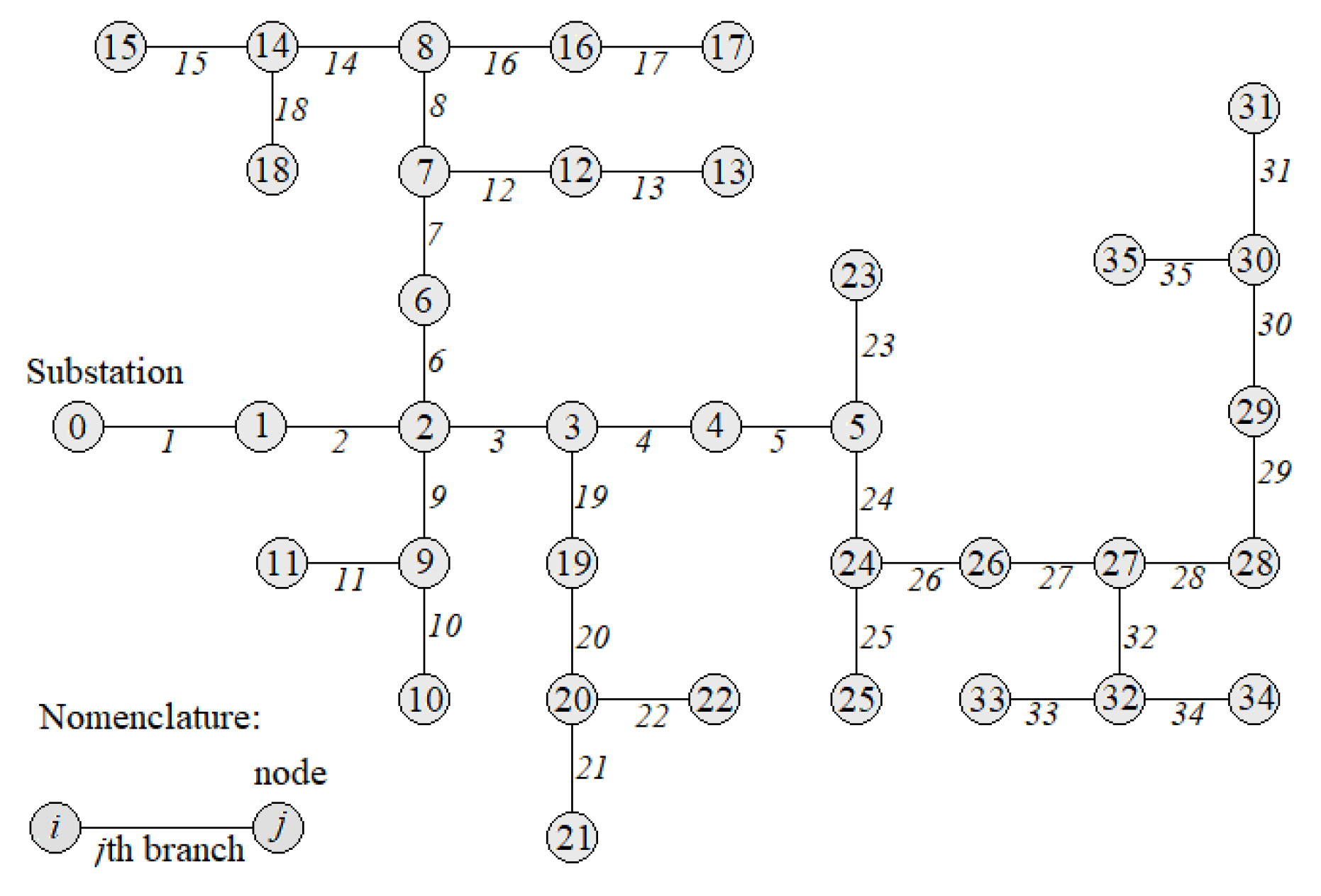
4.1. Case Study and Test System

The optimization method was evaluated for the IEEE 37-bus test system, whose characteristics are described in [30]. This system was adapted to the 36-bus system presented in Figure 4, from the grouping of two load buses and increased loading, by multiplying the load by a factor of 4. The name adopted for the branch and node follows the suggestion in [27], where the number of each load side node, or receiving node, j, is the same as the branch it is attached to, for j = 1, 2, …, NB, as displayed in Figure 4.

As a case study, the suggested methodology is evaluated by a radial distribution feeder, since this is the typical operation setting in the Brazilian system of medium voltage distribution. Moreover, the choice for a radial test system is related to the method adopted for load flow solution, which is the power summation method, and to the gradient calculations form, or tree gradient calculation, which uses the network’s radial typology features. It should be emphasized that, as for the Brazilian system, the meshed grids typically operate under a low voltage, and that the power summation method adaptation is not efficient. A triphasic radial distribution system was presumed, represented by single line diagram sections, in accordance to the electrical equivalent used in [27,28]. As the evaluated feeder’s distribution rated voltage is 13.8 kV, the line shunt capacitances were not taken in account.

According to [26], the Brazilian Normative Resolution from the Brazilian Electricity Regulatory Agency outlines the DG access conditions and implants the electrical power compensation system, whose decision to install the PV generation system is taken by the electrical power consumer. Thus, the power distributor company has no control over the DG’s optimal siting. Considering the stochastic nature of the PV generation connection problem, we presumed herein that all of the test system’s load buses can be PV generated, since the decision to install a PV system comes from the prosumers connected to the buses, i.e., due to the diffuse PV generation penetration, we considered the possibility of active power generation in each terminal node from each of the feeder’s branches. As defined in Section 2, the loads at the systems’ buses were presumed to have constant power and their loads were measured for each Δt_i interval in the insolation period, calculating the LF_i factors, in compliance with (3).

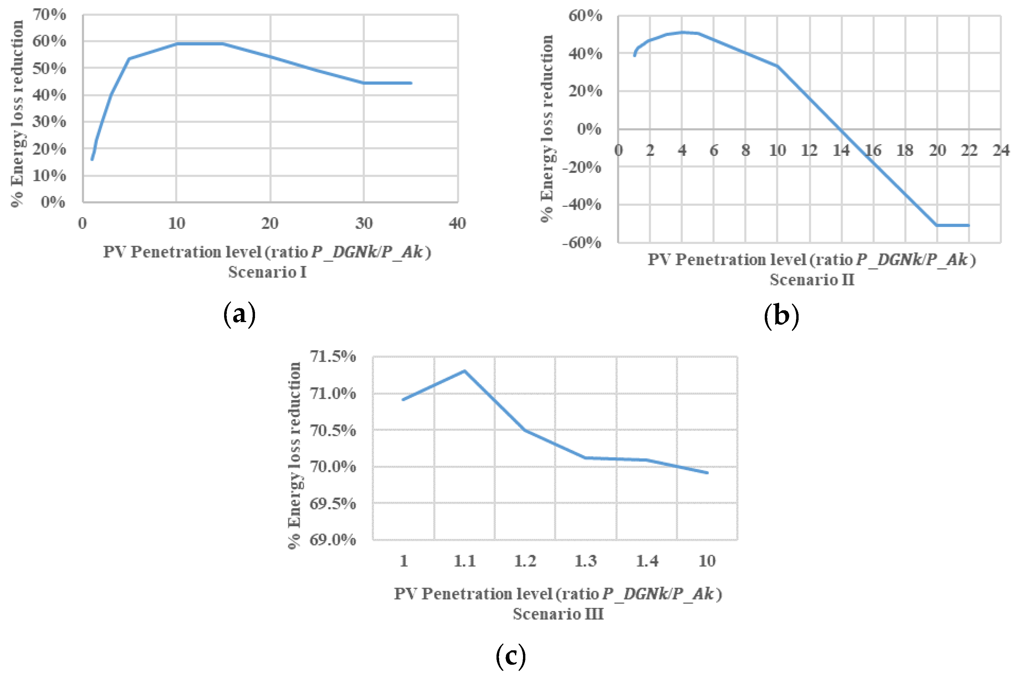
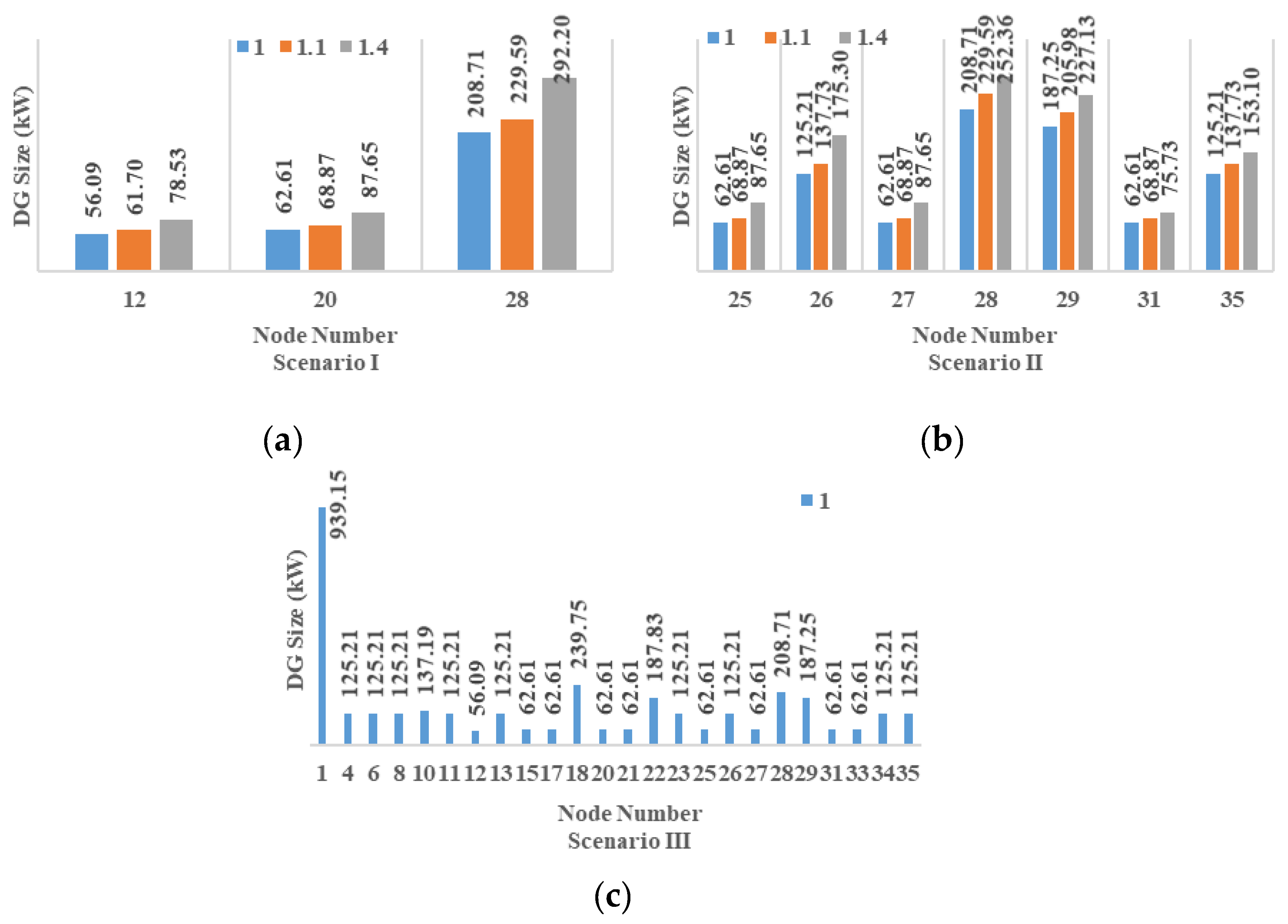
4.2. Numerical Results

In order to demonstrate the effectiveness of the proposed methodology, three location and PV generator integration scenarios were considered in the system presented in Figure 4, aside from the base scenario, in which there is no allocated DG in the system. Scenario I considers the existence of only three nodes with PV generation, diffusely distributed and with distinct feeder derivations. In Scenario II, PV generation is concentrated in a set of neighboring nodes in a single feeder derivation. Finally, the existence of uniform distributed PV generation is presumed for all of the feeder’s load nodes in Scenario III, in a context of wide DG integration. Different DG penetration levels were defined for each proposed scenario, from the limits for the relation between the generation installed power (P_DGNk) and the power provided for the consumer unity (P_Ak), as described in Section 2.

The algorithm proposed for this study was implemented using the free source software Scilab, in which the scenarios were simulated in order to obtain the energy losses and slack bus flow minimization, as presented in

Table 1. Summary of the IEEE 37-bus system results in different DG placement scenarios.

Topology	Ratio Limit PDGNk/PAk	Total System Energy Losses (kWh)	Energy through the Slack Bus (MWh)	Total DG Size (kW)
Base case		72.810	31.242	0.00
Scenario I (DG location in nodes 12, 20, 28)	1.0	61.137	28.928	327.42
	1.1	60.077	28.696	360.16
	1.2	59.037	28.465	392.90
	1.5	56.033	27.771	491.13
	2.0	51.418	26.615	654.84
	3.0	43.655	24.305	982.25
	5.0	33.973	19.690	1637.09
	10	29.917	13.080	2576.00
	15	29.879	8.906	3169.48
	20	33.207	4.735	3763.00
	25	37.135	1.857	4170.06
	30	40.495	0.000	4437.61
	35	40.495	0.000	4437.61
	without constraint	40.495	0.000	4437.61
Scenario II (DG location in nodes 25, 26, 27, 28, 29, 31, 35)	1	44.765	25.347	834.22
	1.1	43.101	24.759	917.64
	1.2	41.642	24.170	1001.06
	1.3	41.155	23.955	1033.88
	1.4	40.769	23.778	1058.92
	1.5	40.397	23.602	1083.97
	1.6	40.039	23.425	1109.02
	1.7	39.694	23.249	1134.06
	1.9	39.045	22.896	1184.16
	2.1	38.450	22.543	1234.25
	2.5	37.423	21.838	1334.44
	3.0	36.441	20.956	1459.67
	4.0	35.488	19.194	1710.13
	5.0	35.834	17.499	1952.17
	10	48.602	10.907	2891.44
	15	79.653	4.333	3830.70
	20	109.929	0.110	4446.09
	22	110.028	0.000	4447.50
	without constraint	110.028	0.000	4447.50
Scenario III (DG location in nodes 1, 4, 6, 8, 10, 11, 12, 13, 15, 17, 18, 20, 21, 22, 23, 25, 26, 27, 28, 29, 31, 33, 34, 35)	1	21.176	5.986	3583.76
	1.1	20.890	3.465	3942.14
	1.2	21.485	0.945	4300.51
	1.3	21.760	0.297	4391.12
	1.4	21.780	0.246	4397.96
	10	21.905	0.050	4439.80
	without constraint	21.905	0.050	4439.80

.

The combination of the DG integration scenarios and the power penetration levels, from the different limits for the relation $\frac{P_{DGNk}}{P_{Ak}}$, resulted in twenty-two scenarios, also considering the integration condition without the available power constraint in the simulation. Thus, the system’s total energy losses and slack bus energy flow calculated for the daily insolation period, as well as the PV active power generation sizing for each scenario, are presented in Table 1. For the base scenario, the feeder losses and slack bus energy flow are, respectively, 72.810 kWh and 31.242 MWh. For the $\frac{P_{DGNk}}{P_{Ak}}\le 1$ limit, these values were minimized: for Scenario I, at 61.137 kWh and 28.928 MWh; Scenario II, at 44.765 kWh and 25.347 MWh; and, for Scenario III, at 21.176 kWh and 5.986 MWh, respectively.

Also, as displayed in Table 1, with the increase of the relation $\frac{P_{DGNk}}{P_{Ak}}$ limits, the energy losses and the slack bus energy flow continue to decrease, up to a certain amount, in all three scenarios. Since the Lagrange augmented objective function in (23) incorporates the concurrent functions of minimizing system energy losses and the slack bus energy flow, we can state that the problem therefore has multiple objectives. Thus, Table 1 displays the increase in feeder energy losses, with a high rate of slack bus energy flow decrease: in Scenario I, at 33.207 kWh and 4.735 MWh; in Scenario II, at 48.602 kWh and 10.907 MWh; and in Scenario III, at 21.485 kWh and 0.945 MWh, respectively. By removing the available power constraint, the energy in the slack bus is minimized to values approaching zero. However with an increase in feeder energy losses to 40.495 kWh in Scenario I, 110.028 kWh in Scenario II and 21.905 kWh in Scenario III.

The decreases in feeder energy losses in the daily PV generation during the insolation period were evaluated for a condition of increasing DG power penetration, starting from higher increase rates for the $\frac{P_{DGNk}}{P_{Ak}}$ limits. The reduction in energy losses in Scenario I, where the percentage reduction begins at roughly 16% and rises to nearly 60%, is displayed in Figure 5a. By releasing the problem from the available power constraint and higher PV penetration, the reduction stabilizes at $\frac{P_{DGNk}}{P_{Ak}}=10$ (Figure 5a), followed by a slow increase in feeder losses. Thus, Scenario I, with only three DG allocation nodes, displays a drop in the percentage reduction, which then stabilizes at higher PV penetration levels.

Figure 5b presents the reduction curve for Scenario II, where the initial reduction is close to 40%, even though higher PV penetration levels induce the return of loss rates to those in the base scenario and, thereafter, an increase in the distribution feeder’s energy losses (crossing point $\frac{P_{DGNk}}{P_{Ak}}=14$). In Scenario III, Figure 5c, the initial energy losses reduction is significantly higher than those from the previous scenarios, close to 71%, with reduction stabilization of around 70%, reaching the optimal energy losses minimization for this scenario.

The optimal PV generation sizing for Scenarios I and II are displayed in Figure 6a,b, respectively. They indicate the increase in nominal power generation allocated to each node, in line with the increase of the available power relations (1, 1.1 and 1.4). Figure 6c presents the DG sizing of the PV type for Scenario II, but only for the relation $\frac{P_{DGNk}}{P_{Ak}}\le 1$. The optimal sizing for the nodes shared by all scenarios is obtained using the same nominal allocated PV generation power, thus being restricted to available power. In addition, the nodes displaying higher installed loads in the 36-bus test system present higher nominal PV generation power, as in the case of node 1 in Scenario III, Figure 6c, with PV generation sized as 939.15 kW.

The daily PV energy production curve and the distribution feeder’s load curve were divided into ten intervals for the entire insolation period.

Table 2. Capacity factors and load factors.

Time Intervals (i)	1	2	3	4	5	6	7	8	9	10
Capacity Factor (CFi)	0.200	0.660	0.836	0.940	0.986	0.965	0.887	0.757	0.538	0.264
Load Factor (LFi)	0.894	0.894	0.984	0.990	0.971	0.932	0.948	0.979	0.983	0.940

displays the PV generation capacity and distribution feeder load factor timetable calculated for each Δt_i = 1 h, used in the optimization algorithm.

Table 3. Voltage before and after DG placement in the IEEE 37-bus system.

Topology	Voltage before and after DG Location (pu)
	Min	Max
Base Case	0.9935	1.0000
Scenario I	0.9939	1.0000
Scenario II	0.9945	1.0000
Scenario III	0.9949	1.0000

highlights the minimum and maximum voltages for the 36-bus system before and after DG sizing and installation, for the base case and all assessed scenarios. The voltages are all within reasonable limits, with a maximum voltage of 1.00 pu, even after DG integration. The technical limits for the cables in each of the feeder lines were also assessed, and none exceeded current limits. The voltage dependence on the distribution network in relation to the power that is effectively generated by each PV generator was taken into account in the problem approach, according to the solution procedure presented. However, in the simulations and in the numerical results, we confirmed that the operational voltage limits in the nodes didn’t become active. Since the Lagrange’s augmented objective function suggested includes activities to minimize the energy losses in the feeder as well as the energy flow in the slack bus, we confirmed that the network currents were reduced, and the voltages always operated near their nominal value.

In order to assess the proposed methodology sensibility concerning the sizing of the PV generation nominal power, the scenarios were simulated to obtain the minimization of energy loss and flow in the slack bus under decrease and increase of the typical daily production curve. The simulation results are presented in

Table 4. Summary of the IEEE 37-bus system results considering three PV production levels.

Topology	PV Production Level	Total System Energy Losses (kWh)	Energy through the Slack Bus (MWh)	Total DG Size (kW)
Base Case		72.810	31.242	0.00
Scenario I Without constraint (ratio limit)	Typical	40.495	0.000	4437.61
	Minimum	40.495	0.000	5547.02
	Maximum	40.495	0.000	3698.01
Scenario II Without constraint (ratio limit)	Typical	110.028	0.000	4447.50
	Minimum	110.028	0.000	5559.38
	Maximum	110.028	0.000	3706.25
Scenario III Without constraint (ratio limit)	Typical	21.905	0.050	4439.80
	Minimum	21.882	0.024	5541.04
	Maximum	21.888	0.001	3692.93

, which considers three levels of PV generation daily production (typical, minimum and maximum). It is possible to see that the system’s total energy losses and energy flow in the slack bus are approximately the same for the three levels of PV production in the same scenario, since the system’s operating point is the same. However, the PV generation nominal power sized changes in comparison to the typical daily production curve and presents a relationship that is inversely proportional in relation to the PV production’s minimum and maximum levels.

5. Conclusions

Studies aiming at the analyses of possible impacts of a higher renewable distributed generation penetration in distribution systems have great relevance. To this end, both conventional techniques and metaheuristic algorithms for optimal renewable DG integration are currently being reviewed. The analytical method proposed herein makes the solution feasible for up to two iterations using the Gauss-Jacobi method and Lagrange multipliers. In addition, the proposed optimization method using gradients ensures better convergence, since it does not use the arbitrary step as in the pure gradient method, for situations where the search for an exact linear solution is computationally unfeasible. This method also ensures less computational effort, since it does not involve the Hessian matrix, as required by Newton’s method.

The determination of optimal PV generator nominal power, considering capacity and variable load factors during the insolation period, allows for a more thorough examination of the loss minimization problem, since it does not analyze only load peak conditions in a single demand and generation scenario.

The energy balance constraint limit, which aims for energetic feeder independence alongside the Lagrange augmented optimal function transformed the minimization problem into a multi-objective one, since it incorporates the concurrent functions of reducing both feeder energy losses and slack bus energy flow. Thus, feeder independence is achieved in some of the simulated scenarios, but with increased energy losses. This study demonstrates that available power constraint limits the installed nominal PV power, reducing the benefits of loss reduction in a system with few and disperse generation buses (Scenario I). The simulations also indicate that higher power limits for generation induce higher loss reduction rates up to the different limits observed in each scenario. A higher concentration of PV generators in a set of feeder-neighboring nodes (Scenario II) led to a reduction in the operational efficiency of the distribution network, with subsequent energy losses. Only the uniform PV units distribution (Scenario III) was able to maintain a stable energy loss reduction rate.

These differences between loss reduction curves reflect the effects of the DG location in the feeder. A higher concentration of PV generator in a set of feeder-neighboring nodes is less efficient for energy loss reduction. The analysis of these scenarios reflects the condition in which sets of consumer units presenting better socioeconomic background and are, therefore, potential PV generation consumers, have the potential to cause a decrease in the distribution network operation efficiency. Suggestion for improving these conditions include the implementation of smart grid controls, changing strategic company planning for renewable DG integration and implementing public policies to reduce asymmetries from regarding the benefits of access to PV generation.

References

1. Shaukat, N.; Ali, S.M.; Mehmood, C.A.; Khan, B.; Jawad, M.; Farid, U.; Ullah, Z.; Anwar, S.M.; Majid, M. A survey on consumers empowerment, communication technologies, and renewable generation penetration within Smart Grid. Renew. Sustain. Energy Rev. 2018, 81, 1453–1475. [Google Scholar] [CrossRef]
2. Kakran, S.; Chanana, S. Smart operations of smart grids integrated with distributed generation: A review. Renew. Sustain. Energy Rev. 2018, 81, 524–535. [Google Scholar] [CrossRef]
3. Arvesen, A.; Hauan, I.B.; Bolsøy, B.M.; Hertwich, E.G. Life cycle assessment of transport of electricity via different voltage levels: A case study for Nord-Trøndelag county in Norway. Appl. Energy 2015, 157, 144–151. [Google Scholar] [CrossRef]
4. Squires, R.B. Economic Dispatch of Generation Directly from Power System. Trans. Am. Inst. Electr. Eng. Part III Power Appar. Syst. 1960, 79, 1235–1244. [Google Scholar]
5. Dopazo, J.F.; Klitin, O.A.; Stagg, G.W.; Watson, M. An optimization technique for real and reactive power allocation. Proc. IEEE 1967, 55, 1877–1885. [Google Scholar] [CrossRef]
6. Dommel, H.W.; Tinney, W.F. Optimal power Load Flow Solutions. IEEE Trans. Power Appar. Syst. 1968, PAS-87, 1866–1876. [Google Scholar] [CrossRef]
7. Rau, N.S.; Wan, Y.H. Optimum Location of Resources in Distributed Planning. IEEE Trans. Power Syst. 1994, 9, 2014–2020. [Google Scholar] [CrossRef]
8. Ehsan, A.; Yang, Q. Optimal integration and planning of renewable distributed generation in the power distribution networks: A review of analytical techniques. Appl. Energy 2018, 210, 44–59. [Google Scholar] [CrossRef]
9. Abdmouleh, Z.; Gastli, A.; Ben-Brahim, L.; Haouari, M.; Al-Emadi, N.A. Review of optimization techniques applied for the integration of distributed generation from renewable energy sources. Renew. Energy 2017, 113, 266–280. [Google Scholar] [CrossRef]
10. Singh, B.; Sharma, J. A review on distributed generation planning. Renew. Sustain. Energy Rev. 2017, 76, 529–544. [Google Scholar] [CrossRef]
11. Mahmoud Pesaran, H.A.; Huy, P.D.; Ramachandaramurthy, V.K. A review of the optimal allocation of distributed generation: Objectives, constraints, methods, and algorithms. Renew. Sustain. Energy Rev. 2017, 75, 293–312. [Google Scholar] [CrossRef]
12. Sheng, W.; Liu, K.Y.; Liu, Y.; Meng, X.; Li, Y. Optimal Placement and Sizing of Distributed Generation via an Improved Nondominated Sorting Genetic Algorithm II. IEEE Trans. Power Deliv. 2015, 30, 569–578. [Google Scholar] [CrossRef]
13. Nor, N.M.; Ali, A.; Ibrahim, T.; Romlie, M.F. Battery Storage for the Utility-Scale Distributed Photovoltaic Generations. IEEE Access 2017, 6, 1137–1154. [Google Scholar] [CrossRef]
14. Ganguly, S.; Samajpati, D. Distributed generation allocation on radial distribution networks under uncertainties of load and generation using genetic algorithm. IEEE Trans. Sustain. Energy 2015, 6, 688–697. [Google Scholar] [CrossRef]
15. Marinopoulos, A.G.; Alexiadis, M.C.; Dokopoulos, P.S. Energy losses in a distribution line with distributed generation based on stochastic power flow. Electr. Power Syst. Res. 2011, 81, 1986–1994. [Google Scholar] [CrossRef]
16. Abu-Mouti, F.S.; El-Hawary, M.E. Optimal Distributed Generation Allocation and Sizing in Distribution Systems via Artificial Bee Colony Algorithm. IEEE Trans. Power Deliv. 2011, 26, 2090–2101. [Google Scholar] [CrossRef]
17. Bhullar, S.; Ghosh, S. Optimal integration of multi distributed generation sources in radial distribution networks using a hybrid algorithm. Energies 2018, 11, 628. [Google Scholar] [CrossRef]
18. Dahal, S.; Salehfar, H. Impact of distributed generators in the power loss and voltage profile of three phase unbalanced distribution network. Int. J. Electr. Power Energy Syst. 2016, 77, 256–262. [Google Scholar] [CrossRef]
19. Khaled, U.; Eltamaly, A.M.; Beroual, A. Optimal power flow using particle swarm optimization of renewable hybrid distributed generation. Energies 2017, 10, 1013. [Google Scholar] [CrossRef]
20. Sanjay, R.; Jayabarathi, T.; Raghunathan, T.; Ramesh, V.; Mithulananthan, N. Optimal allocation of distributed generation using hybrid Grey Wolf Optimizer. IEEE Access 2017, 5, 14807–14818. [Google Scholar] [CrossRef]
21. Li, Y.; Feng, B.; Li, G.; Qi, J.; Zhao, D.; Mu, Y. Optimal distributed generation planning in active distribution networks considering integration of energy storage. Appl. Energy 2018, 210, 1073–1081. [Google Scholar] [CrossRef]
22. Mena, A.J.G.; Martín García, J.A. An efficient approach for the siting and sizing problem of distributed generation. Int. J. Electr. Power Energy Syst. 2015, 69, 167–172. [Google Scholar] [CrossRef]
23. Mahmoud, K.; Yorino, N.; Ahmed, A. Optimal Distributed Generation Allocation in Distribution Systems for Loss Minimization. IEEE Trans. Power Syst. 2016, 31, 960–969. [Google Scholar] [CrossRef]
24. Viral, R.; Khatod, D.K. An analytical approach for sizing and siting of DGs in balanced radial distribution networks for loss minimization. Int. J. Electr. Power Energy Syst. 2015, 67, 191–201. [Google Scholar] [CrossRef]
25. de Medeiros Júnior, M.F.; Pimentel Filho, M.C. Optimal power flow in distribution networks by Newton’s optimization methods. In Proceedings of the IEEE International Symposium on Circuits and Systems, ISCAS ’98, Monterey, CA, USA, 31 May–3 June 1998; Volume 3, pp. 505–509. [Google Scholar]
26. ANEEL. Resolução n° 482, de 17 de abril de 2012, da ANEEL. Available online: http://www.aneel.gov.br/cedoc/ren2012482.pdf (accessed on 19 June 2017).
27. Cespedes, R.G. New method for the analysis of distribution networks. IEEE Trans. Power Deliv. 1990, 5, 391–396. [Google Scholar] [CrossRef]
28. Das, D.; Nagi, H.S.; Kothari, D.P. Novel method for solving radial distribution networks. IEE Proc. Gener. Transm. Distrib. 1994, 141, 291–298. [Google Scholar] [CrossRef]
29. Boyd, S.; Vandenberghe, L. Convex Optimization, 7th ed.; Cambridge University Press: New York, NY, USA, 2004; ISBN 9780521833783. [Google Scholar]
30. Kersting, W.H. Radial distribution test feeders. IEEE Trans. Power Syst. 1991, 6, 975–985. [Google Scholar] [CrossRef]
Figure 1. Daily power production curve for a real 84.2 kWp PV unit connected to a local distribution feeder.
Energies 12 01728 g001
Figure 2. System reduced to the s and j nodes.
Energies 12 01728 g002
Figure 3. Flowchart of the proposed energy losses minimization method using Lagrange multipliers.
Energies 12 01728 g003
Figure 4. Diagram of the 36-bus radial distribution feeder adapted from the IEEE 37-bus test system.
Energies 12 01728 g004
Figure 5. Energy losses reduction under a condition of increasing PV generation: (a) Scenario I; (b) Scenario II; (c) Scenario III.
Energies 12 01728 g005
Figure 6. Optimal PV generation sizing: (a) in Scenario I for ratios of 1, 1.1 and 1.4; (b) in Scenario II for ratios of 1, 1.1 and 1.4; (c) in Scenario III for a ratio of 1.
Energies 12 01728 g006