A New Hybrid Approach for Short-Term Electric Load Forecasting Applying Support Vector Machine with Ensemble Empirical Mode Decomposition and Whale Optimization

Abstract

Electrical power system forecasting has been a main focus for researchers who want to improve the effectiveness of a power station. Although some traditional models have been proved suitable for short-term electric load forecasting, its nature of ignoring the significance of parameter optimization and data preprocessing usually results in low forecasting accuracy. This paper proposes a short-term hybrid forecasting approach which consists of the three following modules: Data preprocessing, parameter optimization algorithm, and forecasting. This hybrid model overcomes the disadvantages of the conventional model and achieves high forecasting performance. To verify the forecasting effectiveness of the hybrid method, 30-minutes of electric load data from power stations in New South Wales and Queensland are used for conducting experiments. A comprehensive evaluation, including a Diebold-Mariano (DM) test and forecasting effectiveness, is applied to verify the ability of the hybrid approach. Experimental results indicated that the new hybrid method can perform accurate electric load forecasting, which can be regarded as a powerful assist in managing smart grids.

1. Introduction

Electric load forecasting acts an important part in power station operations, such as the expansion of power generation, dispatch scheduling of generation production, maintenance, and the insurance of continuously supplied electric power [1]. An accurate electric load forecasting model can not only assist the power station in the management of electricity and the arrangement of operations, but is also able to reduce the loss of auxiliary power, which enhances the stability and the economic benefits of the station. Inaccurate forecasting results, on the other side, can result in abundant electricity waste. For example, underestimated forecasting will raise the difficulty in supplying adequate electric resources, which raises the cost of the power station [2]. Therefore, to obtain a satisfying prediction result, the need to develop an accurate and effective electric load forecasting system is intensely high.

To obtain an accurate forecasting result for electric power stations, many short-term predicting methods were introduced, and those can mainly be classified into three categories: conventional methods, modern methods, and hybrid methods. Firstly, conventional methods include multi-linear regression analysis, time series, state space models, general exponential smoothing, and knowledge-based methods [3,4,5,6,7,8]. However, these methods cannot provide appropriate nonlinear exiting mathematical relationships to express actual electric loads. Secondly, modern methods are intelligent evolutionary algorithms, expert systems, neural networks, and fuzzy inference [9,10,11,12,13,14,15,16,17]. Intelligent algorithms and neural networks can obtain good performance because of their clear patterns, easy implementation, and strong ability to address the problem. Thirdly, hybrid forecasting methods, which are proposed to avoid the shortcomings in individual methods, have become more and more popular [18,19].

The procedure of traditional forecasting methods is precise, which are based on traditional mathematic ideas and theories, such as statistics, calculus, and modeling [20]. The main theory of trend extrapolation technology is to find the patterns in the given data to forecast future data based on the trend equation. Though the method is simple, it can obtain an accurate forecasting result for continuous electric load data. However, its accuracy can be greatly impacted by random load components, which is an inadequacy of the method [21]. Regression analysis is usually used in short-term electric data prediction [22]. This method has many advantages, such as a simple principle and a better quality of data, which leads to better precision. However, the selection of the main factors affecting power load in the model is difficult as many factors that affect the forecasting accuracy are hard to quantify. This model is lacking any self-study capability and the input variable and output variable cannot be revised automatically [23]. With years of development, the time series forecasting method has become a mature theory method and has been applied to power load forecasting [24]. The basic time series prediction models mainly include AR (auto regressive), MA (moving average), and ARMA (auto regressive moving average) [25]. Although the time series forecasting method has advantages, such as only requiring a small volume of historical data and small amounts and fasts speed of calculation, this method has certain limitations, such as its inability to reflect the influence of meteorological factors and how its forecasting accuracy will decrease with the increase of the prediction step [26]. An ANN (Artificial Neural Network) is a type of nonlinear simulation of the human brain information processing system with an intelligent processing process for an inaccurate variation trend, this method also has a good ability to adapt, is able to grasp information and keep on learning, and has good knowledge reasoning and self-optimization [27]. An expert system is a computer system based on the knowledge of the programming approach, mainly a software system, and the main components of an expert system include the inference engine of the system, the expert knowledge base, the explain interface, and the knowledge acquisition module. It is a program that has decision making capabilities based on reasoned knowledge, however, this method is limited by whether the expert knowledge is complete [28]. The grey forecasting method is an important technique in grey theory, which uses approximate differential equations to describe future tendencies for a time series [29]. Limitation of this method is that the greater the dispersion degree of data, the worse the forecasting accuracy. Although traditional forecasting methods and forecasting methods based on intelligent computing have their respective applications, it is difficult to obtain high accuracy prediction when utilizing one of them by itself [30]. In the literature related to forecasting [31,32,33], the forecasting results are not quite as good with any single forecasting model. The primary reason is that single forecasting models cannot extract the complicated factors in reality.

Recently, to overcome drawbacks of conventional methods, researchers focused more on hybrid or combined approaches. These approaches are usually made up of data pre-processing techniques, parameter optimization algorithms, and weighting-combined methods [34,35,36,37,38,39,40,41], which can enhance the accuracy of short-term electric load forecasting. For example, Wang et al introduced a combined approach using GPR (Gaussian process regression) and WT (wavelet transform) to combine individual models and identify noise in the original time series, the results of which indicated that the forecasting accuracy is improved with the combined model applied [34]. Liu et al utilized EMD (empirical mode decomposition) to decompose original data into IMFs (intrinsic mode function) for reconstructing a more stationary time series [40]. The performance of the model was verified by four case studies. A combined approach which applies BPNN (back propagation neural network), ARIMA (autoregressive integrated moving average model), and ANFIS (adaptive network-based fuzzy inference system) with optimized weights is proposed by Yang et al, which was also proved for higher accuracy by case studies [41]. Those discussed methods illustrated that hybrid and combined models can improve the effectiveness of forecasting, compared with conventional models [42,43,44].

Through the review of previous articles, the forecasting methods mentioned earlier all have several shortcomings. The drawbacks of those approaches are summed up as the following: (1) Traditional statistical methods cannot perform forecasting using data with high noise and fluctuation features, which electric load data usually have. This method is limited by the assumption of a smooth linear form time series. Furthermore, these traditional methods require great amounts of historical data to train for predicting, which shows the fact that these methods depend highly on a raw time series. When a raw time series changes unexpectedly, because of certain factors in the power stations, the accuracy of the forecasting will be relatively low [45]. (2) Artificial intelligence methods, which can be successfully utilized in forecasting, can capture non-linear features in raw data [46]. However, this method still has many drawbacks, such as a local optimum, over-fitting, and low convergence rate [47]. (3) Individual methods rarely focus on the data preprocessing technique, so they usually obtain a relatively low forecasting accuracy. Therefore, due to these disadvantages of conventional methods mentioned above, a hybrid approach, which can capture the hidden features in the electric load data and can be widely applied, needs extreme consideration in order to achieve accurate forecasting results. 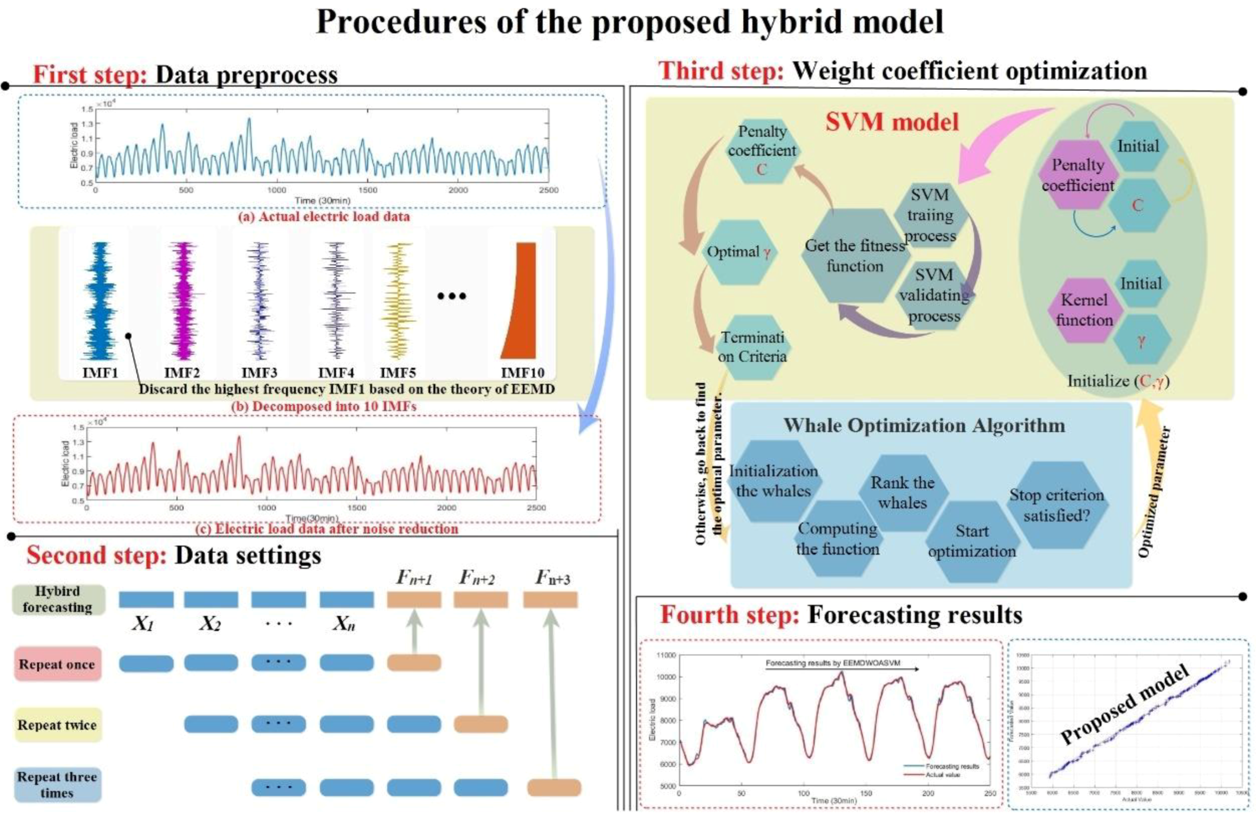[48]. This paper proposes a new hybrid approach combining ensemble empirical mode decomposition (EEMD), a Whale Optimization Algorithm (WOA), and a support vector machine (SVM).

The leading progress of this paper, in comparison with other works in the field of electric load prediction, is summarized as follows:

• The method introduced in this paper utilized a data preprocessing technique to improve the accuracy of the proposed approach. Raw electric load data is first broken down into sub-signals. Signals with high noise are taken away and the rest are reorganized into a more stationary series. In this way, the uncertainty and irregularity in the electric load data can be decreased and features in the electric load data can be better analyzed. Eventually, the performance of the proposed method is enhanced.
• The new model utilizes Whale Optimization to optimize key parameters in SVM before forecasting. Whale Optimization has the advantage of requiring few parameters and a strong problem-solving ability, which is an effective tool in global optimization. By using it, a support vector machine can greatly improve its predicting accuracy and avoid shortcomings in traditional approaches, such as dimensionality, local optima, and over-learning.
• To further test the performance of the hybrid model, traditional and hybrid models are used for comparison in the experiment. Comprehensive evaluations are applied, which include multi-step ahead forecasting performance evaluation metrics, such as error indexes, DM tests, and forecasting effectiveness, verifying the ability of the proposed model.
• The proposed approach can be an effective tool for an electric station. Experiments concluded in this paper are based on electric load data from two different power stations with two different time horizons. The results showed that the hybrid approach can enhance the accuracy of forecasting and is easily applied in different stations.

This paper is organized as follows. Section 2 introduces the required techniques and the proposed approach. Section 3 and Section 4 introduces the evaluation criterion and description of the experiment data sets. For Section 5, Section 6, and Section 7, experiments were conducted and the results and the significance of the hybrid model are analyzed in detail. Finally, Section 8 concludes the paper and gives a possible direction for future work.

2. Materials and Methods

In this section, the required tools in the proposed method and the testing techniques, including a DM test and forecasting effectiveness, are introduced. Then, the hybrid approach is presented.

2.1. Ensemble Empirical Mode Decomposition (EEMD)

EEMD, which is based on empirical mode decomposition (EMD) was originally presented by Wu and Huang [49]. The main idea of ensemble empirical mode decomposition is to solve issues of mode mixing with the application of noise feature in the raw data. The raw data are made up with true signals and noise. Using EEMD, a white noise is added in raw time series to assist in extracting the true features in the data. The process of EEMD is described as the following:

(1)

Adding a white noise in the raw electric load data;

(2)

According to procedures of EMD, break down the data with the white noise included into n oscillatory modes (IMFs);

(3)

Repeating the above-mentioned two steps by adding white noise to the data at various scales each time;

(4)

Calculating the average values of each IMF from the decomposition process to the establish final IMFs.

White noise, which is put into the original time series can give a reference range to help with reducing the noise. In this way, true IMFs is obtained from a raw time series.

Definition 1.

According to works of Wu and Huang, the ensemble number, the error tolerance, and the level of added noise is defined as follows:

$$N_{\epsilon }=\frac{{\epsilon }^2}{{\epsilon }_n^2}$$

(1)

where ε is the amplitude of added noise, ε_n represents standard deviation of error, and $N_{\epsilon }$ stands for the ensemble members’ value. In this paper, the value of ensemble members is 100. The standard deviation of white noise series is chosen to be between 0.1 and 0.2. The amplitude is fixed at 0.2.

2.2. Whale Optimization Algorithm

Whale optimization algorithm (WOA), first introduced by Mirjalili and Lewis [50], is inspired by wildlife activities and has been widely applied in engineering areas. To test its abilities of exploitation, analysis, avoiding local optima, and convergence, 29 test functions, along with 6 structural engineering questions, are applied in an experiment, the results of which showed that Whale Optimization Algorithm (WOA) is superior to many other optimization algorithms, such as Particle Swarm Optimization (PSO), Gravitational Search Algorithm (GSA), and so on [51,52,53]. The main theory of WOA is presented as the following:

2.2.1. Encircle the Prey

Definition 2.

Humpback whales can find locations of the prey and circle around it. As soon as the best search agent is located, the others will move to this best location. This encircling activity can be expressed as the following:

$$\overrightarrow{D}=|\overrightarrow{C}·{\overrightarrow{X}}^{\ast }\left(t\right)-\overrightarrow{X}\left(t\right)|,$$

(2)

$$\overrightarrow{X}\left(t+1\right)={\overrightarrow{X}}^{\ast }\left(t\right)-\overrightarrow{A}·\overrightarrow{D},$$

(3)

where t represents current iteration, $\overrightarrow{X}$ stands for whales’ location, and ${\overrightarrow{X}}^{\ast }$ is the prey’s location, while $\overrightarrow{A}$ and $\overrightarrow{C}$ are coefficient vectors, which are defined as the following:

$$\overrightarrow{A}=2\overrightarrow{a}·\overrightarrow{r}-\overrightarrow{a},$$

(4)

$$\overrightarrow{C}=2·\overrightarrow{r},$$

(5)

where $\overrightarrow{r}$ stands for a random vector between 0 and 1, while $\overrightarrow{a}$ decreases from 2 to 0 over the iterations.

2.2.2. Bubble-Net Strategy

In this part, two approaches are introduced to describe the bubble-net strategy, which humpback whales use to catch their prey.

(1) Shrinking encircle mechanism

This approach is obtained through reducing value of $\overrightarrow{a}$. Between the original and current best spot, the new location can be obtained by placing random $\overrightarrow{A}$ between −1 and 1.

(2) Spiral updating position

The equation which describes helix-shaped shift of whales is obtained as follows:

$$\overrightarrow{X}\left(t+1\right)={\overrightarrow{D}}^{\prime }·e^{bl}·\cos \left(2\pi l\right)+{\overrightarrow{X}}^{\ast }\left(t\right)$$

(6)

where ${\overrightarrow{D}}^{\prime }$ represents distance between the i^th whale and the prey, b is a logarithmic spiral form, and l is a random value in (−1,1). The WOA is set at a 50% possibility to choose between the shrinking encircling mechanism and the spiral updating position.

Definition 3.

The process which updates solutions in iterations is defined as follows:

$$\mathrm{X}\left(t+1\right)=\{\begin{array}{c}{\overrightarrow{D}}^{\prime }·e^{bl}·\cos \left(2\pi l\right)+{\overrightarrow{X}}^{\ast }\left(t\right) if p\ge 0.5\\ {\overrightarrow{X}}^{\ast }\left(t\right)-\overrightarrow{A}·\overrightarrow{D} if p<0.5\end{array}.$$

(7)

2.2.3. Search for Prey

When searching, the location of an agent is updated by a value, which is selected to replace the best result at random. The process increases the ability of exploration, for which the WOA achieves better performance. This process can be described as follows:

$$\overrightarrow{D}=|\overrightarrow{C}·{\overrightarrow{X}}_{rand}-\overrightarrow{X}|,$$

(8)

$$\overrightarrow{X}\left(t+1\right)={\overrightarrow{X}}_{rand}-\overrightarrow{A}·\overrightarrow{D}.$$

(9)

When $|\overrightarrow{A}|$ < 1, the best solution is selected. If $|\overrightarrow{A}|$ > 1, an agent is chosen at random. The WOA is stopped when it reaches the criterion of termination.

2.3. Support Vector Machine (SVM)

A support vector machine, as a state-of-the-art forecasting model, was first proposed by Vapnik [54]. Its feature of following the theory of statistical machine learning and structural risk minimization makes it more powerful than other conventional models in the work of finding the minimal upper bound generalization error, for which it is widely applied in fields of pattern identification, categorization, regression analyzation, and forecasting [55,56].

Definition 4.

Set a group of data ${\left\{x_i{d}_i\right\}}_i^n$, in which the n-dimensional input vector is defined as $x_i$, while the output is $d_i$. The SVM function is described as follows:

$$f\left(x\right)=w·\varphi \left(x\right)+b,$$

(10)

where $\varphi \left(x\right)$ stands for nonlinear mapping. The values w and b represent the weight and scalar of the vector, which are calculated by the following:

$$R_{SVMs}\left(C\right)=\frac{1}{2}||w^2||+C\frac{1}{n}{{\displaystyle \sum }}_{i=1}^{n}L\left(x_i,d_i\right),$$

(11)

where C stands for error’s penalty factor, $L\left(x_i,d_i\right)$ is loss function, and $C\frac{n}{2}{\displaystyle \sum }_{i=1}^{n}L\left(x_i,d_i\right)$ is the empirical error. The upper and lower excess deviations, ${\xi }_i$, ${\xi }_i^{\ast }$, are set as positive slack variables and optimization is calculated through following equations:

$$Minimize{R}_{SVMs}\left(w,{\xi }^{(\ast )}\right)=\frac{1}{2}||w^2||+C\frac{1}{n}{{\displaystyle \sum }}_{i=1}^n\left({\xi }_i+{\xi }_i^{\ast }\right),$$

(12)

$$Subject to\{\begin{array}{c}{d}_i-w\varphi \left(x_i\right)-b_i\le \epsilon +{\xi }_i\\ w\varphi \left(x_i\right)+b_i-d_i\le \epsilon +{\xi }_i^{\ast }\\ {\xi }_i,{\xi }_i^{\ast }\ge 0,i=1,\dots ,l\end{array}$$

(13)

where $w^2/2$ stands for term of regularization, $\epsilon$ is loss factor whose value is based on the input data’s rough precision, and l is number of elements in the input sample groups.

A Gaussian function is one of most effective core functions in terms of simplicity, efficiency, and reliable computing ability. Applying a Gaussian function as its core function, an SVM can capture complex features in the original sample.

Definition 5.

As a core function of an SVM, a Gaussian function is described as the following:

$$K\left(x_i,x_j\right)=exp\left(-\gamma x_i-x_j{}^2\right),$$

(14)

where γ is parameter of the kernel function and $x_i$ and $x_j$ are quantities of vectors in the tr input sample.

This paper set (γ, C) as key parameters affecting the precision of electric load prediction. A WOA is applied to optimize these two key parameters.

2.4. Testing Method

To further certify the ability of the proposed approach, a Diebold-Mariano (DM) test and forecasting effectiveness are utilized to test the effectiveness of the hybrid approach.

2.4.1. DM Test

A Diebold-Mariano (DM) test is applied for testing the significance of outperformance, from which forecasting results of the proposed model have been compared with other traditional methods [57,58,59].

A hypothesis test is described as the following:

$$H_0:E\left(d_h\right)=0,\forall n,$$

(15)

$$H_1:E\left(d_h\right)\ne 0,\exists n.$$

(16)

The statistic values of the DM test are obtained by the following:

$$DM=\frac{{{\displaystyle \sum }}_{h=1}^k\left(L\left({\epsilon }_{t+h}^{\left(A\right)}\right)-L\left({\epsilon }_{t+h}^{\left(B\right)}\right)\right)/k}{\sqrt{S^2/k}}{s}^2,$$

(17)

where ${\epsilon }_{t+h}$ represents error, $S^2$ stands for estimation for variance of $d_h=L\left({\epsilon }_{t+h}^{\left(A\right)}\right)-L\left({\epsilon }_{t+h}^{\left(B\right)}\right)$, and L is a loss function, measuring the accuracy of different models.

The test statistic DM is convergent in the standard normal distribution. The null hypothesis will be rejected if

$$|DM|>z_{\alpha /2},$$

(18)

where $z_{\alpha /2}$ is critical z-value of standard normal distribution and α stands for the level of significance.

2.4.2. Forecasting Effectiveness

Forecasting effectiveness is calculated by the sum of squared errors and through the mean and mean square deviation of the forecasting accuracy [60]. The kth-order forecasting effectiveness unit can be calculated as the following:

$$m^k={{\displaystyle \sum }}_{n=1}^N{Q}_n{A}_n^k,$$

(19)

where $Q_n$ stands for discrete probability distribution, in which ${\displaystyle \sum }_{n=1}^N{Q}_n=1$. The value ${\mathrm{A}}_n$ represents accuracy.

The k-order forecasting effectiveness can be defined as

$$\mathrm{H}\left(m^1,m^2,\cdots ,m^k\right).$$

(20)

2.5. The Proposed EEMD-WOA-SVM Approach

Based on the techniques discussed above, this paper proposes a method that combines data preprocessing techniques with optimization algorithms to improve the forecasting ability of SVM for electric load prediction. Procedures of the hybrid approach are shown in Figure 1. Original electric load data is first processed by the EEMD, which reduces noise in the raw time series to obtain more stationary data. The data after the noise reduction process is utilized for three-steps ahead forecasting, testing the forecasting ability of the hybrid approach. Next, as mentioned before, the accuracy of SVM depends highly on two key parameters, the penalty factor and the kernel parameter (γ, C). Whale optimization is applied to search these two parameters. Finally, forecasting results of each step are recorded for analyzation and comparison.

3. Forecasting Evaluation Criterion

To verify the performance of the hybrid model, a variety of indexes containing the mean absolute error (MAE), the average of absolute percentage error (MAPE), the square root of average of error square (RMSE), Willmott’s Index (WI), the Nash–Sutcliffe coefficient (E_NS), and the Legates and McCabe Index (E_LM) are utilized for comparison. These evaluation indexes are defined in

Table 1. The definition of error evaluation indexes.

Metric	Definition	Equation
MAE	Mean absolute error	$MAE=\frac{1}{N}{\displaystyle \sum _{i=1}^N}|y{p}_i-y_i|$
MAPE	Average of absolute percentage error	$MAPE=\frac{1}{N}{\displaystyle \sum _{i=1}^N}|\frac{y{p}_i-y_i}{y_i}|\times 100\%$
RMSE	Square root of average of error square	$RMSE=\sqrt{\frac{1}{N}{\displaystyle \sum _{i=1}^N}{\left(y{p}_i-y_i\right)}^2}$
WI	Willmott’s Index	$WI=1-\left[\frac{{{\displaystyle \sum }}_{i=1}^N{(y{p}_i-y_i)}^2}{{{\displaystyle \sum }}_{i=1}^N{(|y{p}_i-\overline{y}|+|y_i-\overline{y}|)}^2}\right], 0\le WI\le 1$
ENS	Nash–Sutcliffe coefficient	$E_{NS}=1-\left[\frac{{{\displaystyle \sum }}_{i=1}^N{(y{p}_i-y_i)}^2}{{{\displaystyle \sum }}_{i=1}^N{(y_i-\overline{y})}^2}\right], \infty \le E_{NS}\le 1$
ELM	Legates and McCabe Index	$E_{LM}=1-\left[\frac{{{\displaystyle \sum }}_{i=1}^N|y_i-y{p}_i|}{{{\displaystyle \sum }}_{i=1}^N|y_i-\overline{y}|}\right],\infty \le E_{LM}\le 1$

where N represents output sample group; y_i is the original electric load data; and yp_i is the forecasting results of the used models.

.

This paper used Windows 10 Professional operating system, on which Matlab2018a was utilized for conducting experiments. Specific details of the hardware used in this paper are the following: Intel Core i5-8400 2.80 GHz CPU, with 8 GB RAM.

4. Data Settings

To test the forecasting ability of the EEMD-WOA-SVM method, the electric load data from New South Wales (NSW) and Queensland (QLD) were utilized to construct experiments in this paper. The data used in this paper is divided into training and testing groups. A total of 75% of the data were in the training group while the rest were in testing. Data in New South Wales were recorded every 30 min from 1 January 2013 to 22 February 2013. For the electric load data in Queensland, they were recorded every one hour from 1 January 2013 to 27 April 2013. In the experiment, the data collected from the two stations were used to perform electric load forecasting.

5. Experiments

The raw electric load data were first preprocessed by EEMD. Figure 2 shows the noise reduction process using the electric load data from New South Wales. The original electric load series are broken down into 10 IMFs. Basing on the theory of EEMD, the first IMF, which contains high noise, was eliminated from the raw time series for a more stationary data group. To verify the improvement the EEMD technique makes to the forecasting model, Support Vector Machine forecasting models using three different algorithms (Particle Swarm Optimization, Cuckoo Search Algorithm, Whale Optimization Algorithm) were used to conduct the experiment, with 30 min electric load data from New South Wales. First, these models performed forecasting without the preprocessing technique and the results are recorded in

Table 2. Forecasting results of different models without EEMD using 30 min electric load data from New South Wales.

Model	Step	MAE	MAPE	RMSE	WI	ENS	ELM
PSOSVM	1-step	44.1815	1.5896	185.3513	0.9441	0.7859	0.5790
	2-step	51.3622	2.7720	240.4546	0.8816	0.5245	0.3529
	3-step	79.5895	3.9541	331.7354	0.8013	0.4238	0.2723
CSOSVM	1-step	35.6786	1.2398	135.0801	0.9433	0.8174	0.5674
	2-step	41.0787	2.3624	193.7813	0.9183	0.6799	0.4140
	3-step	91.6241	4.2336	256.7493	0.8876	0.5048	0.2315
WOASVM	1-step	30.1841	1.0279	124.2342	0.9724	0.9103	0.7052
	2-step	38.3962	2.0719	169.5034	0.9466	0.7528	0.5215
	3-step	64.6579	3.4814	220.8291	0.9082	0.5816	0.3310

. Then, after the electric load data were processed by the EEMD, the obtained time series were used to perform the forecasting with these three models and the results were recorded, as shown in

Table 3. Forecasting results of different models with EEMD using 30 min electric load data from New South Wales.

Model	Step	MAE	MAPE	RMSE	WI	ENS	ELM
EEMDPSOSVM	1-step	41.2483	1.2536	162.3286	0.9695	0.8516	0.6324
	2-step	45.4937	2.0583	203.5379	0.9284	0.7042	0.4703
	3-step	64.7734	3.1172	283.8547	0.8805	0.5589	0.2277
EEMDCSOSVM	1-step	31.1964	1.0196	130.3385	0.9721	0.8937	0.6903
	2-step	37.4187	1.8234	174.5614	0.9215	0.7753	0.5146
	3-step	72.6024	3.1321	221.9207	0.8649	0.5849	0.3403
EEMDWOASVM	1-step	28.4251	0.8649	110.3028	0.9882	0.9421	0.7427
	2-step	35.3962	1.3482	154.4275	0.9672	0.8933	0.6891
	3-step	58.8694	2.1361	185.5310	0.9327	0.7458	0.4992

.

The ability of the WOA was also tested in the experiment. To verify the ability of WOA, particle swarm optimization (PSO) and a Cuckoo Search Algorithm (CSO) was applied in experiment. These three algorithms were all applied in the SVM model separately the conduct electric load prediction using the 30 min time series from New South Wales. Forecasting results are recorded in Table 2 and Table 3.

Multistep forecasting, which uses the method of removing old input data in each step is utilized in the experiment. Through using previous output instead of actual data, the multistep-ahead method predicts the next electric load value through this circulation [61]. Three-steps forecasting is applied in this paper. The hybrid method was tested and analyzed based on the results of three-steps ahead forecasting.

Table 4. Forecasting results of the proposed model and some traditional models using 30 min electric load data from New South Wales.

Model	Step	MAE	MAPE	RMSE	WI	ENS	ELM
BPNN	1-step	61.4766	2.4468	120.5819	0.9684	0.8907	0.6649
	2-step	102.6827	3.6791	233.8639	0.9511	0.8552	0.5734
	3-step	152.9354	4.9265	305.1517	0.8992	0.7148	0.4785
ARIMA	1-step	79.4672	3.3806	158.5784	0.9686	0.9047	0.7357
	2-step	142.7035	5.6058	278.7728	0.9119	0.6207	0.4864
	3-step	270.9721	6.9025	342.9586	0.8622	0.4879	0.2985
RBFNN	1-step	83.2925	2.5924	136.3627	0.9531	0.7917	0.6483
	2-step	106.4804	4.8720	208.5065	0.9042	0.5490	0.3210
	3-step	189.7480	5.2437	283.7569	0.8755	0.3816	0.2201
EEMDWOASVM	1-step	28.4251	0.8649	110.3028	0.9882	0.9421	0.7427
	2-step	35.3962	1.3482	154.4275	0.9672	0.8933	0.6891
	3-step	58.8694	2.1361	185.5310	0.9327	0.7458	0.4992

and

Table 5. Forecasting results of the proposed model and other traditional models using 60 min electric load data from Queensland.

Model	Step	MAE	MAPE	RMSE	WI	ENS	ELM
BPNN	1-step	119.8969	3.1382	149.6288	0.9483	0.8125	0.6235
	2-step	205.7309	4.4634	266.3948	0.9027	0.6316	0.4684
	3-step	272.5635	5.8783	331.0826	0.8573	0.4931	0.2977
ARIMA	1-step	132.6880	3.3396	183.2464	0.9486	0.8637	0.6881
	2-step	246.1020	4.0931	289.0470	0.9205	0.7122	0.4478
	3-step	310.1020	6.2143	385.6055	0.8833	0.5413	0.2581
RBFNN	1-step	135.9948	3.6645	173.1487	0.9408	0.8324	0.6489
	2-step	225.8553	5.2830	273.6628	0.9135	0.6720	0.4528
	3-step	301.5956	7.0080	353.4685	0.8949	0.5383	0.2758
EEMDWOASVM	1-step	115.5994	1.3249	133.9938	0.9571	0.8906	0.6594
	2-step	194.5745	2.8626	228.4393	0.9315	0.7304	0.5279
	3-step	214.4687	3.3396	276.4660	0.8850	0.5499	0.3716

show the results of three different traditional methods and the hybrid approach using data from New South Wales and Queensland separately.

Table 6. Forecasting results of the proposed model and two hybrid models using 30 min electric load data from New South Wales.

Model	Step	MAE	MAPE	RMSE	WI	ENS	ELM
EMDPSOBPNN	1-step	43.4766	1.4468	120.5819	0.9784	0.9207	0.7049
	2-step	52.6827	2.4791	193.8639	0.9511	0.8652	0.6234
	3-step	73.9354	2.9265	248.1517	0.9292	0.7048	0.4585
EMDCSOWNN	1-step	37.4672	1.3806	126.5784	0.9820	0.9347	0.7257
	2-step	49.7035	2.1358	188.7728	0.9619	0.8707	0.5264
	3-step	68.9721	2.7025	215.9586	0.9222	0.7779	0.4385
EEMDWOASVM	1-step	28.4251	0.8649	110.3028	0.9882	0.9421	0.7427
	2-step	35.3962	1.3482	154.4275	0.9672	0.8933	0.6891
	3-step	58.8694	2.1361	185.5310	0.9327	0.7458	0.4992

shows the results of two existing hybrid models and the proposed model, using data from New South Wales.

6. Analysis of Experimental Results

This section provides a detailed analyzation based on experimental results of the proposed model, in which the effectiveness of the hybrid model is verified. Based on the experimental results of the three-steps prediction, the proposed model’s forecasting ability is verified in comparison with three traditional models and two hybrid models.

6.1. One-Step Forecasting

Experimental results of the hybrid approach and the three conventional methods, using data from New South Wales and Queensland, are shown in Table 4 and Table 5. The results illustrated in these two figures indicate the following conclusions:

First, the effectiveness of the noise reduction technique and the parameter optimization algorithm are verified. Using EEMD, signals with high frequency, which the original electric load data contains, are removed. Comparing the experimental results from Table 2 and Table 3, three different models all achieved a higher accuracy using the preprocessed electric load data. The MAPE value of the WOASVM model in three-steps forecasting decreased by 0.163, 0.7237, and 1.3453, respectively. The results of the other two models also improved with the help of EEMD. When compared with the PSOSVM and CSOSVM models, the WOASVM model also achieved higher performance with a MAPE value of 1.0279 in one-step forecasting, which is lower than the others by 0.5617 and 0.2119, respectively. Therefore, the EEMD technique and whale optimization have good validity.

Then, the performance of the hybrid approach was also verified in comparison with three other conventional models. As shown in Table 4 and Table 5, the proposed method achieves higher accuracy than the other traditional methods in both data sets. From Table 4, the MAPE values of BPNN, RBFNN, ARIMA, and the proposed model, using 30 min data from New South Wales, are 2.4468, 2.5924, 3.3806, and 0.8649, respectively. Meanwhile, in Table 5, the MAPE value of these four models using 1 h data from Queensland are 3.1382, 3.3396, 3.6645, and 1.3249, respectively, which indicates a better performance of the proposed model. Therefore, the newly hybrid approach is more effective than other conventional methods used in one-step prediction.

6.2. Multi-Step Forecasting

This paper utilizes multi-step forecasting for verifying the prediction ability of the proposed method. Experimental results in Table 2, Table 3, Table 4, Table 5 and Table 6 were utilized to test the validity of proposed method. In Figure 3, experimental results of the multi-step forecasting, using data from both data sets, are shown. The results presented in Table 2 and Table 3 shows that the EEMD and the WOA can effectively improve the forecasting ability of SVM, not only in one-step forecasting, but also in two and three-step forecasting. Additionally, Table 4 and Table 5, the results of two and three-step prediction, which are similar to the results of one-step forecasting, all show that the proposed model can perform more accurate forecasting than the other three traditional methods. Table 6 presents the three-step forecasting results of two hybrid models and the proposed approach in this paper, which shows the better accuracy the proposed model obtained, compared with other two models. Combining these results together, the conclusion can be made that hybrid approach is more accurate than other conventional and hybrid models used in experiments.

7. Discussion

In this section, the validity of the proposed approach is certified through different approaches. The effectiveness of data de-noise technique, the optimization algorithm, and the forecasting method is verified by several evaluation indexes and tests.

7.1. Forecasting Error Analysis

To prove that the proposed hybrid approach outperforms existing methods, the multi-step prediction results, using six error indexes applying data from two electric stations, are shown in Table 4 and Table 5. Additionally, Figure 3 and Figure 4 present the multi-step forecasting results of the hybrid model and the three conventional methods. The following conclusions are obtained from these results: (1) From the multi-step forecasting results, the conclusion can be drawn that the proposed approach achieves a higher accuracy than the other conventional methods used in the experiment, by reasoning that the error is the lowest many times. (2) The degree of fit between the output series obtained from different models and the original data is shown in Figure 3. The hybrid model achieves the highest precision, compared with other conventional models.

To further verify the effectiveness of proposed approach, multi-step forecasting was applied in the experiment. From Table 4 and Table 5, results of multi-step forecasting using data from two electric load stations are shown. For data in New South Wales, the MAPE values of three-steps forecasting are 0.8649, 1.3482, and 2.1361, respectively. For the data in Queensland, the MAPE values of three-steps forecasting are 1.3249, 2.8626, and 3.3396. In both power stations, the proposed method achieves better results in three-steps prediction.

Remark 1.

As the results show, the proposed approach is more accurate than the traditional methods used in the experiment. Compared with these conventional methods, the hybrid model can adapt to the fluctuation of raw electric load data, which makes its accuracy higher and its performance better. Therefore, the proposed model is more effective and adaptive in electric load forecasting.

7.2. Data Preprocessing Technique

Electric load data often contains high volatility, irregularity or other tendencies. Irregularity in raw electric load series leads to high noise in the training group, which will influence the forecasting result negatively. Therefore, it’s essential to take away the noise from the raw electric load data to achieve a better performance. This paper applied EEMD to perform noise reduction and to verify effectiveness of this technique, experimental results of WOASVM using data from New South Wales with and without the EEMD preprocessing are both recorded. As Table 2 and Table 3 shown, one-step MAPE value of hybrid approach decrease by 0.163 compared with the WAO-SVM model which didn’t reduce the noise of raw data. MAE values also decrease by 1.759 in one-step forecasting while WI value increases by 0.0086, which all indicate that accuracy of forecasting is improved by utilizing EEMD. All the metrics in Table 2 and Table 3 changed positively with the EEMD preprocessed, showing that the data preprocessing technique, which is EEEMD in this paper, is valid and can significantly enhance forecasting accuracy of proposed approach.

7.3. Validity of WOA

The optimization algorithm plays an important part in the proposed approach, greatly improving the accuracy of the hybrid approach. The effectiveness of the WOA algorithm used in this paper can be verified by comparing the forecasting results with those of other optimization algorithms. As shown in Table 3, the MAPE values of hybrid approach, EEMD-PSO-SVM, are 0.8649, 1.2536, and 1.0196, respectively, indicating that with WOA, the forecasting performance is the best. Other indexes also suggest the same conclusion that WOA is more effective than the other two algorithms. Overall, WOA in the hybrid approach is better than the other algorithms tested in the experiment.

With conclusion drawn above, WOA is more effective than PSO and CSO. To further evaluate the significance of these algorithms, convergence speed, which is about the ability of effectively finding possible solutions in the searching area, was applied in this study as an evaluation metric. Figure 5 presents the comparison of convergence speed among PSO, CSO, and WOA for three test functions, in which size and dim represent the size of the population and the dimension. From Figure 5, when the population size is 30 and the dimension is 10 or 20, the convergence speeds of WOA are the fastest among the three algorithms, using sphere and Rastrigin functions.

Remark 2.

Many nature-inspired algorithms have been introduced in recent years, providing various ways to solve real-life issues. However, due to the lack of certain basic capabilities, such as mixing and diversity among solutions, some algorithms, which are poorly designed, cannot be applied in every case [61]. There are still works that need to be done in the field of nature-inspired meta-heuristic optimization algorithms. In this paper, the WOA was proven to achieve better performance than PSO and CSO in electric load forecasting, although it is newer than the other two algorithms.

7.4. Analysis of Different Power Stations

This paper employs two electric power station from New South Wales and Queensland to conduct electric load forecasting. The experimental results from the two stations are shown in Table 4 and Table 5.

From the forecasting results shown in Table 4 and Table 5, the results from Queensland did not perform as good as that in New South Wales. The reason for this is because the 60 min data from Queensland had more fluctuations than the 30 min data from New South Wales. However, compared with performance of other traditional methods, the hybrid approach still achieves the highest accuracy. For example, according to results shown in Table 4 and Table 5, the one-step MAPE values of the hybrid approach, using data from the two stations, are 0.8649% and 1.3249%. Both results are better than that of other conventional models used in the experiment.

7.5. DM Test and Forecasting Effectiveness

Other than the error evaluation indexes discussed above, the DM (Diebold-Mariano) test and forecasting effectiveness were also applied to evaluate the accuracy of hybrid model.

The DM test is utilized to evaluate differences in the ability of predicting between the proposed approach and the other traditional models used in the experiment. The results are presented in

Table 7. Results of DM test and forecasting effectiveness.

Testing Method	Average Value	Hybrid Model
DM-test	BPNN	1.924831 *
	RBFNN	2.185763 *
	ARIMA	2.604194 **
	Average value
Forecasting effectiveness	BPNN	97.3594
	RBFNN	98.0371
	ARIMA	96.8295
	Hybrid model	98.4916

* indicates 1% significance level; ** indicates 5% significance level.

. The statistical values of the DM test far exceed the value of BPNN and RBFNN at the 1% level of significance, while the DM statistical value was also bigger than the value of ARIMA at the 5% level of significance, which indicates that the hybrid approach achieves higher accuracy than the other conventional models used in the experiment.

The results of forecasting effectiveness are also presented in Table 7. Forecasting effectiveness was calculated to verify accuracy of proposed approach and the other three conventional methods. The larger the value of forecasting effectiveness is means the more accurate the forecasting method is. In Table 7, the forecasting effectiveness of the proposed approach is larger than all three other traditional models, which suggests that proposed approach is more accurate than the conventional methods used in experiment.

8. Conclusions

Electrical load prediction has become more and more important in the arranging of economic development, both nationally and regionally, especially in developing areas with high electricity consumption and demand. Accurate electric load forecasting can not only help executives in power grid management, which can satisfy requirements of daily planning, but also to avoid unnecessary risks and costs, which improves the security and the economic competitiveness of the power station. However, relevant works in the field of electricity generation, distribution, and consumption are still not satisfying, though they contribute significantly to the area of electric load forecasting. Moreover, uncertainty factors of the electric load data, such as high fluctuation, autocorrelation, and so on, make the work of forecasting rather challenging. This paper proposed a hybrid approach and testified the effectiveness of it by comparing with three traditional methods (BPNN, RBFNN, and ARIMA) and two hybrid models (EMD-PSO-BPNN and EMDCSOWNN), using a data preprocessing technique (EEMD) or not and comparing them with state-of-the-art optimization algorithms (CSO and PSO). Furthermore, to further verify the performance and the adaptability of the proposed approach for electric load forecasting, two different data sets from sperate power stations are applied in this study. The Diebold-Mariano test and forecasting effectiveness are also applied to test the forecasting ability of the proposed approach. Overall, experimental results suggest that the proposed approach can not only perform accurate electric load forecasting, but may also be easily adapted in different electric power stations. The limitation of this paper is that, based on the work of Moghram and Rahman [62], the proposed model can not achieve the same high accuracy for all the data. The possible direction for future work is to combine the advantage of artificial intelligence and existing forecasting models to build a more accurate and effective approach for electric load prediction.

In conclusion, the newly established hybrid model can perform accurate electric load forecasting, which is a key factor for building an effective smart grid system that can provide an appropriate supply of electric power. The experimental results suggest its high accuracy and adaptability make it possible to be utilized in many considerable fields, especially in smart energy systems.

References

1. Amjady, N. Short-term hourly load forecasting using time-series modeling with peak load estimation capability. IEEE Trans. Power Syst. 2001, 16, 798e805. [Google Scholar] [CrossRef]
2. Pai, P.F. Hybrid ellipsoidal fuzzy systems in forecasting regional electricity loads. Energy Convers. Manag. 2006, 47, 2283–2289. [Google Scholar] [CrossRef]
3. Wang, Z.; Wang, C.; Wu, J. Wind Energy Potential Assessment and Forecasting Research Based on the Data Pre-Processing Technique and Swarm Intelligent Optimization Algorithms. Sustainability 2016, 8, 1191. [Google Scholar] [CrossRef]
4. Al-Musaylh, M.S.; Deo, R.C.; Adamowski, J.F.; Li, Y. Short-term electricity demand forecasting with MARS, SVR and ARIMA models using aggregated demand data in Queensland, Australia. Adv. Eng. Inform. 2018, 35, 1–16. [Google Scholar] [CrossRef]
5. Hagan, M.T.; Behr, S.M. The time series approach to short term load forecasting. IEEE Trans. Power Syst. 1987, 2, 785–791. [Google Scholar] [CrossRef]
6. Wang, J.; Gao, Y.; Chen, X. A novel hybrid interval prediction approach based on modified lower upper bound estimation in combination with multi-objective salp swarm algorithm for short-term load forecasting. Energies 2018, 11, 1561. [Google Scholar] [CrossRef]
7. Yao, Z.; Wang, C. A Hybrid Model Based on A Modified Optimization Algorithm and An Artificial Intelligence Algorithm for Short-Term Wind Speed Multi-Step Ahead Forecasting. Sustainability 2018, 10, 1443. [Google Scholar] [CrossRef]
8. Christiaanse, W.R. Short-term load forecasting using general exponential smoothing. IEEE Trans. Power Appar. Syst. 1971, 90, 900–911. [Google Scholar] [CrossRef]
9. Hong, W.-C. Hybrid evolutionary algorithms in a SVR-based electric load forecasting model. Int. J. Electr. Power Energy Syst. 2009, 31, 409–417. [Google Scholar] [CrossRef]
10. Hinojosa, V.H.; Hoese, A. Short-term load forecasting using fuzzy inductive reasoning and evolutionary algorithms. IEEE Trans. Power Syst. 2010, 25, 565–574. [Google Scholar] [CrossRef]
11. Dash, P.K.; Liew, A.C.; Rahman, S.; Ramakrishna, G. Building a fuzzy expert system for electric load forecasting using a hybrid neural network. Expert Syst. Appl. 1995, 9, 407–421. [Google Scholar] [CrossRef]
12. Rahman, S.; Hazim, O. Load forecasting for multiple sites: Development of an expert system-based technique. Electr. Power Syst. Res. 1996, 39, 161–169. [Google Scholar] [CrossRef]
13. Chaturvedi, D.K.; Sinha, A.P.; Malik, O.P. Short term load forecast using fuzzy logic and wavelet transform integrated generalized neural network. Int. J. Electr. Power Energy Syst. 2015, 67, 230–237. [Google Scholar] [CrossRef]
14. Kouhi, S.; Keynia, F. A new cascade NN based method to short-term load forecast in deregulated electricity market. Energy Convers. Manag. 2013, 71, 76–83. [Google Scholar] [CrossRef]
15. Li, P.; Li, Y.; Xiong, Q.; Chai, Y.; Zhang, Y. Application of a hybrid quantized Elman neural network in short-term load forecasting. Int. J. Electr. Power Energy Syst. 2014, 55, 749–759. [Google Scholar] [CrossRef]
16. Hippert, H.S.; Pedreira, C.E.; Souza, R.C. Neural networks for short-term load forecasting: A review and evaluation. IEEE Trans. Power Syst. 2001, 16, 44–55. [Google Scholar] [CrossRef]
17. Mamlook, R.; Badran, O.; Abdulhadi, E. A fuzzy inference model for short-term load forecasting. Energy Policy 2009, 37, 1239–1248. [Google Scholar] [CrossRef]
18. Hanmandlu, M.; Chauhan, B.K. Load forecasting using hybrid models. IEEE Trans. Power Syst. 2011, 26, 20–29. [Google Scholar] [CrossRef]
19. Raza, M.Q.; Baharudin, Z. Areviewon short term load forecasting using hybrid neural network techniques. In Proceedings of the International Conference on Power and Energy (PECon’12), IEEE, Kota Kinabalu, Malaysia, 2–5 December 2012; pp. 846–851. [Google Scholar]
20. El-Telbany, M.; El-Karmi, F. Short-term forecasting of Jordanian electricity demand using particle swarm optimization. Electr. Power Syst. Res. 2008, 78, 425–433. [Google Scholar] [CrossRef]
21. Nutt, A.B.; Lenz, R.C., Jr.; Lanford, H.W.; Cleary, M.J. Data sources for trend extrapolation in technological forecasting. Long Range Plan. 1976, 9, 72–76. [Google Scholar] [CrossRef]
22. Tripathi, M.M.; Upadhyay, K.G.; Singh, S.N. Short-term load forecasting using generalized regression and probabilistic neural networks in the electricity market. Electr. J. 2008, 21, 24–34. [Google Scholar] [CrossRef]
23. Papalexopoulos, A.D.; Hesterberg, T.C. A regression-based approach to short-term system load forecasting. IEEE Trans. Power Syst. 1990, 5, 1535–1547. [Google Scholar] [CrossRef]
24. Ding, N.; Bésanger, Y.; Wurtz, F. Next-day MV/LV substation load forecaster using time series method. Electr. Power Syst. Res. 2015, 119, 345–354. [Google Scholar] [CrossRef]
25. Valenzuela, O.; Rojas, I.; Rojas, F.; Pomares, H.; Herrera, L.J.; Guillén, A.; Marquez, L.; Pasadas, M. Hybridization of intelligent techniques and ARIMA models for time series prediction. Fuzzy Sets Syst. 2008, 159, 821–845. [Google Scholar] [CrossRef]
26. Nie, H.; Liu, G.; Liu, X.; Wang, Y. Hybrid of ARIMA and SVMs for short-term load forecasting. Energy Procedia 2012, 16, 1455–1460. [Google Scholar] [CrossRef]
27. Yalcinoz, T.; Eminoglu, U. Short term and medium term power distribution load forecasting by neural networks. Energy Convers. Manag. 2005, 46, 1393–1405. [Google Scholar] [CrossRef]
28. Bennett, C.J.; Stewart, R.A.; Lu, J.W. Forecasting low voltage distribution network demand profiles using a pattern recognition based expert system. Energy 2014, 67, 200–212. [Google Scholar] [CrossRef]
29. Chen, H.S.; Chang, W.C. A study of optimal grey model GM(1, 1). J. Chin. Grey Syst. Assoc. 1998, 1, 141–145. [Google Scholar]
30. Xiao, L.; Wang, J.; Yang, X.; Xiao, L. A hybrid model based on data preprocessing for electrical power forecasting. Int. J. Electr. Power Energy Syst. 2015, 64, 311–327. [Google Scholar] [CrossRef]
31. Che, J.X.; Wang, J.Z. Short-term load forecasting using a kernel-based support vector regression combination model. Appl. Energy 2014, 132, 602–609. [Google Scholar] [CrossRef]
32. Wang, J.; Niu, T.; Lu, H.; Guo, Z.; Yang, W.; Du, P. An analysis-forecast system for uncertainty modeling of wind speed: A case study of large-scale wind farms. Appl. Energy 2018, 211, 492–512. [Google Scholar] [CrossRef]
33. Bahrami, S.; Hooshmand, R.-A.; Parastegari, M. Short term electric load forecasting by wavelet transform and grey model improved by PSO (particle swarm optimization) algorithm. Energy 2014, 72, 434–442. [Google Scholar] [CrossRef]
34. Wang, J.; Hu, J. A robust combination approach for short-term wind speed forecasting and analysis—Combination of the ARIMA (Auto regressive Integrated Moving Average), ELM (Extreme Learning Machine), SVM (Support Vector Machine) and LSSVM (Least Square SVM) forecasts using a GPR (Gaussian Process Regression) mode. Energy 2015, 93, 41–56. [Google Scholar]
35. Zhao, X.; Wang, C.; Su, J.; Wang, J. Research and application based on the swarm intelligence algorithm and artificial intelligence for wind farm decision system. Renew. Energy 2019, 134, 681–697. [Google Scholar]
36. Heng, J.; Wang, C.; Zhao, X.; Xiao, L. Research and Application Based on Adaptive Boosting Strategy and Modified CGFPA Algorithm: A Case Study for Wind Speed Forecasting. Sustainability 2016, 8, 235. [Google Scholar] [CrossRef]
37. Fan, G.F.; Peng, L.L.; Hong, W.C.; Sun, F. Electric load forecasting by the SVR model with differential empirical mode decomposition and auto regression. Neurocomputing 2016, 173, 958–970. [Google Scholar] [CrossRef]
38. Fu, T.; Wang, C. A Hybrid Wind Speed Forecasting Method and Wind Energy Resource Analysis Based on a Swarm Intelligence Optimization Algorithm and an Artificial Intelligence Model. Sustainability 2018, 10, 3913. [Google Scholar] [CrossRef]
39. Al-Musaylh, M.S.; Deo, R.C.; Adamowski, J.F.; Li, Y. Two-phase particle swarm optimized-support vector regression hybrid model integrated with improved empirical mode decomposition with adaptive noise for multiple-horizon electricity demand forecasting. Appl. Energy 2018, 17, 422–439. [Google Scholar] [CrossRef]
40. Liu, N.; Tang, F.; Zhang, J.; Fan, W.; Liu, J. A hybrid forecasting model with parameter optimization for short-term load forecasting of micro-grids. Appl. Energy 2014, 129, 336–345. [Google Scholar]
41. Yang, Y.; Chen, Y.; Wang, Y.; Li, C.; Li, L. Modelling a combined method based on ANFIS and neural network improved by DE algorithm: A case study for short-term electricity demand forecasting. Appl. Soft Comput. 2016, 49, 663–675. [Google Scholar] [CrossRef]
42. Bates, J.M.; Granger, C.W.J. The combination of forecasts. Oper. Res. Q. 1969, 20, 451–468. [Google Scholar] [CrossRef]
43. Diebold, F.X.; Pauly, P. Structural change and the combination of forecasts. J. Forecast. 1987, 6, 21–40. [Google Scholar] [CrossRef]
44. Pesaran, M.; Timmermann, A. Selection of estimation window in the presence of breaks. J. Econ. 2007, 137, 134–161. [Google Scholar] [CrossRef]
45. Yang, W.; Wang, J.; Wang, R. Research and application of a novel hybrid model based on data selection and artificial intelligence algorithm for short term load forecasting. Entropy 2017, 19, 52. [Google Scholar] [CrossRef]
46. Feng, C.; Cui, M.; Hodge, B.M.; Zhang, J. A data-driven multi-model methodology with deep feature selection for short-term wind forecasting. Appl. Energy 2017, 190, 1245–1257. [Google Scholar] [CrossRef]
47. Iversen, E.B.; Morales, J.M.; Møller, J.K.; Madsen, H. Short-term probabilistic forecasting of wind speed using stochastic differential equations. Int. J. Forecast. 2015, 32, 981–990. [Google Scholar] [CrossRef]
48. Xiao, L.; Wang, J.; Hou, R.; Wu, J. A combined model based on data pre-analysis and weight coefficients optimization for electrical load forecasting. Energy 2015, 82, 524–549. [Google Scholar] [CrossRef]
49. Wu, Z.; Huang, N.E. ‘EEMD: A noise-assisted data analysis method, centre forocean-land-atmosphere studies’. Tech. Rep. 2004, 193, 51. [Google Scholar]
50. Mirjalili, S.; Lewis, A. The whale optimization algorithm. Adv. Eng. Softw. 2016, 95, 51e67. [Google Scholar] [CrossRef]
51. Kennedy, J.; Eberhart, R. Particle swarm optimization. In Neural Networks, 1995. Proc. IEEE Int. Conf. 1995, 4, 1942e1948. [Google Scholar] [CrossRef]
52. Rashedi, E.; Nezamabadi-pour, H.; Saryazdi, S. GSA: A gravitational search algorithm. Inf. Sci. 2009, 179, 2232e2248. [Google Scholar] [CrossRef]
53. Storn, R.; Price, K. Differential evolution e a simple and efficient heuristic for global optimization over continuous spaces. J. Glob. Optim. 1997, 11, 341e359. [Google Scholar] [CrossRef]
54. Pai, P.; Lin, C. A hybrid ARIMA and support vector machines model in stock price forecast. Int. J. Manag. Sci. Omega 2005, 33, 497–505. [Google Scholar] [CrossRef]
55. Huang, C.; Davis, L.; Townshend, J. An assessment of support vector machines for land cover classification. Int. J. Remote Sens. 2002, 23, 725–749. [Google Scholar] [CrossRef]
56. Sung, A.H.; Mukkamala, S. Identifying important features for intrusion detection using support vector machines and neural networks. In Proceedings of the 2003 Symposium on Applications and the Internet, IEEE, Orlando, FL, USA, 27–31 January 2003. [Google Scholar]
57. Dong, Y.; Zhang, Z.; Hong, W.-C. A hybrid seasonal mechanism with a chaotic cuckoo search algorithm with a support vector regression model for electric load forecasting. Energies 2018, 11, 1009. [Google Scholar] [CrossRef]
58. Derrac, J.; García, S.; Molina, D.; Herrera, F. A practical tutorial on the use of nonparametric statistical tests as a methodology for comparing evolutionary and swarm intelligence algorithms. Swarm Evol. Comput. 2011, 1, 3–18. [Google Scholar] [CrossRef]
59. Fan, G.-F.; Peng, L.-L.; Hong, W.-C. Short term load forecasting based on phase space reconstruction algorithm and bi-square kernel regression model. Appl. Energy 2018, 224, 13–33. [Google Scholar] [CrossRef]
60. Chen, H.; Hou, D. Research on superior combination forecasting model based on forecasting effective measure. J. Univ. Sci. Technol. China 2002, 2, 172e180. [Google Scholar]
61. Wang, J.; Du, P.; Niu, T.; Yang, W. A novel hybrid system based on a new proposed algorithm—Multi-Objective Whale Optimization Algorithm for wind speed forecasting. Appl. Energy 2017, 208, 344–360. [Google Scholar] [CrossRef]
62. Elvira, L.N. Annual electrical peak load forecasting methods with measures of prediction error. Diss. Abstr. Int. 2002, 62, 4719. [Google Scholar]
Figure 1. Procedures of the proposed Ensemble Empirical Mode Decomposition-Whale Optimization Algorithm-Support Vector Machine (EEMD-WOA-SVM) model.
Energies 12 01520 g001
Figure 2. Process of the ensemble empirical mode decomposition (EEMD) data preprocessing method.
Energies 12 01520 g002
Figure 3. Multi-step forecasting results of different models using data from New South Wales and Queensland.
Energies 12 01520 g003
Figure 4. Multi-step forecasting results of different models using data from New South Wales and Queensland.
Energies 12 01520 g004
Figure 5. Performance and convergence speed comparison of the fitness values among Particle Swarm Optimization (PSO), Cuckoo Search Algorithm (CSO), and Whale Optimization Algorithm (WOA) for the three test functions.
Energies 12 01520 g005