An Efficiently Decoupled Implicit Method for Complex Natural Gas Pipeline Network Simulation

Abstract

The simulation of a natural gas pipeline network allows us to predict the behavior of a gas network system under different conditions. Such predictions can be effectively used to guide decisions regarding the design and operation of the real system. The simulation is generally associated with a high computational cost since the pipeline network is becoming more and more complex, as well as large-scale. In our previous study, the Decoupled Implicit Method for Efficient Network Simulation (DIMENS) method was proposed based on the ‘Divide-and-Conquer Approach’ ideal, and its computational speed was obviously high. However, only continuity/momentum Equations of the simple pipeline network composed of pipelines were studied in our previous work. In this paper, the DIMENS method is extended to the continuity/momentum and energy Equations coupled with the complex pipeline network, which includes pipelines and non-pipeline components. The extended DIMENS method can be used to solve more complex engineering problems than before. To extend the DIMENS method, two key issues are addressed in this paper. One is that the non-pipeline components are appropriately solved as the multi-component interconnection nodes; the other is that the procedures of solving the energy Equation are designed based on the gas flow direction in the pipeline. To validate the accuracy and efficiency of the present method, an example of a complex pipeline network is provided. From the result, it can be concluded that the accuracy of the proposed method is equivalent to that of the Stoner Pipeline Simulator (SPS), which includes commercially available simulation core codes, while the efficiency of the present method is over two times higher than that of the SPS.

1. Introduction

As a high quality and clean fossil fuel, natural gas plays an important role in global industry and economy [1]. Pipelines are the primary means by which the natural gas is transported. As more and more cities are using natural gas as the main energy source, the pipeline network is becoming extraordinarily complex. The characteristic of a complex topology has created many challenges for the design, monitoring, and operating of the pipeline network. The simulation of the natural gas pipeline network allows us to predict the behavior of a gas network system under different conditions. By matching the simulator's output with measured information from Supervisory Control and Data Administration (SCADA) systems, the gas pipelines can be estimated in real-time [2], the historical conditions can be reviewed, and the unexpected transient conditions can be analyzed [3]. Such predictions and analyses can be effectively used to guide decisions regarding the design and operation of the real pipeline network system. For example, Gssco improved his pipeline capacity with the help of a commercial tool known as the Pipeline Modeling System (PMS) [4].

Depending on the gas flow characteristics in the network system, there are two states in which the simulation can be: steady simulation (static simulation) and unsteady simulation (transient simulation). Steady simulation does not take into account the gas flow characteristics’ variations over time. The goal of steady simulation is usually to compute the nodes’ pressures, the nodes’ loads, and the pipes’ flow rates for the network design. The pressures at the nodes and the flow rates in the pipes must satisfy the general flow equations; the lodes’ loads must fulfill the first Kirchhoff’s law or Node formulation and the pressure drop around any closed loop must fulfill the second Kirchhoff’s law or Loop formulation. The steady simulation was explained in detail by Osiadacz [5], and interested readers can refer to it. Unsteady simulation considers the facts that gas flow characteristics are mainly functions of time. In fact, the gas flow in a pipeline is actually a transient process, while a steady state is rare in practice. Thus, unsteady simulation is more practical for the operations of a real pipeline network. However, the mathematical model of unsteady simulation is a system of partial differential equations (PDEs) of mass conservation, momentum conservation, and energy conservation. The mathematical model is usually solved by numerical methods [6,7,8,9,10,11,12,13,14,15], and the frequently used numerical methods are method of characteristics (MOC), finite difference methods (FDM), and finite element methods (FEM). MOC firstly reduces PDEs to a family of ordinary differential equations (ODEs) along the characteristic curves, and the ODEs are then solved along the characteristic curves to obtain the flow and thermodynamic parameters. FDM firstly divides the long pipeline into many short sections, then converts PDEs into a system of difference Equations (DEs) on these small sections, and lastly solves DEs by matrix algebra techniques. FEM firstly divides the entire pipeline into many small sections that are so-called finite elements, then uses variational methods to derive the simple equations for these finite elements, and lastly solves the larger system of simple equations by minimizing an associated error function. Thorley and Tiley [16] have provided an excellent literature review of these methods, and interested readers can refer to it.

Among these methods, the implicit finite difference method is one of the most widely applied methods because its time step is not restricted by the stability criterion [6,17,18,19]. This means that the time step of the implicit finite difference method can be very large, which is very useful for simulating long-term transient flow in a natural gas pipeline. However, in the implicit finite difference method, one system of large-scale nonlinear discretized Equations needs to be solved [20]. When working with large-scale pipeline networks, its efficiency could be low and unsatisfactory, especially on a personal computer.

To improve the computational speed of the implicit finite difference method, a series of research projects have been carried out. Kiuchi [17,18] and Wylie et al. [19] directly ignored the convective inertia term in the governing Equations of a pipeline to avoid nonlinear equations. However, this process could reduce the accuracy of simulation [21]. Luskin [22] proposed a linearized method where the nonlinear governing equations were linearized about the previous time step based on the Taylor expansion. Zheng et al. [23] found that the linearized method could improve the computational speed by over five times. Barley [24] and Helgaker and Ytrehus [25] put forward a decoupled solution strategy, in which the continuity/momentum equations (flow equations) and energy equation (thermodynamics equation) were solved alternatively. This strategy could further increase the computational speed by about 20%. Wang et al. [26] found that the form of flow equations, which took the density and velocity as the solving variables, was the most efficient form. The computational speed was further improved by 50%. Many researchers, such as Wylie et al. [19] and Stoner [27], have recommended the sparse matrix technique to efficiently solve the large-scale discretized equations of network simulation. Madoliat et al. [13] proposed a novel approach based on intelligent algorithms, such as particle swarm optimization (PSO), for dynamic simulation of a gas pipeline network. These studies have improved the computational speed of natural gas pipeline network simulation to a considerable extent.

However, in the above studies, all pipelines in the network must be solved simultaneously, and one system of large-scale equations inevitably has to be solved. It is well-known that the computational speed of small-scale equations is faster than that of large-scale equations. Therefore, dividing the network into several pipelines and then solving them one by one is an effective way to further improve the computational speed of natural gas pipeline network simulation. This is the idea of the ‘Divide-and-Conquer Approach’. Based on this idea, a fast method for the flow simulation of natural gas pipeline networks was proposed in our previous study [28], called the Decoupled Implicit Method for Efficient Network Simulation (DIMENS). In the DIMENS method, the flow equations of all the multi-pipeline interconnection nodes were firstly solved, and the flow parameters such as pressure and flow rate were known; the pipeline network was then divided into several independent pipelines, and the pipelines were efficiently solved one by one. Thus, this method is more efficient than the commercially available simulation core codes of Stoner Pipeline Simulator (SPS), whose computational speed can represent the highest level in the world.

In our previous work [28], the gas flow was considered isothermal, and the pipeline network was only composed of pipelines. Thus, the DIMENS method was only implemented in flow equations of the simple pipeline network. However, in practical engineering problems, the pipeline network is generally very complex, which includes not only pipelines, but also non-pipeline components, such as compressors, valves, supplies, and demands [12]. What is more, many researchers [24,25,29,30] have shown that the thermodynamic parameters have a major impact on the flow parameters of a pipeline network, and the effect of treating the gas in a non-isothermal manner was extremely necessary for pipeline flow calculation accuracies.

To overcome the above issue, the DIMENS method is extended to the flow and thermodynamic-coupled simulation of the complex pipeline network in this paper. The layout of this paper is as follows. First, the mathematical model of the pipeline network and its discretization is introduced. Second, the main idea of the DIMENS method is reviewed. Third, the implementation process of the extended DIMENS method is given, and the solution procedures of the thermodynamic equations are elaborated. Finally, a numerical case of the complex pipeline network is designed to test the performance of the present method.

2. Mathematical Model and Discretization

2.1. Mathematical Model

The pipeline network is mainly formed by interconnecting many kinds of components, and the basic components are pipelines, compressors, valves, supplies, demands, and so on [8]. The components of the pipeline network can be classified into four categories, namely, pipelines, non-pipelines, externals, and multi-component interconnection nodes. Therefore, the mathematical model of the natural gas pipeline network in this paper includes four parts: pipeline model, non-pipeline model, multi-component interconnection node model, and boundary conditions.

2.1.1. Pipeline Model

For natural gas pipeline network simulation, the flow in the pipeline is generally assumed to be homogeneous equilibrium flow with negligible fluid/structure interactions, and the influence of the non-uniformity of the velocity distribution is neglected. The pipeline model is a set of governing equations of homogeneous, geometrically one-dimensional flow in the pipeline, which consist of the continuity equation, momentum equation, and energy equation. The continuity and momentum equations are so-called flow equations, and the energy equation is a so-called thermodynamic equation. These equations can be written in a general form [24,25,26,31], as shown in Equation (1), and 50the parameters of the general form are given in

Table 1. Parameters in the governing equations.

$U$	$B$	$F$
$\left[\begin{array}{c}p\\ m\end{array}\right]$	$\left[\begin{array}{cc}0& \frac{1}{A}{\left(\frac{\partial p}{\partial \rho }\right)}_T\\ [A-\frac{m^2}{A{\rho }^2}{\left(\frac{\partial \rho }{\partial p}\right)}_T]& \frac{2m}{A\rho }\end{array}\right]$	$\left[\begin{array}{c}{\left(\frac{\partial p}{\partial T}\right)}_{\rho }\frac{\partial T}{\partial t}\\ -\frac{\lambda }{2}\frac{m\left|m\right|}{dA\rho }-A\rho g\sin \theta +\frac{m^2}{A{\rho }^2}{\left(\frac{\partial \rho }{\partial T}\right)}_p\frac{\partial T}{\partial x}\end{array}\right]$
$T$	$w$	$\frac{1}{\rho c_v}[-T{(\frac{\partial p}{\partial T})}_{\rho }\frac{\partial w}{\partial x}+\frac{\lambda }{2}\frac{\rho {\left|w\right|}^3}{d}-\frac{4K(T-T_{\mathrm{a}})}{d}]$

. The detailed process of transformations and the parameter expressions of Equation (1) can be found in Appendix A:

$$\frac{\partial U}{\partial t}+B\cdot \frac{\partial U}{\partial x}=F,$$

(1)

It should be noted that natural gas is a compressible gas, and its thermodynamic properties (pressure, volume, temperature) are property relations. An equation of state which would express the density in terms of pressure and temperature needs to be close to Equation (1). Several different equations of state, including SRK, PR, BWRS, AGA-8, GERG 88, and GERG 2004, are applied in the industry. The sensitivity of the selection of the equation of state for pipeline gas flow models was investigated by Chaczykowski [32]. In this paper, the BWRS equation of state [20,33] is used, and the BWRS equation is formulated as

$$\begin{array}{l}p=\rho RT+(B_{0}RT-A_0-\frac{C_0}{T^2}+\frac{D_0}{T^3}-\frac{E_0}{T^4}){\rho }^2+(bRT-a-\frac{d}{T}){\rho }^3\\ \begin{array}{cc}& +\alpha (a+\frac{d}{T})\end{array}{\rho }^6+\frac{c{\rho }^3}{T^2}(1+\gamma {\rho }^2)\exp (-\gamma {\rho }^2)\end{array}$$

(2)

In total, it contains 11 coefficients. Values and mixing rules can be found in the literature [20,33].

2.1.2. Non-Pipeline Model

The main non-pipeline components in the natural gas pipeline network are compressor and valve components. Their mathematical models can be found in much literature [12,23]. In this paper, the mathematical models of compressors and valves are presented as Equations (3) to (5) and Equations (6) to (7), respectively.

Compressors model:

$$m_{\mathrm{in}}-m_{\mathrm{out}}=0,$$

(3)

$$p_{\mathrm{out}}-\epsilon p_{\mathrm{in}}=0,$$

(4)

$$T_{\mathrm{out}}-T_{\mathrm{in}}{\epsilon }^{\frac{n-1}{n}}=0,$$

(5)

where, $\epsilon =a+b{Q}_{\mathrm{in}}+c{Q}_{\mathrm{in}}{}^2$.

Valves model:

$$m_{\mathrm{in}}-m_{\mathrm{out}}=0,$$

(6)

$$m_{\mathrm{in}}-C_v{\rho }_{\mathrm{in}}\sqrt{\frac{p_{\mathrm{in}}^2-p_{\mathrm{out}}^2}{Z\Delta T_{\mathrm{in}}}}=0,$$

(7)

$$T_{\mathrm{out}}-T_{\mathrm{in}}+(p_{\mathrm{out}}-p_{\mathrm{in}}){\left\{\frac{1}{c_p}\left[\frac{T}{{\rho }^2}\frac{{(\partial p/\partial T)}_{\rho }}{{(\partial p/\partial \rho )}_T}-\frac{1}{\rho }\right]\right\}}_{\mathrm{out}}=0,$$

(8)

2.1.3. Multi-Component Interconnection Node Model

In each multi-component interconnection node, the laws of mass conservation, the equality of pressure, and the equality of gas temperature must be observed [12,20,26,28,31]. The corresponding mathematical models are represented by Equations (9) to (10).

Mass conservation:

$${\displaystyle \sum _{}^{}{m}_{\mathrm{in}}}={\displaystyle \sum _{}^{}{m}_{\mathrm{out}}},$$

(9)

Equality of pressure:

$$p_{\mathrm{in},1}=p_{\mathrm{in},2}\cdots =p_{\mathrm{out},1}=p_{\mathrm{out},2}\cdots ,$$

(10)

Equality of gas temperature outflow from the node:

$$T_{\mathrm{out},1}=T_{\mathrm{out},2}\cdots ={\displaystyle \sum {\left|c_{p}mT\right|}_{\mathrm{in}}}/{\displaystyle \sum {\left|c_{p}m\right|}_{\mathrm{out}}},$$

(11)

2.1.4. Boundary Conditions

The boundary conditions give the value of pressure, flow rate, and temperature of the external components [12,26,28,31]. The external components of the gas pipeline network include the supply and the demand. The supply is the component where gas is injected into the network, and the demand is the component where gas is extracted from the network. The boundary conditions are represented by Equations (12) to (14).

Pressure:

$$p=p(t),$$

(12)

Flow rate:

$$m=m(t),$$

(13)

Temperature:

$$T=T(t),$$

(14)

2.2. Discretization

The pipeline model, that is Equation (1), is a nonlinear partial differential equation. It can be linearized about the previous time step based on the Taylor expansion, as shown below [12,17,18,23,24,26]:

$$\frac{\partial U}{\partial t}+\overline{B}\cdot \frac{\partial U}{\partial x}+\overline{G}\cdot (U-\overline{U})=\overline{F}+\overline{S}\cdot (U-\overline{U}),$$

(15)

where, ${\left[G\right]}_{i,j}={\displaystyle \sum _{l=1}^n{(\frac{\partial B}{\partial u_j})}_{i,l}\frac{\partial u_l}{\partial x}}$, ${[S]}_{i,j}=\frac{\partial F_i}{\partial u_j}$. The detailed expressions of $G$ and $S$ can be found in Appendix A. It should be noted that the bar ’$\overline{}$’ above the matrixes $B$, $G$, $F$, $S$, and $U$ represents the previous time step, so $\overline{B}$, $\overline{G}$, $\overline{F}$, $\overline{S}$, and $\overline{U}$ are calculated by the results of the previous time step.

The pipeline is divided into N sections, and thus, there are N + 1 grid points. The ith section is the section between the ith point and the (i + 1)th point. Figure 1 is the schematic diagram of the pipeline grid.

The flow equations of Equation (15) are discretized by the central difference scheme in the ith section in Figure 1, and the discretized flow equations are obtained as Equation (16) [26,28,31]:

$$C{E}_i\cdot U_i^{n+1}+D{W}_i\cdot U_{i+1}^{n+1}=H_i,$$

(16)

where, $C{E}_i=\frac{1}{2\Delta t}I-\frac{1}{\Delta x}\overline{B}+\frac{1}{2}(\overline{G}-\overline{S})$; $D{W}_i=\frac{1}{2\Delta t}I+\frac{1}{\Delta x}\overline{B}+\frac{1}{2}(\overline{G}-\overline{S})$; $H_i=\overline{F}+(\overline{G}-\overline{S}+\frac{1}{\Delta t})\cdot \overline{U}$.

The thermodynamic equation of Equation (15) is discretized by the upwind scheme at the ith point in Figure 1, and the discretized thermodynamic equation is obtained as Equation (17) [23,29,31]:

$$U{P}_i\cdot T_{i-1}^{n+1}+C{E}_i\cdot T_i^{n+1}+D{W}_i\cdot T_{i+1}^{n+1}=H_i,$$

(17)

where, $U{P}_i=-\max (w_i^{n+1},0)\frac{1}{\Delta x}$; $C{E}_i=(\frac{1}{\Delta t}-\overline{S}+\left|w_i^{n+1}\right|\frac{1}{\Delta x})$; $D{W}_i=-\max (-w_i^{n+1},0)\frac{1}{\Delta x}$, $H_i=F(T_i^n)+(\frac{1}{\Delta t}-\overline{S})T_i^n$.

Equations (3) to (17) are the flow and thermodynamic-coupled discretized equations of the natural gas pipeline network. These equations are split into two parts: the system of flow equations and the system of thermodynamic equations.

The system of flow equations consists of Equations (3) to (4), Equations (6) to (7), Equations (9) to (10), Equations (12) to (13), and equation (16). The system of thermodynamic equations consists of Equation (5), Equation (6), Equation (11), Equation (14), and Equation (17).

The decoupled solution strategy [23,24,25] is adopted to efficiently solve the flow and thermodynamic-coupled discretized equations. In the decoupled solution strategy, the discretized flow equations are firstly solved using the interpolated temperature, and the discretized thermodynamic equations are then solved using the solved flow variables, such as the pressure and flow rate. The decoupled solution strategy is shown in Figure 2.

3. Main Idea of the DIMENS Method

In the DIMENS method, the network is firstly divided into several independent pipelines, and the pipelines are then efficiently solved one by one. Figure 3 shows an example, where a pipeline network is divided into four interconnection nodes and three pipelines.

The key to decoupling the pipelines is solving the multi-pipeline interconnection nodes. However, the equation number of the multi-pipeline interconnection nodes is less than the number of the unknowns to be solved, so those equations of nodes cannot be solved directly.

Our previous work [28] is the first report on how to solve the above problem. The idea of solving the problem is that ‘the supplemental equations for solving the multi-pipeline interconnection nodes are obtained from the discretized equations of the pipeline’. In other words, the discretized equations of pipelines are solved in advance to obtain supplemental equations, and the equations of multi-pipeline interconnection nodes are then solved with the supplemental equations. Figure 4 shows the procedure of the DIMENS method for the pipeline network.

In our previous work [23], the DIMENS method was only implemented in flow simulation of the simple pipeline network, which is only composed of pipelines. In the following section, the DIMENS method is extended to the flow and thermodynamic-coupled simulation of the complex pipeline network, which includes pipelines and non-pipeline components. Based on the flow and thermodynamic-decoupled solution strategy [23,24,25], the DIMENS method is implemented in the flow simulation and thermodynamic simulation, respectively.

4. Extended DIMENS for Complex Pipeline Network

4.1. Implementation of the Flow Simulation of the Complex Pipeline Network

4.1.1. Analysis of Flow Simulation

In our previous work [28], the process of solving flow Equations by the DIMNES method has been discussed in detail as step1, step2, and step3. However, the pipeline network does not involve non-pipeline components, such as compressor and valve components. In this paper, the non-pipeline components are appropriately solved as multi-component interconnection nodes in step 2 of the DIMENS method. The procedures of the DIMENS method in flow simulation are given below.

4.1.2. Procedures of the DIMENS Method in Flow Simulation

Step 1: Pre-solve pipeline

By taking the pressure of the starting point p₁ and the mass flow rate of the terminal point m_N+1 as free variables, Equation (16) can be solved by the block three diagonal matrix algorithm (BTDMA). It's general solution can be written as Equation (18). The detailed solution process can be viewed in previous literature [28]:

$${[p_1,m_1,\cdots ,p_{N+1},m_{N+1}]}^T=p_1\mathsf{\alpha }+m_{N+1}\mathsf{\beta }+\mathsf{\gamma },$$

(18)

Equations (19) and (20) are the supplemental equations used to solve the multi-component interconnection nodes. These equations are the key to solving the multi-component interconnection nodes.

$$m_1={\alpha }_1^m{p}_1+{\beta }_1^m{m}_{N+1}+{\gamma }_1^m,$$

(19)

$$p_{N+1}={\alpha }_{N+1}^p{p}_1+{\beta }_{N+1}^p{m}_{N+1}+{\gamma }_{N+1}^p,$$

(20)

Step 2: Solve the multi-component interconnection node

With the supplemental equations obtained from step 1, the equations of multi-component interconnection nodes are closed and can be solved. The closed equations are composed of four parts: (1) the flow equations of the non-pipeline model, Equations (3) to (4) and Equations (6) to (7); (2) the flow equations of the multi-component interconnection node model, Equations (9) to (10); (3) the flow equations of boundary conditions, Equations (12) to (13); and (4) the supplemental equations obtained from the first step, Equations (19) to (20). The unknown variables of the closed equations are the mass flow rates and pressures of the starting and terminal points of all components. The preconditioned conjugate gradient (CG) algorithm proposed in our previous work [28] is employed to solve the closed equations. For better understanding how the equations of multi-component interconnection nodes are solved, a simple pipeline network is given as the example in Appendix B.

Step 3: Solve the internal points of the pipeline

The values of the free variables (p₁ and m_N+1) solved in step 2 are substituted into Equations (19) to (20). The flow parameters of the internal grid points of the pipelines can be easily obtained to complete the flow simulation of the whole pipeline network. Through the above three steps, the flow simulation of the complex pipeline network can be solved by the DIMENS method.

4.2. Implementation of the Thermodynamic Simulation of the Complex Pipeline Network

4.2.1. Analysis of Thermodynamic Simulation

It is generally known that the downstream propagation of natural gas temperature is dominated by gas flow in the pipeline, and only upstream gas affects downstream gas. Therefore, only the temperature of the pipeline inlet can be chosen as the free variable for the DIMENS method to solve the thermodynamic equations. However, the direction of gas flow in the pipeline can unpredictably change during the transience. This means that gas could flow into the pipeline either from the starting or terminal point of the pipeline. Therefore, the flow states of gas in the pipeline should be analyzed to choose the free thermodynamic variables for the DIMENS method.

During the transience of the natural gas flow in the pipeline, there are four kinds of flow states: (1) natural gas flows out of the pipeline from both the starting and terminal points; (2) natural gas flows into the pipeline from the starting point and flows out of the pipeline from the terminal point; (3) natural gas flows into the pipeline from the terminal point and flows out of the pipeline from the starting point; and (4) natural gas flows into the pipeline from both the starting and terminal points. According to the corresponding gas flow state, pipelines can be classified as four types. The flow states and types of the pipeline are shown in

Table 2. The flow states and the solution conditions of the pipeline.

Type	Flow State	Solution Requirement
First type pipeline		No need
Second type pipeline		The temperature of starting point.
Third type pipeline		The temperature of terminal point.
Fourth type pipeline		The temperature of both starting and terminal points.

.

For the first type of pipeline, the thermodynamic-discretized equation of the pipeline model, Equation (17), is a closed system. This means that there is no free variable, and the first type of pipeline can be solved directly. For the second type of pipeline, Equation (17) is not a closed system until the temperature of the starting point is known. That is to say, the temperature of the starting point should be chosen as the free variable. Similar to the second type of pipeline, the free variable of the third type of pipeline is the temperature of the terminal point. For the fourth type of pipeline, until the temperatures of the starting and terminal points are both known, the temperature of the internal grid point in the pipeline can be obtained by solving Equation (17). In other words, the fourth type of pipeline should be solved after the other three pipeline types. The solution requirements of these four types of pipelines are also shown in Table 2.

4.2.2. Procedures of the DIMENS Method in Thermodynamic Simulation

According to the above analysis of the pipeline flow state, the DIMENS method is extended to the thermodynamic simulation of the complex pipeline network, and the detailed procedures are presented as follows.

Step 1: Classify pipelines

Pipelines are classified as four types according to flow state, shown in Table 2.

Step 2: Solve the first type pipeline

The objective of this step is to obtain the thermodynamic parameters of the first type of pipeline. For the first type of pipeline, Equation (17) is closed, which can be rewritten as Equation (21). Then, Equation (21) is solved efficiently by the three diagonal matrix algorithm (TDMA) [34], and the temperature values of all points on the first type pipeline are obtained:

$$\left[\begin{array}{llll}C{E}_1\hfill & D{W}_1\hfill & \hfill & \hfill \\ U{P}_2\hfill & C{E}_2\hfill & D{W}_2\hfill & \hfill \\ \hfill & \ddots \hfill & \ddots \hfill & \hfill \\ \hfill & U{P}_N\hfill & C{E}_N\hfill & D{W}_N\hfill \\ \hfill & \hfill & U{P}_{N+1}\hfill & C{E}_{N+1}\hfill \end{array}\right]\left[\begin{array}{l}{T}_1^{}\hfill \\ T_2^{}\hfill \\ ⋮\hfill \\ T_N^{}\hfill \\ T_{N+1}^{}\hfill \end{array}\right]=\left[\begin{array}{l}{H}_1\hfill \\ H_2\hfill \\ ⋮\hfill \\ H_N\hfill \\ H_{N+1}\hfill \end{array}\right],$$

(21)

Step 3: Pre-solve the second and third type pipelines

By taking the temperature of starting point T₁ of the second type of pipeline as the free variable, Equation (17) can be rewritten as Equation (22), and its general solution is Equation (23). Similar to the second type of pipeline, the temperature of terminal point T_N+1 of the third type of pipeline is the free variable, and the corresponding discretized Equation and general solution are Equation (24) and Equation (25), respectively. In addition, the TDMA algorithm [34] is adopted too.

Thermodynamic-discretized equations of the second type of pipeline:

$$\left[\begin{array}{llll}1\hfill & 0\hfill & \hfill & \hfill \\ U{P}_2\hfill & C{E}_2\hfill & D{W}_2\hfill & \hfill \\ \hfill & \ddots \hfill & \ddots \hfill & \hfill \\ \hfill & U{P}_N\hfill & C{E}_N\hfill & D{W}_N\hfill \\ \hfill & \hfill & U{P}_{N+1}\hfill & C{E}_{N+1}\hfill \end{array}\right]\left[\begin{array}{ll}{\alpha }_1\hfill & {\gamma }_1\hfill \\ {\alpha }_2\hfill & {\gamma }_2\hfill \\ ⋮\hfill & ⋮\hfill \\ {\alpha }_N\hfill & {\gamma }_N\hfill \\ {\alpha }_{N+1}\hfill & {\gamma }_{N+1}\hfill \end{array}\right]=\left[\begin{array}{ll}1\hfill & 0\hfill \\ 0\hfill & H_2\hfill \\ ⋮\hfill & ⋮\hfill \\ 0\hfill & H_N\hfill \\ 0\hfill & H_{N+1}\hfill \end{array}\right],$$

(22)

General solution of the second type of pipeline:

$${\left[\begin{array}{lllll}{T}_1\hfill & T_2\hfill & \cdots \hfill & T_N\hfill & T_{N+1}\hfill \end{array}\right]}^T=T_1\mathbf{\alpha }+\mathbf{\gamma },$$

(23)

Thermodynamic-discretized equations of the third type of pipeline:

$$\left[\begin{array}{llll}C{E}_1\hfill & D{W}_1\hfill & \hfill & \hfill \\ U{P}_2\hfill & C{E}_2\hfill & D{W}_2\hfill & \hfill \\ \hfill & \ddots \hfill & \ddots \hfill & \hfill \\ \hfill & U{P}_N\hfill & C{E}_N\hfill & D{W}_N\hfill \\ \hfill & \hfill & 0\hfill & 1\hfill \end{array}\right]\left[\begin{array}{ll}{\alpha }_1\hfill & {\gamma }_1\hfill \\ {\alpha }_2\hfill & {\gamma }_2\hfill \\ ⋮\hfill & ⋮\hfill \\ {\alpha }_N\hfill & {\gamma }_N\hfill \\ {\alpha }_{N+1}\hfill & {\gamma }_{N+1}\hfill \end{array}\right]=\left[\begin{array}{ll}0\hfill & H_1\hfill \\ 0\hfill & H_2\hfill \\ ⋮\hfill & ⋮\hfill \\ 0\hfill & H_N\hfill \\ 1\hfill & 0\hfill \end{array}\right],$$

(24)

General solution of the third type of pipeline:

$${\left[\begin{array}{lllll}{T}_1\hfill & T_2\hfill & \cdots \hfill & T_N\hfill & T_{N+1}\hfill \end{array}\right]}^T=T_{N+1}\mathbf{\alpha }+\mathbf{\gamma },$$

(25)

Equation (26) and Equation (27) are the supplemental equations used to solve the multi-component interconnection nodes. These equations are the key to solving the multi-component interconnection nodes.

$$T_{N+1}=T_1{\alpha }_{N+1}+{\gamma }_{N+1},$$

(26)

$$T_1=T_{N+1}{\alpha }_1+{\gamma }_1,$$

(27)

Step 4: Solve the multi-components interconnection node

In the DIMENS method, the fourth step of thermodynamic equations is similar to the second step of the flow equations. The thermodynamic parameters of multi-components interconnection nodes are solved via the closed equations of the starting and terminal points of all components. The complete system of closed equations is comprised of five parts: (1) thermodynamic equations of the non-pipeline model, Equation (5) and Equation (6); (2) thermodynamic equation of the multi-components interconnection node model, Equation (11); (3) thermodynamic equation of the boundary condition, Equation (14); (4) the temperature values of the starting and terminal points of the first type of pipeline that are solved in step 2; and (5) the supplemental equations obtained in step 3, Equation (26) and Equation (27). The unknown variables of these closed equations are the temperatures of the starting and terminal points of all components. The preconditioned CG algorithm that is proposed in the paper [34] is adopted to solve the closed equations. For better understanding how the equations of multi-component interconnection nodes are solved in thermodynamic equations, a simple pipeline network is given as the example in Appendix C.

Step 5: Solve the internal points of the second and third pipelines

The fifth step of thermodynamic equations is similar to the third step of the flow equations. The values of the free variables solved in step 4 are substituted into Equation (23) and Equation (25), and the temperature value of the internal grid points of the first and second types of pipelines can be easily obtained.

Step 6: Solve the fourth type pipeline

After step 5, the temperatures of the starting and terminal points of all pipelines are known. Then, Equation (17) of the fourth type of pipeline is rewritten as Equation (28), and is efficiently solved by the TDMA algorithm [34].

$$\left[\begin{array}{llll}1\hfill & 0\hfill & \hfill & \hfill \\ U{P}_2\hfill & C{E}_2\hfill & D{W}_2\hfill & \hfill \\ \hfill & \ddots \hfill & \ddots \hfill & \hfill \\ \hfill & U{P}_N\hfill & C{E}_N\hfill & D{W}_N\hfill \\ \hfill & \hfill & 0\hfill & 1\hfill \end{array}\right]\left[\begin{array}{l}{T}_1^{}\hfill \\ T_2^{}\hfill \\ ⋮\hfill \\ T_N^{}\hfill \\ T_{N+1}^{}\hfill \end{array}\right]=\left[\begin{array}{l}{T}_1^s\hfill \\ H(2)\hfill \\ ⋮\hfill \\ H(N)\hfill \\ T_{N+1}^s\hfill \end{array}\right],$$

(28)

Through the above six steps, thermodynamic simulation of the complex pipeline network can be solved by the DIMENS method.

5. Results and Analysis

An example of the complex pipeline is designed to validate the DIMENS method here. The calculation accuracy of the DIMENS method is investigated by comparing the numerical solution obtained by the DIMENS method with that of SPS. The computational speed of the DIMENS method is investigated by comparing the CPU time of the DIMENS method with that of SPS.

5.1. Description of the Numerical Test

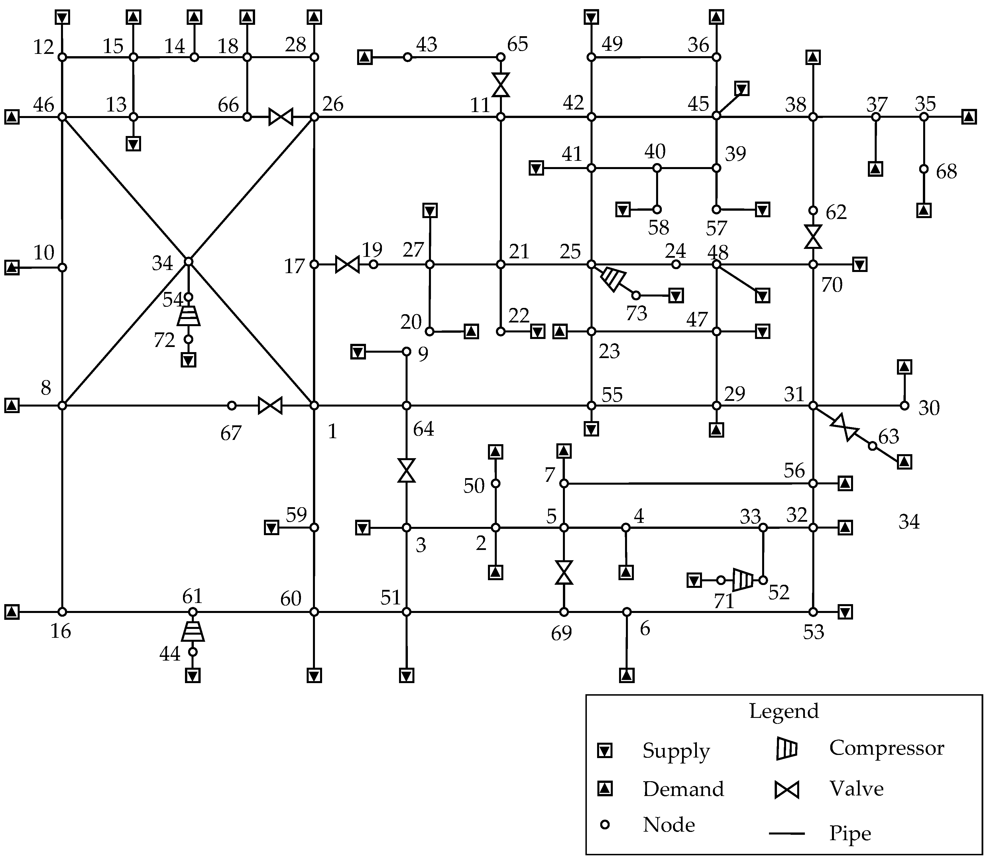
The complex pipeline is comprised of 84 pipelines, four compressors, eight valves, and 51 externals, and the structure of the complex pipeline network is shown in Figure 5 and detailed data are given in

Table 3. Pipeline data.

Pipeline	1	2	3	4	5	6	7	8	9	10	11	12	13	14
Starting node	64	3	5	51	5	69	5	67	8	9	46	15	13	66
Ending node	1	2	2	3	4	6	7	8	10	64	10	12	46	13
Length (km)	52	78	66	40	23	22	39	58	50	60	35	59	57	56
Diameter (mm)	325	325	325	219	325	219	325	273	457	168	273	355	273	219
Pipeline	15	16	17	18	19	20	21	22	23	24	25	26	27	28
Starting node	13	14	1	17	66	18	19	27	27	22	25	25	24	26
Ending node	15	15	17	26	18	14	27	20	21	21	21	23	25	28
Length (km)	60	63	20	46	36	75	41	33	33	42	78	83	45	135
Diameter (mm)	273	168	457	457	273	325	219	219	168	168	355	355	355	457
Pipeline	29	30	31	32	33	34	35	36	37	38	39	40	41	42
Starting node	55	31	31	32	32	53	52	8	37	38	45	45	39	40
Ending node	64	29	30	56	33	6	33	61	35	37	38	39	40	41
Length (km)	92	46	74	50	40	77	25	85	63	85	69	44	76	67
Diameter (mm)	457	457	355	508	508	219	508	426	426	426	426	426	219	355
Pipeline	43	44	45	46	47	48	49	50	51	52	53	54	55	56
Starting node	11	65	56	47	11	26	2	41	45	12	53	54	29	31
Ending node	26	43	7	48	21	34	50	42	42	46	32	34	55	56
Length (km)	115	46	74	53	63	86	63	72	142	93	80	53	102	50
Diameter (mm)	426	273	273	219	219	355	219	426	426	325	325	508	426	426
Pipeline	57	58	59	60	61	62	63	64	65	66	67	68	69	70
Starting node	57	58	59	60	61	35	69	1	31	8	16	61	60	38
Ending node	39	40	1	59	1	68	51	34	70	16	61	60	51	62
Length (km)	30	68	43	56	52	36	45	52	52	80	84	101	95	33
Diameter (mm)	168	325	273	273	325	355	273	355	355	273	273	426	426	325
Pipeline	71	72	73	74	75	76	77	78	79	80	81	82	83	84
Starting node	41	23	33	18	49	45	49	8	46	11	24	48	47	23
Ending node	25	55	4	28	42	36	36	34	34	42	48	70	29	47
Length (km)	68	42	42	68	52	50	43	52	59	66	49	63	76	53
Diameter (mm)	355	273	457	273	273	273	219	355	325	355	355	325	325	219

Note: Diameter in Table 3 is outside diameter.

,

Table 4. Compressor data.

Compressor	1	2	3	4
Starting point	71	72	73	74
Ending point	52	54	25	61

,

Table 5. Valve data.

Valve	1	2	3	4	5	6	7	8
Starting point	70	31	17	64	11	1	26	5
Ending point	62	63	19	3	65	67	66	69

and

Table 6. External data.

Externals	1	2	3	4	5	6	7	8	9	10	11	12	13
Adjacent node	37	53	45	47	48	56	51	3	49	71	70	13	12
Externals	14	15	16	17	18	19	20	21	22	23	24	25	26
Adjacent node	72	55	22	58	9	57	73	41	59	60	27	44	6
Externals	27	28	29	30	31	32	33	34	35	36	37	38	39
Adjacent node	7	8	23	46	28	20	50	4	16	29	38	43	30
Externals	40	41	42	43	44	45	46	47	48	49
Adjacent node	2	36	63	10	15	18	14	35	68	32

. All the pipelines are horizontal, with a roughness, thickness, and thermal conductivity of 0.02286 mm, 5 mm, and 0.0127 W/(m·K), respectively.

The components of natural gas are listed in

Table 7. Main components of natural gas.

Component	CH4	C2H4	C3H8	N2	CO2
Volume fraction (%)	97.07	0.17	0.02	0.71	2.03

. The standard pressure and temperature are 101.325 kPa and 20 °C, respectively. The Colebrook Equation is used as the friction Equation [35]. During simulation, the ambient temperature is maintained at 15 °C.

The initial pressure is 2.8 MPa, the initial volume flow rate is zero, and the initial temperature is 15 °C. After t = 0 h, the pressure of some externals is maintained, the volume flow rate of some externals increases suddenly, the compressors are started, and the valves are opened. During the simulation, the volume flow rate of some externals is constant, while the volume flow rate of other externals and the valve opening (FR) of valves are changed, shown as

Table 8. Constant boundary conditions - pressure of the external.

Externals	10	14	20	25	46	48
Pressure (MPa)	2.8	2.8	2.8	2.8	2.5	2.5

,

Table 9. Constant boundary conditions flow rate of the external (flow in).

Externals	1	2	3	5	6	7	8	9	11	12
Volume flow rate (104 Nm3/d)	−9	85	25	26	−100	44	15	36	55	68
Externals	15	16	17	18	19	21	22	23	24	27
Volume flow rate (104 Nm3/d)	25	15	18	14	2	14	21	56	12	-34
Externals	28	29	30	31	32	33	35	36	37	38
Volume flow rate (104 Nm3/d)	−142	−13	−150	−45	−13.7	−14	−35	−22	−13	−44
Externals	39	40	41	42	43	44	45	47	49
Volume flow rate (104 Nm3/d)	−21	−25	−50	−16	−56	−69.4	−63	−66	−85

and

Table 10. Changed boundary conditions.

	External 4	External 13	External 26	External 34	Valves 1-8
	Volume flow rate (104 Nm3/d)				FR
0 h ≤ t < 5 h	22	32	-80	-68	1.0
5 h ≤ t < 10 h	0	0	0	0	0.1
t ≥ 10 h	22	32	-80	-68	1.0

, respectively. It is assumed that: (1) all the compressors have the same performance curve as shown in Figure 6, the rated speed of the compressor is 6000 RPM, and the start time is 3 minutes; (2) all the valves are same, the flow coefficient of the valve in this paper is calculated by the Equation C_v = 200 − 200FR, and the travel time of the valve is one minute.

5.2. Comparison of Numerical Accuracy

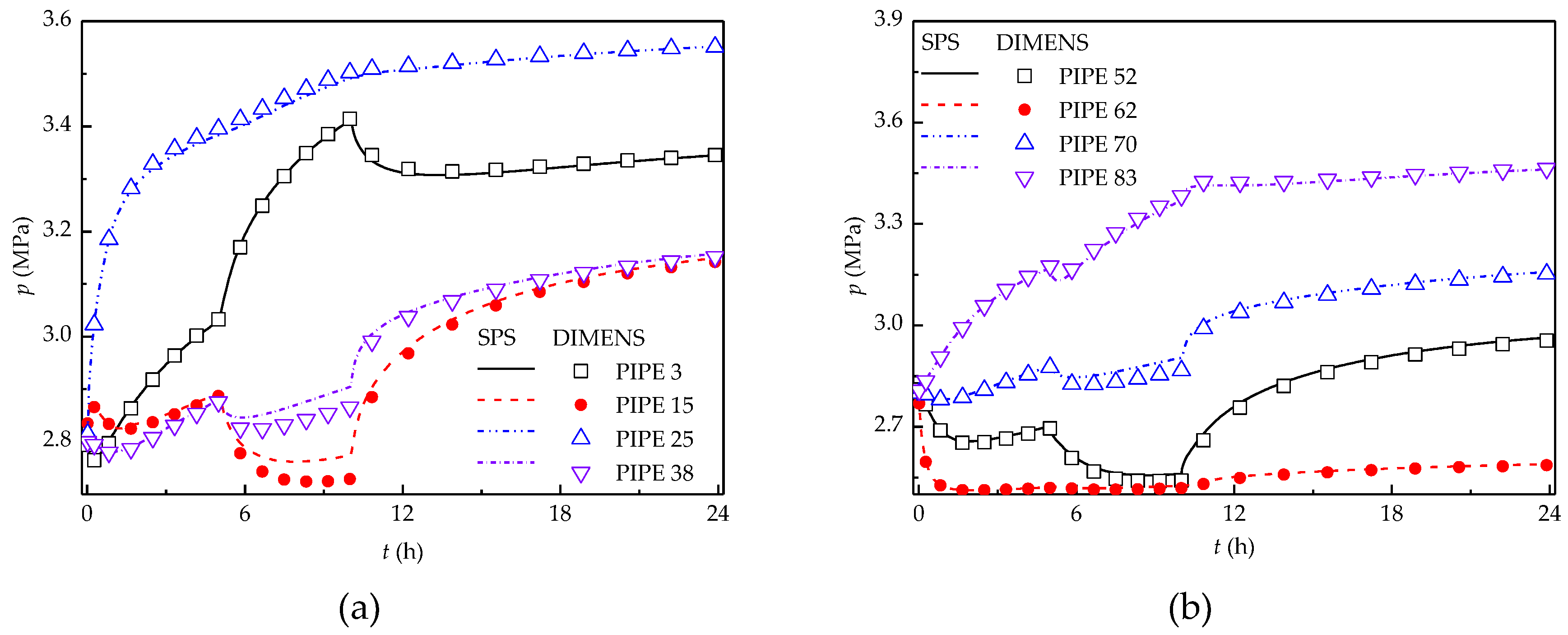
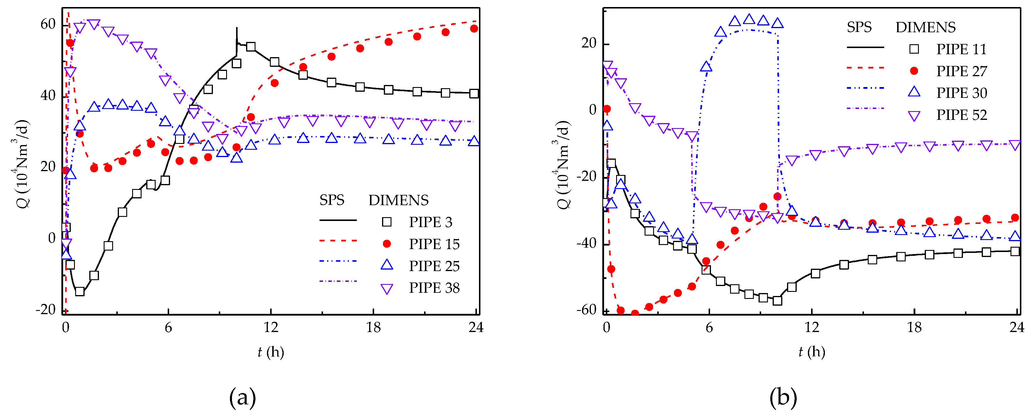
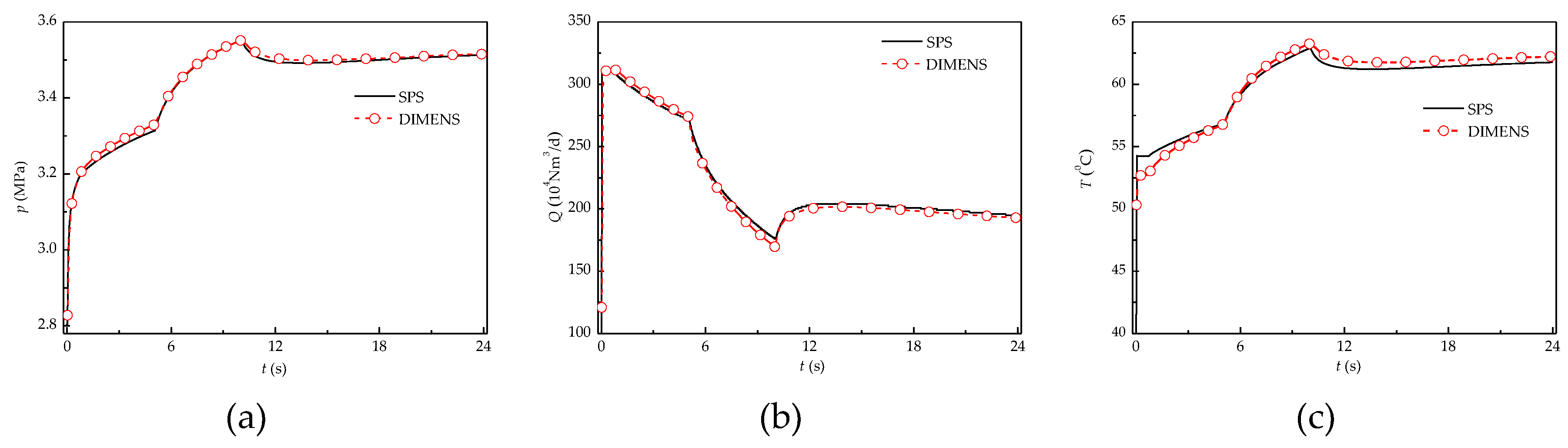
The case of the complex pipeline network is simulated by the DIMENS and SPS, respectively. The time step and spatial step are 10 s and 0.5 km, respectively. The pressure, volume flow rate, and temperature of the starting point of some pipelines during 0–10 h are shown in Figure 7, Figure 8 and Figure 9. The pressure, volume flow rate, and temperature of the compressor 1# are shown in Figure 10.

Figure 7, Figure 8 and Figure 9 show that the numerical solutions of flow simulation, such as pressure and flow rate, obtained by the DIMENS method, are in good agreement with those obtained by SPS. The results of these comparisons are the same as in previous literature [28]. This can validate the DIMENS method for flow equations of the complex pipeline network. In addition, it is clearly seen from Figure 9 that the difference between the temperature obtained by the DIMENS method and that obtained by SPS is very small. The maximum deviation of temperature of the two methods is less than 1 °C, which can be found at the starting point of pipe 63 at t = 6 h, as shown in Figure 9b. This is acceptable for practical engineering problems of natural gas pipeline transportation. That is to say, the DIMENS method is also accurate for the thermodynamic simulation. Additionally, the results of pressure, flow rate, and temperature of the compressor obtained by the DIMENS method are also in good agreement with those of SPS, as shown in Figure 10. This means that the complex start-up process of the compressor can be accurately simulated by the DIMENS method too. The above analysis shows that the DIMENS method has a high accuracy comparable to the accuracy of the SPS and can meet the requirements of practical engineering problems.

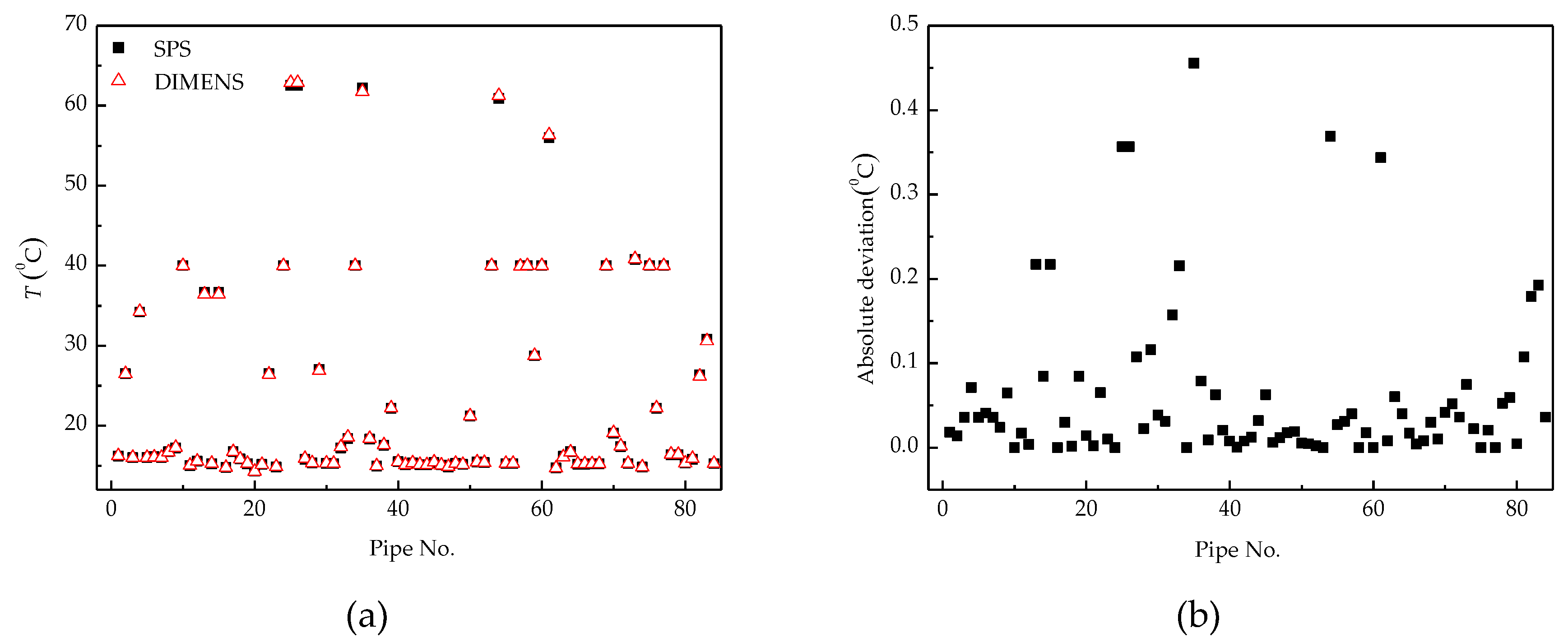
To further test the simulation accuracy of the DIMENS method, the results of the pipeline network at t = 24 h obtained by the DIMENS method and SPS are compared, as shown in Figure 11, Figure 12 and Figure 13.

From the comparison of the pressure of the connection nodes in Figure 11, it can be seen that the pressures obtained by the two methods are almost the same, and the maximum absolute and relative deviations of pressure are 0.015 MPa and 0.45%, respectively. From the comparison of the volume flow rate in Figure 12, the maximum absolute and relative deviations of the volume flow rate are 2.4 × 10⁴ Nm³/h and 3.5%, respectively. What is more, the maximum absolute deviation of temperature is less than 0.5 °C, as shown in Figure 13. It can be summarized that the deviation between the numerical solution calculated by the DIMENS method and SPS is sufficiently small. These analyses again imply that the calculation accuracy of the DIMENS method is comparable to that of SPS.

5.3. Comparison of Computational Efficiency

The number of discretized grid points of the pipeline network and the number of pipeline sections of the pipeline network are two main factors that can affect the efficiency of pipeline network simulation. Therefore, the computational speed of the DIMENS method proposed in this paper is examined from three aspects: (1) the number of discretized grid points; (2) the number of components; and (3) the number of discretized grid points and the number of components. The restart process of the complex pipeline network is simulated by both the DIMENS method and SPS, and the CPU times are recorded and compared. The time step is 10 s, and the simulation time is 1 day. The computations are carried out on a computer equipped with a 2.6 GHz Intel Xeon E5-2640 CPU with 64 GB RAM.

First, the topology of the pipeline network in Figure 5 is unchanged, while the pipelines are discretized by different spatial steps. The adaptability of the DIMENS method for the number of discretized grid points is studied. The CPU time is shown in Figure 14.

It can be seen from Figure 14 that the CPU time of the DIMENS method is less than that of the SPS. This means that the DIMENS method is more efficient than SPS. What is more, the CPU times of these two methods are both almost linear with the number of discretized points. This indicates that the DIMNES method and the SPS both have a strong adaptability to the increase of discretized points of the pipeline network. However, with the same number of discretized points, the CPU time of SPS is always longer than that of DIMENS method. The slope of the line of the DIMENS method in Figure 14 is 0.01, while that of SPS is 0.036. This is means that the efficiency of the DIMENS method is about 0.0036/0.01 = 3.6 times higher than that of the SPS as the number of discretized points is increasing. In other word, the DIMENS method is more efficient than SPS.

Second, the total number of discretized grid points is unchanged, while the number of components of the pipeline network is increased. The adaptability of the DIMENS method for the number of components is studied. The CPU time is shown in Figure 15.

It is clearly shown in Figure 15 that the CPU time of the DIMENS method is also less than that of the SPS. This means that the computational efficiency of the DIMENS method is high. What is more, the CPU time of the DIMENS method and that of the SPS are both linear with the number of components. The fit linear curve of SPS is y = 376 + 0.55x, and that of DIMENS is y = 31 + 0.59x. In other words, the gradients of the two lines are similar. Thus, the DIMNES method and the SPS are both not only well adapted to the increase of discrete points, but also to the increase of components. This indicates that the DIMNES method and the SPS both have a strong adaptability to the number of pipeline sections.

Last, the pipe network, as shown in Figure 5, is copied multiple times and connected to each other to form a larger network. The adaptability of the DIMENS method for the couple of grid points and components is studied. The CPU time is shown in Figure 16.

Figure 16 shows that the CPU time of the DIMENS method and that of the SPS are both linear with multiple network expansions. However, with the same multiple network expansions, the CPU time of SPS is always more than that of DIMENS method, and the slope of the line of the DIMENS method is smaller than that of SPS. That is to say, the CPU time of the DIMENS method is always less than that of SPS, and the DIMENS method would be more time-saving with the larger scale of the pipe network. This indicates that the DIMENS method is more efficient than SPS. It can be further seen that the fitted linear curve of SPS is y = 45 + 405x, while that of DIMENS is y = −56 + 187x. In other words, the slope of the line of the DIMENS method is about 187, while the slope of the line of SPS is about 405, which is over two times greater (405/187 = 2.16) than that of the DIMENS method. This means that the computing efficiency of the DIMENS method is over two times greater than that of SPS.

6. Conclusions and Future Work

In this paper, the DIMENS method has been extended to the flow and thermodynamic-coupled simulation of the complex pipeline network that includes pipelines and non-pipeline components. The simulation accuracy and efficiency of the present method have been investigated through an example of the complex pipeline network. The conclusions are as follows:

(1)

DIMES shows a very good agreement with SPS (differences below 3.5%). This accuracy can meet the requirements of practical engineering;

(2)

The CPU time of the DIMENS method is always less than that of SPS, and the computational speed of the DIMENS method is over two times higher than that of the SPS;

(3)

The DIMENS method has a strong adaptability to the scale of the pipeline network. The CPU time of the DIMNES method is linear with the size of the pipeline network.

In recent years, as a rapidly developing role in High Performance Computing (HPC), Graphic Processing Unit (GPU) computing has been becoming a research hotspot in many research fields. In order to maximize the GPU computing speed, the parallel granularity of the computational task should be fine enough. Thus, the algorithm should be highly parallel. In the DIMENS method, the pipelines in the network are parallel and the solution process of one pipeline is parallel too. This means that the parallel characteristic of the DIMENS method greatly matches the GPU. Therefore, to improve the computational speed further, it would be meaningful and worthwhile to study the GPU-accelerated simulation for large-scale natural gas pipeline networks in the future.

References

- Birol, F. Golden Rules for a Golden Age of Gas: World Energy Outlook Special Report on Unconventional Gas: Report. International Energy Agency. Available online: www.worldenergyoutlook.org/media/weowebsite/2012/goldenrules/WEO2012_GoldeGRulesReport.pdf (accessed on 22 October 2012).
- Turner, W.J.; Kwon, P.S.J.; Maguire, P.A. Evaluation of a gas pipeline simulation program. Math. Comput. Model. 1991, 15, 1–14. [Google Scholar] [CrossRef]
- Ouellette, L.; Hanks, H. Integrated simulation and SCADA to replay historical data for a local distribution company. In Proceedings of the PSIG Annual Meeting, Pipeline Simulation Interest Group, Tucson, AZ, USA, 15–17 October 1997. [Google Scholar]
- Hendriks, P.H.G.M.; Postvoll, W.; Mathiesen, M.; Spiers, R.P.; Siddorn, J. Improved capacity utilization by integrating real-time sea bottom temperature data. In Proceedings of the PSIG annual Meeting, Pipeline Simulation Interest Group, Williamsburg, VA, USA, 23–25 October 1995. [Google Scholar]
- Osiadacz, A. Simulation and Analysis of Gas Networks; E. & F.N. Spon Ltd.: London, UK, 1987; pp. 69–82. [Google Scholar]
- Helgaker, J.F.; Müller, B.; Ytrehus, T. Transient flow in natural gas pipelines using implicit finite difference schemes. J. Offshore Mech. Arct. Eng. 2014, 136, 031701. [Google Scholar] [CrossRef]
- Wang, H.; Liu, X.; Zhou, W. Transient flow simulation of municipal gas pipelines and networks using semi implicit finite volume method. Procedia Eng. 2011, 12, 217–223. [Google Scholar] [Green Version]
- Ebrahimzadeh, E.; Shahrak, M.N.; Bazooyar, B. Simulation of transient gas flow using the orthogonal collocation method. Chem. Eng. Res. Des. 2012, 90, 1701–1710. [Google Scholar] [CrossRef]
- Alamian, R.; Behbahani-Nejad, M.; Ghanbarzadeh, A. A state space model for transient flow simulation in natural gas pipelines. J. Nat. Gas Sci. Eng. 2012, 9, 51–59. [Google Scholar] [CrossRef]
- Behbahani-Nejad, M.; Shekari, Y. The accuracy and efficiency of a reduced-order model for transient flow analysis in gas pipelines. J. Pet. Sci. Eng. 2010, 73, 13–19. [Google Scholar] [CrossRef]
- Farzaneh-Gord, M.; Rahbari, H.R. Unsteady natural gas flow within pipeline network, an analytical approach. J. Nat. Gas Sci. Eng. 2016, 28, 397–409. [Google Scholar] [CrossRef]
- Pambour, K.A.; Bolado-Lavin, R.; Dijkema, G.P.J. An integrated transient model for simulating the operation of natural gas transport systems. J. Nat. Gas Sci. Eng. 2016, 28, 672–690. [Google Scholar] [CrossRef]
- Madoliat, R.; Khanmirza, E.; Moetamedzadeh, H.R. Transient simulation of gas pipeline networks using intelligent methods. J. Nat. Gas Sci. Eng. 2016, 29, 517–529. [Google Scholar] [CrossRef]
- Wang, J.; Wang, T.; Wang, J. Application of π equivalent circuit in mathematic modeling and simulation of gas pipeline. Appl. Mech. Mater. 2014, 496, 943–946. [Google Scholar] [CrossRef]
- Herrán-González, A.; Cruz, J.M.D.L.; De Andrés-Toro, B.; Risco-Martín, J.L. Modeling and Simulation of a Gas Distribution Pipeline Network. Appl. Math. Model. 2009, 33, 1584–1600. [Google Scholar] [CrossRef]
- Thorley, A.R.D.; Tiley, C.H. Unsteady and transient flow of compressible fluids in pipelines—A review of theoretical and some experimental studies. Int. J. Heat Fluid Flow 1987, 8, 3–15. [Google Scholar] [CrossRef]
- Kiuchi, T.T.; Izumi, H.H.; Huke, T.T. An operation support system of large city gas networks based on fluid transient model. J. Energy Resour. Technol. 1995, 117, 324–328. [Google Scholar] [CrossRef]
- Kiuchi, T. An implicit method for transient gas flows in pipe networks. Int. J. Heat Fluid Flow 1994, 15, 378–383. [Google Scholar] [CrossRef]
- Wylie, E.B.; Stoner, M.A.; Streeter, V.L. Network: System transient calculations by implicit method. Soc. Pet. Eng. J. 1971, 11, 356–362. [Google Scholar] [CrossRef]
- Li, Y.; Yao, G. Design and Operation of Gas Pipeline; China University of Petroleum Press: Beijing, China, 2009; pp. 19–26. (In Chinese) [Google Scholar]
- Abbaspour, M.; Chapman, K.S. Non-isothermal transient flow in natural gas pipeline. J. Appl. Mech. 2008, 75, 031018. [Google Scholar] [CrossRef]
- Luskin, M. An approximation procedure for non-symmetric, nonlinear hyperbolic systems with integral boundary conditions. Siam J. Numer. Anal. 1979, 16, 145–164. [Google Scholar] [CrossRef]
- Zheng, J.G.; Chen, G.Q.; Song, F.; Ai, M.Y.; Zhao, J.L. Research on simulation model and solving technology of large scale gas pipe network. J. Syst. Simul. 2012, 14, 133. (In Chinese) [Google Scholar]
- Barley, J. Thermal decoupling: An investigation. In Proceedings of the PSIG annual Meeting, Pipeline Simulation Interest Group, Santa Fe, NM, USA, 16–19 April 2012. [Google Scholar]
- Helgaker, J.F.; Ytrehus, T. Coupling between continuity/momentum and energy Equation in 1D gas flow. Energy Procedia 2012, 26, 82–89. [Google Scholar] [CrossRef]
- Wang, P.; Yu, B.; Deng, Y.; Zhao, Y. Comparison study on the accuracy and efficiency of the four forms of hydraulic Equations of a natural gas pipeline based on linearized solution. J. Nat. Gas Sci. Eng. 2015, 22, 235–244. [Google Scholar] [CrossRef]
- Stoner, M.A. Sensitivity analysis applied to a steady-state model of natural gas transportation systems. Soc. Pet. Eng. J. 1972, 12, 115–125. [Google Scholar] [CrossRef]
- Wang, P.; Yu, B.; Han, D.; Sun, D. Fast method for the hydraulic simulation of natural gas pipeline networks based on the divide-and-conquer approach. J. Nat. Gas Sci. Eng. 2018, 50, 55–63. [Google Scholar] [CrossRef]
- Keenan, P.T. Collation and upwinding for thermal flow in pipelines: The linearized case. Int. J. Numer. Methods Fluids 1996, 22, 835–849. [Google Scholar] [CrossRef]
- Osiadacz, A.J.; Chaczykowski, M. Comparison of isothermal and non-isothermal pipeline gas flow models. Chem. Eng. J. 2001, 81, 41–51. [Google Scholar] [CrossRef]
- Wang, P.; Yu, B.; Han, D.; Li, J.; Sun, D.; Xiang, Y.; Wang, L. Adaptive implicit finite difference method for natural gas pipeline transient flow. Oil Gas Sci. Technol. Rev. D’ifp Energ. Nouv. 2018, 73, 21. [Google Scholar] [CrossRef]
- Chaczykowski, M. Sensitivity of Pipeline Gas Flow Model to the Selection of the Equation of State. Chem. Eng. Res. Des. 2009, 87, 1596–1603. [Google Scholar] [CrossRef]
- Benedict, M.; Webb, G.B.; Rubin, L.C. An empirical Equation for thermodynamic properties of light hydrocarbons and their mixtures I. Methane, ethane, propane and n-butane. J. Chem. Phys. 1940, 8, 334–345. [Google Scholar] [CrossRef]
- Scott, L.R. Numerical Analysis, 2nd ed.; Princeton University Press: Oxford, MS, USA, 2016; pp. 53–64, 145–149. [Google Scholar]
- Colebrook, C.F. Turbulent flow in pipes with particular reference to the transition region between the smooth and rough pipe laws. J. Inst. Civ. Eng. 1939, 11, 133–156. [Google Scholar] [CrossRef]
Figure 1.
Grids of the pipeline
Figure 2.
The decoupled strategy.
Figure 3.
Divide-and-conquer approach for the natural gas pipeline network.
Figure 4.
Procedure of the DIMENS method for the pipeline network.
Figure 5.
The schematic diagram of the topology structure of the complex pipeline network.
Figure 6.
The performance curve of the compressor.
Figure 7.
Pressure of the starting point of some pipelines: (a) Pipe 3, 15, 25, and 38; (b) Pipe 52, 62, 70, and 83.
Figure 8.
Volume flow rate of the starting point of some pipelines: (a) Pipe 1, 62, 72, and 81; (b) Pipe 11, 27, 30, and 52.
Figure 9.
Temperature of the starting point of some pipelines: (a) Pipe 9, 17, 36, and 78; (b) Pipe 27, 45, 56, and 63.
Figure 10.
Pressure, flow rate, and temperature at the outlet of the 1#compressor outlet: (a) Pressure; (b) flow rate; (c) temperature.
Figure 11.
Comparison of pressure at the connection node: (a) Pressure value; (b) deviation.
Figure 12.
Comparison of flow rate of pipelines: (a) Flow rate value; (b) deviation.
Figure 13.
Comparison of temperature at the start and end nodes of pipelines: (a) Temperature value at the start node; (b) deviation at the start node; (c) temperature value at end node; (d) deviation at the end node.
Figure 14.
Change of CPU time with the number of discretized grid points.
Figure 15.
Change of computing time with the number of pipeline sections.
Figure 16.
Change of computing time with multiple network expansions.