Multi-Objective Optimization of Energy Saving Control for Air Conditioning System in Data Center

Abstract

A multi-objective optimization scheme is proposed to save energy for a data center air conditioning system (ACS). Since the air handling units (AHU) and chillers are the most energy consuming facilities, the proposed energy saving control scheme aims to maximize the saved energy for these two facilities. However, the rack intake air temperature tends to increase if the energy saving control scheme applied to AHU and chillers is conducted inappropriately. Both ACS energy consumption and rack intake air temperature stabilization are set as two objectives for multi-objective optimization. The non-dominated sorting genetic algorithm II (NSGA-II) is utilized to solve the multi-objective optimization problem. In order for the NSGA-II to evaluate fitness functions that are both the ACS total power consumption and AHU outlet cold air temperature deviations from a specified range, neural network models are utilized. Feedforward neural networks are utilized to learn the power consumption models for both chillers and AHUs as well as the AHU outlet cold air temperature based on the recorded data collected in the field. The effectiveness and efficiency of the proposed energy saving control scheme is verified through practical experiments conducted on a campus data center ACS.

1. Introduction

Following the increasing demand for Internet of Things (IOT), big data, cloud computing, artificial intelligence, etc., more information technology (IT) equipment such as servers, data storage, and network communication devices as well as uninterruptible power systems have been placed into data centers. In order to save limited data center space, the IT equipment is stacked into rows of racks inside cabinets. A great deal of heat exhaust is generated as these IT equipment and facilities operate. However, constant low temperature and humidity are required in the data center so that the IT equipment and associated facilities can operate under normal conditions [1,2]. A delicate air conditioning system (ACS) is installed in the data center to remove heat exhaust from every cabinet rack containing IT equipment. In addition to heat removing from the racks, maintaining constant indoor temperature and humidity in the data center is also a major function of ACS. A great deal of power consumption is required in order for the ACS to provide these functions. The average power consumption of ACS usually takes up as high as 40% of the total power [3,4]. The data center not only runs 24 h a day, 7 days a week all year round, but it is also energy intensive with typical power densities of 538–2153 W/m² and sometimes can be as high as 10 kW/m² [5]. It was reported in [6] that data centers in the U.S. consumed an estimated 70 billion kWh, representing 1.8% of the total U.S. electricity consumption. Over the past decade, saving energy consumption has become an important technological effort for sustainable development of data centers. Since a big portion of data center power consumption is due to ACS, various effective energy saving techniques for ACS have been proposed by engineers and scientists in the past several decades.

There are guidelines and standards for building energy-efficient data centers [7]. In [8], the power usage effectiveness (PUE) was proposed as the metric evaluating power utilization efficiency for data centers. Recently, PUE has become a prevailing international standard comparing power usage effectiveness among different data centers. Different levels of PUE for data center have also been proposed [9,10]. PUE is defined as the ratio of total power consumption in a data center to the power consumption of the IT equipment in that data center. Since ACS power consumption could occupy as high as 40% of the total data center power consumption, minimizing ACS power consumption is an effective approach to minimizing PUE. Minimizing PUE has become a big challenge for scientists and engineers in this area. The ACS is thus the main target for PUE minimization due to its high power consumption. The ACS consists mainly of a chilled water loop and airflow loop. Both loops are greatly affected by each other. The greatest energy-consuming facilities in chilled water loop and airflow loop are the chiller and air handling unit (AHU), respectively. Chillers and AHUs are thus the primary targets conducting energy saving control techniques proposed in this paper to minimize PUE of data center. However, if the energy saving control scheme applied to ACS saves too much energy, the rack intake temperature may rise and affect heat exhaust removal for servers. The optimization is thus designed to maintain the rack intake temperature within a specified range in addition to saving energy for both chillers and AHUs. The metric called rack cooling index (RCI) [11,12] is utilized to evaluate the performance of rack intake temperature control for data center. The RCI is ideally maximized if the best control of rack intake temperature control is achieved. A multi-objective optimization approach is proposed in this paper minimizing PUE and maximizing RCI simultaneously. For practical control of ACS in data center, variants for minimizing PUE and maximizing RCI are developed for multi-objective optimization. It will be shown in the paper that the minimization of PUE is achieved by power consumption minimization of chillers and AHUs. Similarly, it is impractical to monitor and control intake temperature of every rack inside cabinets. Since AHU outlet cold air temperature directly influences the intake temperature of every rack, the maximization of RCI is achieved by optimal control of AHU outlet cold air temperature.

Airflow management imposes a pronounced effect on energy saving of ACS. The airflow cooling systems in the data center can be categorized as long distance and short distance [13]. Research on improving long-distance airflow management for ACS is as follows. The chilled airflow is driven by AHU to the IT equipment piled up on racks through a longer distance for a long-distance cooling system. The airflow cooled down at AHU is sent to racks mitigating the heat generated by the IT equipment through cold aisles. The heated airflow is then circulated back to the AHU through hot aisles. In order to avoid or reduce hot airflow recirculation, short-distance cooling systems are designed where the airflow is circulated close by or among racks. Long-distance cooling systems are generally more commonly used, and are mainly the focus of this paper. There are several ways to improve long-distance airflow cooling. The flowrate uniformity is affected by frictional resistance, which can be improved by increasing the plenum depth [14]. The plenum depth is recommended to be 600 mm and 1080 mm, respectively, in [15,16]. The cold air is sent to computer racks through perforated tiles. Therefore, perforated tiles and a raised floor are essential parts of cold aisles. It is obvious that the cold air flowrate can be improved if porous tiles are used on the raised floor. However, it was found in [17] that flow rate uniformity is affected if the tile porosity is increased above certain limits. The guidelines in selecting perforated tiles for data centers were recommended in [18]. It was shown in [19,20] that as the pore size is reduced from 6.35 mm to 3.18 mm, the flow field was influenced to an extent that cannot be overlooked. Another way to enhance the airflow uniformity is to install induced bypass fans in the plenum. It was shown in [21] that the energy consumption can be reduced by as much as 60% if the bypass fans along with the proposed optimized tiles are utilized in cold aisles. The fans in AHU can operate at lower running speed if the bypass fans are installed. As much as 52% power consumption can be saved in the cooling system with lower running fans [22,23]. A mathematical model was proposed in [24,25] for numerical performance evaluation on fan-assisted perforations in data centers. Apart from the mathematical model, bypass fans integrated with modified perforated tiles were proposed in [26] to experimentally study the effect on temperature and airflow distribution improvement.

Different from the aforementioned long-distance airflow management techniques that mainly focus on the airflow from AHU through plenum to IT equipment cabinets, the short-distance airflow management is conducted among racks inside a cabinet. The rack-level heat exchangers were installed beside servers and studied in [27,28] to further improve PUE. The modeling and transient response of a rack-level heat exchanger were studied in [27] while the energy-saving improvement compared with conventional long-distance cooling system were analyzed in [28]. Heat pipe technology has lately been applied to data center short-distance cooling systems. The airflow is drawn into the rack cabinet by fans and the heat exhaust in the cabinet is taken away by the heat pipes. A thermal bus system composed of thermosyphon was proposed and analyzed in [29], showing that the significant thermal resistance reduction was achieved. A novel system integrating two hybrid cooling systems combining dew-point evaporative coolers with heat pipes for data center was installed and investigated in [30]. It was shown in [30] that the coefficient of performance (COP) of the hybrid cooling system was as high as 34, leading to annual energy savings of nearly 90% compared with conventional vapor compression cooling system.

There are not too many research articles that have investigated energy saving approaches for ACS other than airflow management in data centers. The outside air, direct wet-side evaporative heat exchangers, and indirect wet-side chilled water loops for cooling were proposed to improve ACS energy efficiency in data centers [31]. An indirect-heat-exchanger-based water-side economizer system was installed in [32] to improve ACS energy efficiency. It was shown in [32] that the proposed water-side economizer could achieve a maximum energy performance improvement of about 16.6% over the reference base cooling system. Another easy and straightforward approach to improve data center energy efficiency is to adjust the indoor temperature setting. The impact of raising data center temperature on the servers was investigated in [33,34]. In fact, raising the supply air temperature in data centers does not necessarily reduce the energy consumption because the airflow rate might be increased leading to increasing AHU energy consumption. In [35], an integrated water side economizer was proposed to optimize the energy performance by adjusting the air temperature and the airflow rate settings through simulations using the software TRNSYS. A mathematical model calculating energy consumption in data centers at different temperature settings was proposed in [36]. The energy consumptions calculated using the proposed model were compared with the measured data and achieved satisfied results.

Apart from approaches improving ACS energy efficiency in data centers on either the air or water side, some intelligent control as well as multi-variable control schemes were applied to heating, ventilation, and air conditioning (HVAC) systems that can also be applied to data center ACS. Various complex controllers were designed to control AHU in [37,38,39,40] and chillers in [41,42,43] in order to improve ACS energy efficiency for buildings. However, not too many researches were found applying those complex controllers for HVAC to the ACSs in data centers. Since the multi-objective optimization problem to be solved in this paper is a non-convex and nonlinear problem, random optimization approaches such as simulated annealing [44], genetic algorithm (GA) [45], particle-swarm optimization (PSO) [46,47], and evolutionary algorithm (EA) [48] are commonly utilized. The non-dominated sorting genetic algorithm II (NSGA-II) [49] is applied in this paper for multi-objective optimization. The technical novelty and main contribution of this paper are summarized as follows:

• A multi-objective optimization approach that simultaneously optimizes power consumption of chillers and AHUs as well as AHU outlet cold air temperature for the ACS in data center is introduced. To the best of our knowledge, no similar works addressing this issue have ever been proposed in the literature.
• An optimal energy saving control technique for the ACS in data center is proposed so that the most commonly used international standards PUE and RCI are both optimized.
• In order for NSGA-II to evaluate the fitness value corresponding to every chromosome, feedforward neural network (FNN) models are constructed based on recorded data collected from the field. NSGA-II has been successfully applied to on-line calculation along with constructed neural network models.
• The proposed NSGA-II based multi-objective optimization approach has been practically applied to the ACS of a campus data center and the average energy saving ratios are 23.4% and 19.6% for a typical winter and summer day, respectively.

This paper is structured as follows. The problem to be solved and the data center ACS are introduced in Section 2. Section 3 defines the multi-objective optimization model. The multi-objective optimization approach to be utilized in this paper, i.e., NSGA-II is described in Section 4. Along with NSGA-II, the models including chillers, AHUs, and the prediction model for the AHU outlet cold air temperature are constructed using FNN, which is also introduced in Section 4. The experiments verifying the effectiveness and efficiency of FNN modeling as well as the performance of energy saving control are shown in Section 5. Conclusions are made in Section 6.

2. Problem Statement and Data Center Air Conditioning System

The most energy-consuming facilities in the data center ACS are mainly AHUs and chillers. The energy saving control for the ACS thus aims to save energy for these two main facilities. It is shown in Figure 1 that the hot and cold air aisle configuration is used in the data center. The cold air is driven by the AHU through the plenums under the floor. The hot air exhausted from the IT equipment cabinets is circulated through hot air plenums above the data center ceiling back to the AHUs. The hot air returned to the AHUs is cooled through the chilled water pumped from the chillers to the AHUs. The IT equipment cabinets are lined up in alternating rows with cold air intakes facing one side and hot air exhausts facing the other. The cold/hot air circulation in the data center depends on the fan running speed in the AHU, while the cooling temperature of the returned hot air depends on the chilled water temperature. Therefore, the energy saving control for the data center ACS relies on the control of AHU fans and the output chilled water temperature from the chillers.

It is straightforward to reduce AHUs and chiller power consumption to save data center energy. However, the data center is an environment sensitive to temperature changes. It is easy to increase rack intake air temperature with inappropriate energy saving control schemes applied to AHUs and chillers. A real-time multi-objective optimization approach is to be implemented in an energy saving controller as shown in Figure 1. This approach simultaneously reduces ACS energy consumption and stabilizes the intake air temperature at every rack. Note that the intake temperature at every rack is directly influenced by the AHU cold air outlet temperature.

A commonly used metric PUE [7,8,9] for measuring data center energy efficiency is adopted in this paper that shows energy saving effectiveness. PUE is defined as the ratio of total energy consumed by all facilities in the data center to the energy consumed by the servers and other computing facilities. Denote $P_i$ as the power consumption of the i-th facility in the data center, $P_{AC}$ as the ACS power consumption and $P_{IT}$ as the power consumption due to all IT equipment, then

$$PUE=\frac{{\displaystyle \sum _i{P}_i}}{P_{IT}}=\frac{P_{AC}+{\displaystyle \sum _{i,i\ne AC}{P}_i}}{P_{IT}}.$$

(1)

The energy saving control scheme focuses mainly on reducing chiller and AHU power consumption leading to reducing $P_{AC}$ and thus reducing PUE according to Equation (1). Therefore, PUE is a suitable metric to measure the energy saving effectiveness in this paper.

Let N be the total number of intakes in all servers, $T_{\max \text{-}all}$ and $T_{\min \text{-}all}$ be the maximum and minimum allowable temperature, $T_{\max \text{-}rec}$ and $T_{\min \text{-}rec}$ be the maximum and minimum recommended temperature, and $T_i$ be the average temperature at the i-th intake. According to [11], RCI_HI and RCI_LO are respectively defined as:

$$RC{I}_{HI}=(1-\frac{{\displaystyle \sum _i{\left(T_i-T_{\max \text{-}rec}\right)|}_{T_i>T_{\max \text{-}rec}}}}{N\left(T_{\max \text{-}all}-T_{\max \text{-}rec}\right)})100\%;$$

(2)

$$RC{I}_{LO}=(1-\frac{{\displaystyle \sum _i{\left(T_{\min \text{-}rec}-T_i\right)|}_{T_i<T_{\min -rec}}}}{N\left(T_{\min -rec}-T_{\min -all}\right)})100\%.$$

(3)

RCI_HI and RCI_LO are metrics measuring intakes being over-temperature and under-temperature, respectively. It is reasonable to expect that most of RCI_LO are 100% because ACS energy savings may lead to the intake temperature increasing instead of decreasing. It is essential for the data center energy saving control to find an optimal compromise between saving energy and not affecting the rack intake temperature. Therefore, both PUE and RCI are utilized as objectives for the multi-objective optimization approach proposed in this paper.

3. Multi-Objective Optimization

The most straightforward and easiest way to control chiller power consumption is to control the chilled water outlet temperature $T_{chwo}(•)$ that directly affects the AHU outlet cold air temperature $T_f(•)$. Similarly, the AHU power consumption can be controlled by controlling AHU fans running speed $v_f(•)$. Assume that the running speed $v_f(•)$ of AHU fans is controlled using variable frequency drives that can be controlled through an inverter. Denote $T_{chwo}^L$ and $T_{chwo}^H$ as the lower and higher limit of the chilled water outlet temperature $T_{chwo}$; $v_f^L$ and $v_f^H$ as the lower and higher limit of the AHU fans running speed. The proposed energy saving control scheme searches for the optimal settings $T_{chwo}^{*}\left(k\right)$ and $v_f^{*}\left(k\right)$ at every k-th time step using the multi-objective optimization approach to simultaneously minimize PUE(k) and maximize both RCI_HI(k) and RCI_LO(k), i.e.,

$$\left(T_{chwo}^{*}\left(k\right),v_f^{*}\left(k\right)\right)=arg\underset{T_{chwo}\left(k\right)}{min}\underset{v_f\left(k\right)}{max}\left(PUE\left(k\right),RC{I}_{HI}\left(k\right),RC{I}_{LO}\left(k\right)\right).$$

(4)

subject to

$$T_{chwo}^L\le T_{chwo}\left(k\right)\le T_{chwo}^H;$$

(5)

$$v_f^L\le v_f\left(k\right)\le v_f^U.$$

(6)

Denote $P_{ch}\left(k\right)$ and $P_{AHU}\left(k\right)$ as the power consumption of the chiller and AHU, respectively, at the k-th time step. Most of the ACS power consumption is due to the power consumptions of both the chillers and AHUs. Therefore,

$$P_{AC}\left(k\right)\approx P_{ch}\left(k\right)+P_{AHU}\left(k\right).$$

(7)

Since the optimization variables $T_{chwo}\left(k\right)$ and $v_f\left(k\right)$ in (4) directly affect both $P_{ch}\left(k\right)$ and $P_{AHU}\left(k\right)$, the minimization of PUE(k) is practically achieved through the minimization of P_AC(k) according to Equations (1) and (7).

In parallel with minimizing $P_{AC}\left(k\right)$, every rack intake temperature needs to be maintained within a preset range satisfying both RCI_HI and RCI_LO, respectively, in Equations (2) and (3), i.e., within the range between maximum and minimum recommended temperature. For both the implementation convenience and installation cost, temperature sensors are not installed at every rack air intake. Referring to Figure 1, all the rack intake temperatures depend on the AHU outlet cold air temperature $T_f\left(k\right)$. Therefore, the following assumption can be made for practical engineering consideration:

$$T_i\left(k\right)\approx T_f\left(k\right),i=1\dots N.$$

(8)

Referring to Equations (2) and (7), RCI_HI(k) is maximized if both $T_{chwo}\left(k\right)$ and $v_f\left(k\right)$ are controlled so that $T_f\left(k\right)\le T_{\max \text{-}rec}$. Similarly, RCI_LO(k) is maximized if both $T_{chwo}\left(k\right)$ and $v_f\left(k\right)$ are controlled so that $T_{\min \text{-}rec}\le T_f\left(k\right)$ according to Equations (3) and (7). In other words, both RCI_HI(k) and RCI_LO(k) are maximized if the ACS is controlled by adjusting $T_{chwo}\left(k\right)$ and $v_f\left(k\right)$ so that

$$T_{\min \text{-}rec}\le T_f\left(k\right)\le T_{\max \text{-}rec}.$$

(9)

However, both $T_{\min \text{-}rec}$ and $T_{\max \text{-}rec}$ are recommended by ASHRAE [11], satisfying every data center in different regions with different climates. They are less strict, allowing greater flexibility suitable for as many data centers as possible. In order to have better temperature control performance, stricter lower and upper bounds $T_f^L$ and $T_f^U$ for $T_f\left(k\right)$ are given where $T_{\min \text{-}rec}<T_f^L$ and $T_f^U<T_{\max \text{-}rec}$ so that $T_f\left(k\right)$ is controlled within a smaller range. Therefore,

$$T_{\min \text{-}rec}<T_f^L\le T_f\left(k\right)\le T_f^U<T_{\max \text{-}rect}.$$

(10)

Denote the temperature difference $T_d(•)$ as:

$$T_d\left(k\right)=\max \left(0,\left(T_f^L-T_f\left(k\right)\right)\right)+\max \left(0,\left(T_f\left(k\right)-T_f^U\right)\right).$$

(11)

Therefore, the maximization of both RCI_HI(k) and RCI_LO(k) is achieved and even improved by the minimization of $T_d\left(k\right)$ in Equation (11). The multi-objective optimization min-max in Equation (4) is thus transformed into simultaneous minimization of $P_{AC}\left(k\right)$ in (7) and $T_d\left(k\right)$ in (11). In other words, the multi-objective optimization in (4) is replaced by the following multi-objective optimization:

$$\left(T_{chwo}^{*}\left(k\right),v_f^{*}\left(k\right)\right)=\underset{T_{chwo}\left(k\right),v_f\left(k\right)}{argmin}\left(P_{AC}\left(k\right),T_d\left(k\right)\right)$$

(12)

with the same constraints in (5) and (6).

The multi-objective optimization in Equation (12) with the constraints in (5) and (6) is calculated by the energy saving controller as shown in Figure 1. Most chillers have interfaces allowing remote setting for chilled water outlet temperature $T_{chwo}^{}\left(k\right)$. Similarly, most AHUs also have interfaces that allow remotely setting AHU fan running speed $v_f\left(k\right)$. Referring to Figure 1, the energy saving controller is designed to conduct the remote setting through the most commonly used RS-485 network. Other wired or wireless networks such as Ethernet, Wifi, Zigbee, etc., can also be used to replace RS-485 network.

4. NSGA-II and Neural Network Modeling

NSGA-II is utilized to implement the multi-objective optimization in Equation (12) with constraints in (5) and (6). Both the optimization variables $T_{chwo}^{}\left(k\right)$ and $v_f\left(k\right)$ are parameterized in the chromosome in real numbers. Both objective functions $P_{AC}\left(k\right)$ and $T_d\left(k\right)$ in (7) and (11), respectively, are utilized as the fitness functions. The crossover and mutation operators in NSGA-II are the same as the ones in regular genetic algorithm (GA). The Pareto-optimal solutions are searched from the best non-dominated solutions in every generation based on the fitness value of every chromosome. However, it is not possible to practically measure both $P_{ch}\left(k\right)$ and $P_{AHU}\left(k\right)$ and then calculate $P_{AC}\left(k\right)$ corresponding to different optimization variables $T_{chwo}^{}\left(k\right)$ and $v_f\left(k\right)$ encoded in the chromosomes for NSGA-II on-line learning. The practical difficulty mainly comes from the fact that it usually takes a few minutes to more than half hour for the ACS to respond to both settings $T_{chwo}^{}\left(k\right)$ and $v_f\left(k\right)$, and finally to stabilize the entire system in order to measure the steady power consumption $P_{ch}\left(k\right)$ and $P_{AHU}\left(k\right)$, respectively for every chromosome. It is therefore not possible for the NSGA-II to perform on-line optimization of $T_{chwo}^{}\left(k\right)$ and $v_f\left(k\right)$ if the fitness value corresponding to every chromosome is to be practically measured from the ACS. Moreover, it will cause ACS mechanical impairment if both settings $T_{chwo}^{}\left(k\right)$ and $v_f\left(k\right)$ are changed so often, corresponding to every different optimization variable encoded in every chromosome of gene pool during the learning process of NSGA-II. Similarly, it is not possible to measure the AHU outlet cold air temperature $T_f\left(k\right)$ and then calculate $T_d\left(k\right)$ due to the same practical difficulty. In order to overcome this difficulty, an FNN-based model is learned a priori based on the recorded data measured in the field for $P_{ch}\left(k\right)$, $P_{AHU}\left(k\right)$, and $T_f\left(k\right)$, respectively so that each of these three variables can be estimated corresponding to different sets of optimization variables encoded in the chromosome as well as some variables measured on-line.

Denote ${\rho }_f$ as the flow rate of chilled water, $c_w$ as the specific heat capacity of water, the chilled water inlet temperature of chiller as $T_{chwi}\left(k\right)$. The cooling capacity Q of a chiller is calculated as:

$$Q\left(k\right)={\rho }_f{c}_w\left(T_{chwi}\left(k\right)-T_{chwo}\left(k\right)\right).$$

(13)

Referring to Equation (13), $P_{ch}\left(k\right)$ directly depends on the value of $\left(T_{chwi}\left(k\right)-T_{chwo}\left(k\right)\right)$ according to (13). $P_{ch}\left(k\right)$ can be expressed as a function of $\left(T_{chwi}\left(k\right)-T_{chwo}\left(k\right)\right)$. Denote this function as ${\Gamma }_{ch}$ which is to be learned and modeled by an FNN, $P_{ch}\left(k\right)$ can be expressed in association with ${\Gamma }_{ch}$ as:

$$P_{ch}\left(k\right)={\Gamma }_{ch}\left(T_{chwi}\left(k\right)-T_{chwo}\left(k\right)\right).$$

(14)

The function ${\Gamma }_{ch}$ is implemented as a 1 × 10 × 10 × 1 FNN with 1 input, 1 output, and 2 hidden layers with 10 neurons per layer. Back propagation is utilized as the learning approach.

The running speed of AHU fans $v_f\left(k\right)$ is usually adjusted through a PWM controller. Similar to the model for the chiller, the relationship between $P_{AHU}\left(k\right)$ and $v_f\left(k\right)$ can also be learned and modeled by an FNN. Denote ${\Gamma }_f$ as the function modeling this relationship, $P_{AHU}\left(k\right)$ can be expressed as:

$$P_{AHU}\left(k\right)={\Gamma }_f\left(v_f\left(k\right)\right).$$

(15)

The function ${\Gamma }_f$ is implemented as a 1 × 10 × 1 FNN with 1 input, 1 output, and 1 hidden layer with 10 neurons.

As for calculating the second objective $T_d\left(k\right)$ in Equation (11), a model estimating AHU outlet cold air temperature $T_f\left(k\right)$ is essential. Different from the models for $P_{ch}\left(k\right)$ and $P_f\left(k\right)$, note that any changes in the inputs for these two models ${\Gamma }_{ch}$ and ${\Gamma }_f$ are directly reflected to the outputs $P_{ch}$ and $P_f$, respectively, without time delay because the Chiller and AHU power consumptions vary with the input settings right away. However, it takes time for the AHU outlet cold air temperature $T_f$ to change because long distance airflow cooling system is targeted for control and $T_f$ is the temperature of the long distance airflow loop. Moreover, any changes $T_f$ are also related to the temperatures in previous time steps. It is assumed in this paper that predicted signal $T_f\left(k+1\right)$ are related to the temperatures in previous two time steps, i.e., $T_f\left(k\right)$ and $T_f\left(k-1\right)$. Although a data center is a closed environment, $T_f\left(k\right)$ is still affected by the outdoor temperature because the air-cooling chillers are installed outdoors. Therefore, $T_f\left(k\right)$ also depends on the outdoor temperature $T_o\left(k\right)$ which can be measured by a temperature sensor installed outdoors. Finally, both optimization variables $T_{chwo}\left(k\right)$ and $v_f\left(k\right)$ determined at every k-th time step also affect $T_f\left(k\right)$. Similar to previous modeling approaches, denote ${\Gamma }_{tmp}$ as a function modeling the relationship between $T_f\left(k+1\right)$ and other elements including $T_f\left(k\right)$, $T_f\left(k-1\right)$, $T_o\left(k\right)$, $T_{chwo}\left(k\right)$ and $v_f\left(k\right)$. Therefore,

$$T_f\left(k+1\right)={\Gamma }_{tmp}\left(T_f\left(k\right),T_f\left(k-1\right),T_o\left(k\right),T_{chwo}\left(k\right),v_f\left(k\right)\right).$$

(16)

A 5 × 15 × 15 × 1 FNN with 5 inputs, 1 output, and 2 hidden layers with 15 neurons per layer is utilized to model ${\Gamma }_{tmp}$.

In order to learn the FNN neural network models ${\Gamma }_{ch}$, ${\Gamma }_f$, and ${\Gamma }_{tmp}$ in (14)–(16), respectively, the data between inputs and output for these three models are measured and recorded for training and testing. Let $y_i$ be the i-th recorded real signal and ${\widehat{y}}_i$ be corresponding i-th output of the FNN models, i.e., the i-th signal estimated by the FNN model, the root mean square error (RMSE) defined as follows is utilized as the metric evaluating estimation results of the proposed FNN models with L input/output data pairs for each model.

$$RMSE=\sqrt{\frac{1}{L}{\displaystyle \sum _{i=1}^L{\left(y_i-{\widehat{y}}_i\right)}^2}}.$$

(17)

The objective functions or fitness functions for NSGA-II are evaluated at every k-th time step. Let the sampling interval be ${\tau }_s$, NSGA-II is applied to obtain the best optimal solution from the convergent Pareto-optimal solution within the sampling interval ${\tau }_s$. Note that ${\tau }_s$ is normally set to be 10 to 15 min that is long enough for the NSGA-II to search for the best optimal solution. The corresponding fitness value of every chromosome $\left(T_{chwo}\left(k\right),v_f\left(k\right)\right)$ is evaluated using the FNN proposed in Equations (14)–(16). Referring to (7), $P_{AC}\left(k\right)$ is evaluated by calculating $P_{ch}\left(k\right)$ and $P_{AHU}\left(k\right)$ using the FNN models ${\Gamma }_{ch}$ and ${\Gamma }_f$ as shown in (14) and (15), respectively. Referring to (11), the second fitness function is evaluated by first predicting $T_f\left(k+1\right)$ at the next time step using the FNN model ${\Gamma }_{tmp}$ as shown in (16). Note that the temperature difference $T_d\left(k+1\right)$ is calculated based on the predicted signal $T_f\left(k+1\right)$ according to (11). Denote $T_{chwo}^{gj}\left(k\right)$ and $v_f^{gj}\left(k\right)$ as the optimization variables encoded in the g-th chromosome of the j-th generation, $P_{AC}^{gj}\left(k\right)$ and $T_d^{gj}\left(k+1\right)$ as the corresponding fitness values. Assume that there are G chromosome in the gene pool and it totally takes J(k) generations for the NSGA-II to obtain convergent Pareto-optimal solutions at the k-th time step. The calculation of fitness values corresponding to every chromosome in the gene pool is illustrated in Figure 2. It is shown in Figure 2 that the power consumptions of chillers and AHUs denoted as $P_{ch}^{gj}\left(k\right)$ and $P_{AHU}^{gj}\left(k\right)$, respectively, as well as the predicted AHU outlet cold air temperature denoted as $T_f\left(k+1\right)$, are estimated through FNN models based on $T_{chwo}^{gj}\left(k\right)$ and $v_f^{gj}\left(k\right)$ in every g-th chromosome. However, the chilled water inlet temperature of chiller $T_{chwi}\left(k\right)$ and the outdoor temperature $T_o\left(k\right)$ are obtained through on-line measurement and remain constant in every generation until NSGA-II achieve best optimal solution for the k-th time step.

The set of Pareto-optimal solutions obtained in every j-th generation of NSGA-II, denoted as ${\Psi }^j\left(T_{chwo}^{}\left(k\right),v_f\left(k\right)\right)$ is obtained by searching for the non-dominated optimal solutions that minimizes both fitness functions as follows:

$${\Psi }^j\left(T_{chwo}\left(k\right),v_f\left(k\right)\right)=\underset{g=1\dots G}{\arg \min }\left(P_{AC}^{gj}\left(k\right),T_d^{gj}\left(k\right)\right).$$

(18)

Therefore, the convergent Pareto-optimal solutions for the k-th time step are contained in the set ${\Psi }^{J\left(k\right)}\left(T_{chwo}^{}\left(k\right),v_f\left(k\right)\right)$ that is obtained at the J(k)-th generation. There are usually more than one Pareto-optimal solutions in ${\Psi }^{J\left(k\right)}\left(T_{chwo}^{}\left(k\right),v_f\left(k\right)\right)$. The best solution at the k-th time step is finally determined by searching for those Pareto-optimal solutions with the minimum $P_{AC}\left(k\right)$ because energy saving control is the final goal for multi-objective optimization. Denote the pair of best optimal solutions at the k-th time step as $\left(T_{chwo}^{*}\left(k\right),v_f^{*}\left(k\right)\right)$, then

$$\left(T_{chwo}^{*}\left(k\right),v_f^{*}\left(k\right)\right)=\underset{\left(T_{chwo}^{\alpha }\left(k\right),v_f^{\alpha }\left(k\right)\right)\in {\Psi }^{J\left(k\right)}\left(T_{chwo}^{}\left(k\right),v_f^{}\left(k\right)\right)\forall \alpha }{\arg \min }\left(P_{AC}^{}\left(k\right)\right).$$

(19)

5. Experiments

The ACS in a campus data center is utilized for the experiment. It consists of two AHUs and two chillers. One chiller and one AHU are controlled using the proposed multivariable objective energy saving control scheme while the other AHU and chiller are left uncontrolled to provide the base load. The lower and upper bounds for $T_f\left(k\right)$, $T_{chwo}\left(k\right)$, and $v_f\left(k\right)$ in Equations (10), (5), and (6), respectively, are set as: $T_f^L=23.5$, $T_f^H=24.5$; $T_{chwo}^L=7$, $T_{chwo}^H=12$; $v_f^L=50\%$, and $v_f^H=100\%$. The constants including the maximum and minimum allowable temperature $T_{\max \text{-}rec}$ and $T_{\min \text{-}rec}$, respectively; the maximum and minimum recommended temperature $T_{\max \text{-}rec}$ and $T_{\min \text{-}rec}$, respectively, for RCI in (2) and (3) are set as following according to [11]: $T_{\max \text{-}rec}=27$, $T_{\max \text{-}all}=32$, $T_{\min \text{-}rec}=18$, $T_{\min \text{-}all}=15$. As for NSGA-II, the parameters are set as following: the maximum allowed iterations = 80, the number of chromosomes in the gene pool = 50, crossover rate = 0.8, mutation rate = 0.05, crossover distribution index = 20, mutation distribution index = 20. The sampling interval of every time step is set as 15 min. In other words, the proposed multi-objective optimization approach is executed and the optimization variables: chilled water outlet temperature $T_{chwo}$ of chiller as well as running speed of AHU fans $v_f$ are both calculated and updated every 15 min.

5.1. Experiments of Neural Network Modeling

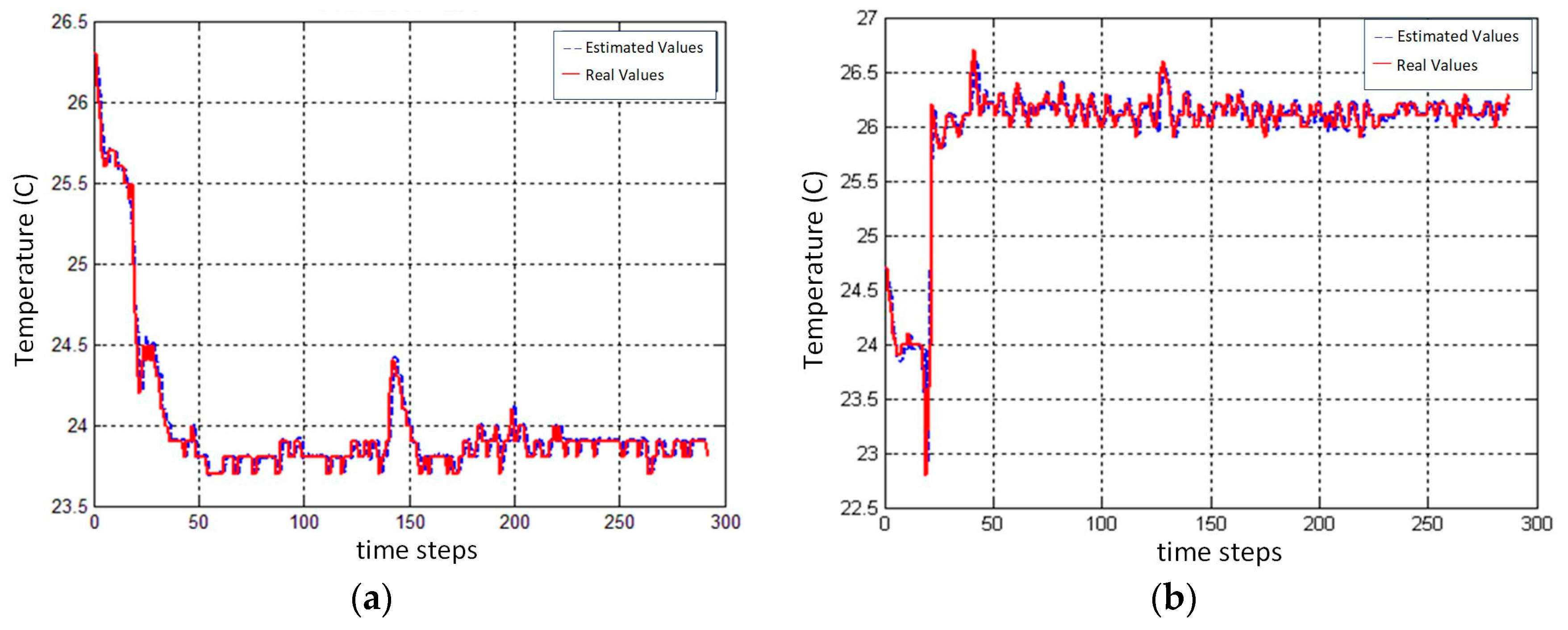
In order to verify the modeling capability of the proposed three FNN models in Equations (14)–(16), 52 weeks (or 12 months) of data between inputs and output for these three models are recorded for training and testing. One day among 7 days in a week is randomly selected for testing. In other words, the data contained in 6 days a week, 52 weeks a year, are utilized for training. The rest of 52 weeks of data, i.e., one randomly selected day a week, 52 weeks a year, are utilized for testing. The RMSE defined in (17) for the training and testing results are shown in

Table 1. Comparison of RMSE of estimated signals for training and testing results.

Estimated Signals	FNN Structure	Facilities	RMSE (Training)	RMSE (Testing)	RMSE (A Typical Testing Day)
$P_{ch}$ (power consumption of chiller)	1 × 10 × 10 × 1	Chiller 1	1.1246	1.1367	1.1129 (Figure 3a)
		Chiller 2	0.9829	0.8825	0.6838 (Figure 3b)
$P_{AHU}$ (power consumption of AHU)	1 × 10 × 1	AHU 1	0.0241	0.0257	0.0311 (Figure 4a)
		AHU 2	0.0267	0.0299	0.0215 (Figure 4b)
$T_f$ (AHU outlet cold air temperature)	5 × 15 × 15 × 1	AHU 1	0.1125	0.1324	0.1227 (Figure 5a)
		AHU 2	0.1087	0.1138	0.1018 (Figure 5b)

. It is shown in Table 1 that the RMSE for testing data are not too different from the one for training. The modeling accuracies of the proposed three FNN models are thus guaranteed. For the purpose of illustration, the power consumptions of chiller and AHU as well as the AHU outlet cold air temperature estimated by those three FNN models for a typical testing day are compared with real data in Figure 3a,b, Figure 4a,b and Figure 5a,b, respectively. From the RMSE of the data on this typical testing day in Table 1 and the modeling results illustrated in Figure 3, Figure 4 and Figure 5, the modeling accuracy of these three FNN models can also be verified.

5.2. Experiments of Energy Saving

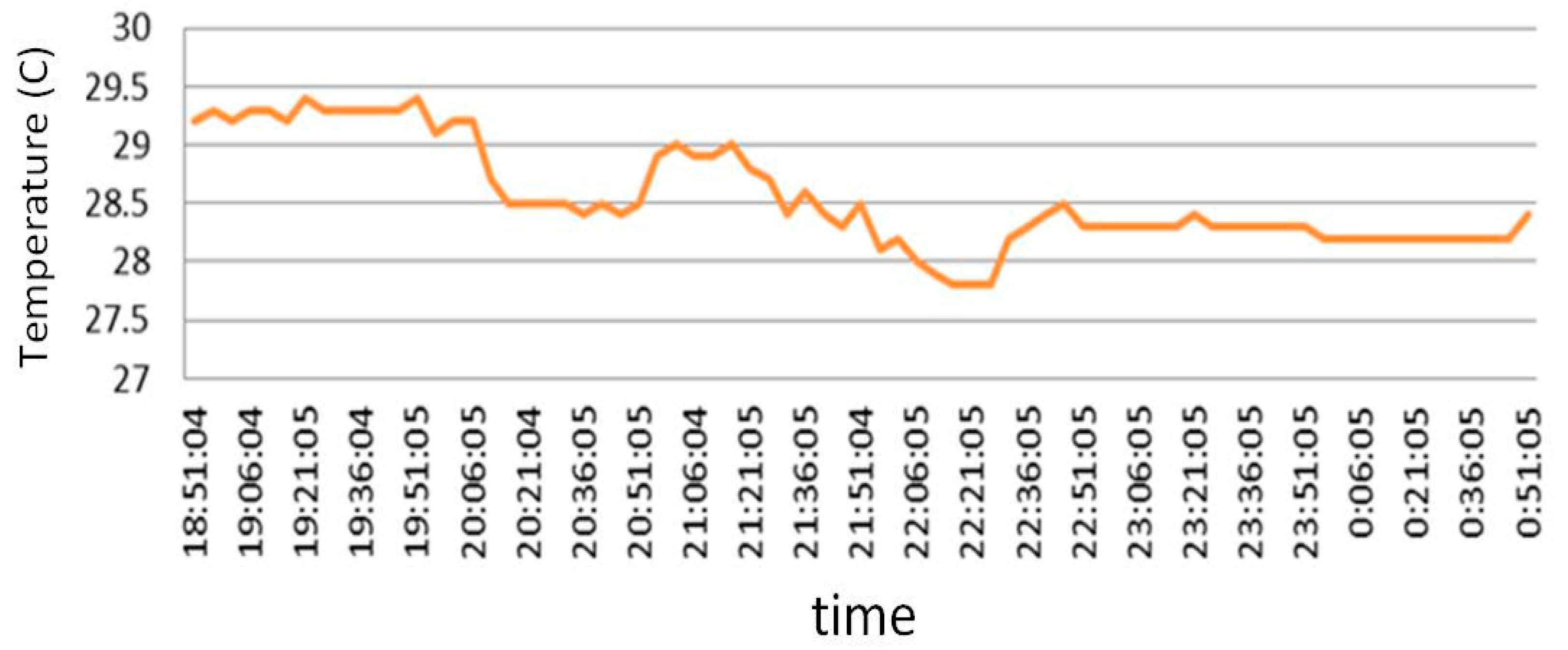
In order to signify the effectiveness and efficiency of the proposed energy saving control scheme, the control scheme was applied from 19:50 to 23:50 on a typical summer night. It takes about 120 s in every sampling interval for the energy saving controller running the proposed multi-objective optimization and returns both optimization variables $T_{chwo}$ and $v_f$ at every time step on a personal computer with Intel^® Core™ i7-8700 CPU @ 3.20 GHz. The variation in outdoor temperature is shown in Figure 6. For the convenience of illustration, vertical black bars are added in Figure 7, Figure 8, Figure 9 and Figure 10, showing the start and end of the control interval. It is shown in Figure 7 that the AHU outlet cold air temperature $T_f$ started dropping a few minutes after the control scheme was applied at 19:50 and went up a few minutes after the control scheme was terminated. Figure 8 shows that the variations in $T_{chwo}$ calculated by the proposed multi-objective optimization approach and the ones practically measured in the field. It is shown in Figure 8 that the measured values did follow the calculated ones.

In response to the calculated and measured chilled water outlet temperature, the chiller power consumption went down as the control interval started and returned to normal values as the control interval ended, showing the energy saving performance of the proposed control scheme. Since the running speed $v_f$ of the AHU fans was adjusted using a pulse width modulation (PWM) controller, the variation in calculated $v_f$ was in duty cycles as shown in Figure 9. Referring to Figure 9, the AHU power consumption within the control interval slightly increases. It leads to AHU outlet cold air temperature $T_f$ going down within the control interval as shown in Figure 7. Although AHU power consumption slightly increased, chiller power consumption went down during the control interval. The total power consumption of both chiller and AHU is shown in Figure 10. Figure 10 shows that the total power did reduce within the control interval. The PUE before the control interval is 1.55 and yet the PUE within the control interval drops to 1.42. The RCI_LO and RCI_HI before the control interval was applied were 100% and 93%, respectively, while both values are 100% within the control interval.

The same experiment was also conducted on a whole day in both summer and winter, calculating average energy saving. The energy saving effect was verified by comparing a pair of days with and without the proposed energy saving control scheme. These two days were selected for experiments under the condition that they had similar average outdoor temperatures and similar average CPU loads for the IOT equipment. The evaluation interval ranges from 9:00 a.m. to 5:00 p.m. within a regular campus working interval. The energy saving performance on a typical winter day and summer day with and without the proposed energy saving control scheme is shown in

Table 2. Comparison of energy saving performance with and without control.

Season	Control Status	Avg. Outdoor Temp. (°C)	Avg. Power Consumption (kW)	Avg. Energy Saved (kWh/h)	Avg. PUE	Avg. Outlet Cold Air temp. Tf (°C)
Winter day	W/control	19.95	11.74	4.02	1.4	24.33
	W/o control	17.2	15.76	-	1.52	24.58
Summer day	W/control	25.66	12.52	3.05	1.42	24.11
	W/o control	26.33	15.57	-	1.53	24.27

. Table 2 shows that the average energy saved on a typical winter day and summer day is 4.02 kWh/h and 3.05 kWh/h, respectively. The energy saving ratios are 23.4% and 19.6% for a typical winter and summer day, respectively. Table 2 also shows that the average outlet cold air temperature $T_f$ is not affected by the energy saving control despite the fact that significant energy saving results has been achieved. In fact, it is even slightly reduced on the day with energy saving control. It shows that the proposed energy saving control scheme can save the consumed energy and also maintain the rack inlet air temperature within a suitable range satisfying RCI.

6. Conclusions

A multi-objective optimization approach NSGA-II was proposed to optimize energy saving effectiveness. The optimization approach minimizes the power consumptions of both chillers and AHUs while keeping AHU outlet cold air temperature within a specified range. Both commonly used standardized metrics for data centers including PUE and RCI were utilized as the objects for optimization. Fresh air cooling control can also be integrated with the proposed energy saving control scheme to further improve energy saving performance. In fact, the proposed energy saving control scheme can also be applied to other central ACS controlling both chillers and AHUs. Neural network models are utilized to model the power consumption of chillers and AHUs, as well as the prediction of AHU outlet cold air temperature. Other models such as recurrent neural network (RNN) and long short-term memory (LSTM) can also be used if the data center size is too large or the airflow loop distance is too long.

References

- Shehabi, E.M.; Price, H.; Horvath, A.; Nazaroff, W.W. Data center design and location: Consequences for electricity use and greenhouse-gas emission. Build. Environ. 2011, 46, 990–998. [Google Scholar] [CrossRef]
- Cho, J.; Kim, B.S. Evaluation of air management systems’ thermal performance for superior cooling efficiency in high density data centers. Energy Build. 2011, 43, 2145–2155. [Google Scholar] [CrossRef]
- Khalaj, A.H.; Scherer, T.; Halgamuge, S.K. Energy environmental and economical saving potential of data centers with various economizers across Australia. Appl. Energy 2016, 183, 1528–1549. [Google Scholar] [CrossRef]
- Ni, J.; Bai, X. A review of air conditioning energy performance in data centers. Renew. Sustain. Energy Rev. 2017, 67, 625–640. [Google Scholar] [CrossRef]
- Beaty, D.L. Internal IT load profile variability. ASHRAE J. 2013, 55, 72–74. [Google Scholar]
- Shehabi, A.; Smith, S.J.; Sartor, D.A.; Brown, R.E.; Herrlin, M.; Koomey, J.G.; Masanet, E.R.; Horner, N.; Azevedo, I.L.; Lintner, W. United States Data Center Energy Usage Report. 2016. Available online: https://eta.lbl.gov/publications/united-states-data-center-energy (accessed on 1 March 2018).[Green Version]
- ASHRAE. ASHRAE Guidelines for Data Processing Environments. 2011. Available online: https://ecoinfo.cnrs.fr/IMG/pdf/ashrae_2011_thermal_guidelines_data_center.pdf (accessed on 1 March 2018).
- Avelar, V.; Azevedo, D.; French, A. PUE: A Comprehensive Examination of the Metric; White Paper #49; The Green Grid. 2012. Available online: https://www.thegreengrid.org/en/resources/library-and-tools/237-PUE%3A-A-Comprehensive-Examination-of-the-Metric (accessed on 1 March 2018).
- Yuventi, J.; Mehdizadeh, R. A critical analysis of power usage effectiveness and its use in communicating data center energy consumption. Energy Build. 2013, 64, 90–94. [Google Scholar] [CrossRef]
- Brady, G.; Kapur, N.; Summers, J.; Thompson, H. A case study and critical assessment in calculating power usage effectiveness for a data center. Energy Convers. Manag. 2013, 76, 155–161. [Google Scholar] [CrossRef]
- Herrlin, M.K. Rack cooling effectiveness in data centers and telecom central offices: The rack cooling index (RCI). ASHRAE Trans. 2005, 111, 725–731. [Google Scholar]
- Norouzi-Khangah, B.; Mohammadsadeghi-Zzad, M.B.; Hoseyni, S.M.; Hoseyni, S.M. Performance assessment of cooling systems in data centers; Methodology and application of a new thermal metric. Case Stud. Therm. Eng. 2016, 8, 152–163. [Google Scholar] [CrossRef] [Green Version]
- Chu, W.-X.; Wang, C.-C. A review on airflow management in data centers. Appl. Energy 2019, 240, 84–119. [Google Scholar] [CrossRef]
- Karki, K.C.; Patankar, S.V. Airflow distribution through perforated tiles in raised-floor data center. Build. Environ. 2006, 41, 734–744. [Google Scholar] [CrossRef]
- Nada, S.A.; Said, M.A. Comprehensive study on the effects of plenum depths on air flow and thermal managements in data centers. Int. J. Therm. Sci. 2017, 122, 302–312. [Google Scholar] [CrossRef]
- Nagarathinam, S.; Fakhim, B.; Behnia, M.; Armfield, S. A comparison of parametric and multivariable optimization techniques in a raised floor data center. J. Electron. Packag. 2013, 135, 030905. [Google Scholar] [CrossRef]
- Patankur, S.V.; Karki, K.C. Distribution of cooling airflow in a raised floor data center. ASHRAE Trans. 2004, 110, 629–634. [Google Scholar]
- Sorel, V. The oft-forgotten component of air flow management in data center applications. ASHRAE Trans. 2011, 117, 427–432. [Google Scholar]
- Arghode, V.K.; Joshi, Y. Modeling strategies for air flow through perforated tiles in a data center. IEEE Trans. Compon. Pack. Manuf. Technol. 2013, 3, 800–810. [Google Scholar] [CrossRef]
- Arghode, V.K.; Joshi, Y. Experimental investigation of air flow through a perforated tile in a raised floor data center. J. Electron. Packag. 2015, 137, 011011. [Google Scholar] [CrossRef]
- Demetriou, D.W.; Khalifa, H.E. Optimization of enclosed aisle data centers using bypass recirculation. J. Electron. Packag. 2012, 134, 020904. [Google Scholar] [CrossRef]
- Erdent, H.S.; Koz, M.; Yildirim, M.T.; Khalifa, H.E. Experimental demonstration and flow network model verification of induced CRAH bypass for cooling optimization of enclosed-aisle data centers. IEEE Trans. Compon. Pack. Manuf. Technol. 2017, 7, 1795–1803. [Google Scholar] [CrossRef]
- Erdent, H.S.; Koz, M.; Yildirim, M.T.; Khalifa, H.E. Optimization of enclosed aisle data centers with induced CRAH bypass. IEEE Trans. Compon. Pack. Manuf. Technol. 2017, 7, 1981–1989. [Google Scholar] [CrossRef]
- Song, Z. Numerical cooling performance evaluation of fan-assisted perforations in a raised-floor data center. Int. J. Heat Mass Transf. 2016, 95, 833–842. [Google Scholar] [CrossRef]
- Song, Z. Thermal performance of a contained data center with fan-assisted perforations. Appl. Therm. Eng. 2016, 102, 1175–1184. [Google Scholar] [CrossRef]
- Arghode, V.K.; Sundaralingam, V.; Joshi, Y. Airflow management in a contained cold aisle using active fan tiles for energy efficient data-center operation. Heat Transf. Eng. 2016, 37, 246–256. [Google Scholar] [CrossRef]
- Gao, T.; Sammakia, B.G.; Geer, J.F.; Ortega, A.; Schmidt, R. Dynamic analysis of cross flow heat exchangers in data centers using transient effectiveness method. IEEE Trans. Compon. Pack. Manuf. Technol. 2014, 4, 1925–1935. [Google Scholar] [CrossRef]
- Sahini, M.; Kumar, E.; Gao, T.; Ingalz, C.; Heydari, A.; Sun, X.G. Study of air flow energy within data center room and sizing of hot aisle containment for an active vs. passive cooling design. In Proceedings of the IEEE Intersociety Conference Thermal and Thermomechanical Phenomena in Electronic System, Las Vegas, NV, USA, 31 May–3 June 2016; pp. 1453–1457. [Google Scholar]
- Wilson, M.; Wattelet, J.P.; Wert, K.W. A thermal bus system for cooling electronic component in high density cabinets. ASHRAE Trans. 2004, 110, 567–573. [Google Scholar]
- Liu, Y.; Yang, X.; Li, J.; Zhao, X. Energy savings of hybrid dew-point evaporative cooler and micro-channel separated heat pipe cooling systems for computer data centers. Energy 2018, 163, 629–640. [Google Scholar] [CrossRef]
- Taras, M.F. Is economizer cycle justified for AC applications. ASHRAE J. 2005, 47, 38–45. [Google Scholar]
- Jinkyun, C.; Taesub, L.; Kim, B.S. Viability of datacenter cooling systems for energy efficiency in temperate or subtropical regions: Case study. Energy Build. 2012, 55, 189–197. [Google Scholar]
- Biswas, S.; Tiwari, M.; Sherwood, T.; Theogarajan, L.; Ching, F. Fighting fire with fire: Modelling the datacenter-scale effect of targeted super lattice thermal management. In Proceedings of the ISCA 2011 38th International Symposium on Computer Architecture, San Jose, CA, USA, 4–8 June 2011. [Google Scholar]
- Durand-Estebea, B.; le Bot, C.; Mancos, J.N.; Arquis, E. Data center optimization using PID regulation in CFD simulations. Energy Build. 2013, 66, 154–164. [Google Scholar] [CrossRef]
- Durand-Estebea, B.; le Bot, C.; Mancos, J.N.; Arquis, E. Simulation of a temperature adaptive control strategy for an IWSE economizer in a data center. Appl. Energy 2014, 134, 45–56. [Google Scholar] [CrossRef]
- Wang, N.; Zhang, J.; Xia, X. Energy consumption of air conditioners at different temperature set points. Energy Build. 2013, 65, 412–413. [Google Scholar] [CrossRef]
- Zhuang, C.; Wang, S.; Shan, K. Adaptive full-range decoupled ventilation strategy and air conditioning systems for cleanrooms and buildings requiring strict humidity control and their performance evaluation. Energy 2019, 168, 883–896. [Google Scholar] [CrossRef]
- Qi, Q.; Deng, S.M. Multivariable control of indoor air temperature and humidity in a direct expansion (DX) air conditioning (A/C) system. Build. Environ. 2009, 44, 1659–1667. [Google Scholar] [CrossRef]
- Khan, M.W.; Choudhry, M.A.; Zeeshan, M.; Ali, A. Adaptive fuzzy multivariable controller design based on genetic algorithm for an air handling unit. Energy 2015, 81, 477–488. [Google Scholar] [CrossRef]
- Gaoa, J.; Xua, X.; Li, X.; Zhang, J.; Zhang, Y.; Wei, G. Model-based space temperature cascade control for constant air volume air conditioning system. Build. Environ. 2018, 145, 308–318. [Google Scholar] [CrossRef]
- Chuang, H.-C.; Zeng, Y.-X.; Lee, C.-T. Study on a chiller of air conditioning system by sensing refrigerant pressure feedback control with step less variable speed driving technology. Build. Environ. 2019, 149, 157–168. [Google Scholar] [CrossRef]
- Liao, Y.; Huang, G.; Ding, Y.; Wu, H.; Feng, Z. Robustness enhancement for chiller sequencing control under uncertainty. Appl. Therm. Eng. 2018, 141, 811–818. [Google Scholar] [CrossRef]
- Liu, Z.; Tan, H.; Luo, D.; Yu, G.; Li, J.; Li, Z. Optimal chiller sequencing control in an office building considering the variation of chiller maximum cooling capacity. Energy Build. 2017, 140, 430–442. [Google Scholar] [CrossRef]
- Chang, W.H.; Chen, C.; Lee, Y.; Huang, C.N. Simulated annealing based optimal chiller loading for saving energy. Energy Convers. Manag. 2006, 47, 2044–2058. [Google Scholar] [CrossRef]
- Wei, X.; Kusiak, A.; Li, M.; Tang, F.; Zeng, Y. Multi-objective optimization of the HVAC (heating, ventilation, and air conditioning) system performance. Energy 2015, 83, 294–306. [Google Scholar] [CrossRef]
- Kusiak, G.X.; Tang, F. Optimization of an HVAC system with a strength multi-objective particle-swarm algorithm. Energy 2011, 36, 5935–5943. [Google Scholar] [CrossRef]
- Magnier, L.; Haghighat, F. Multiobjective optimization of building design using TRNSYS simulations, genetic algorithm, and Artificial Neural Network. Build. Environ. 2010, 45, 739–746. [Google Scholar] [CrossRef]
- Kusiak, F.T.; Xu, G. Multi-objective optimization of HVAC system with an evolutionary computation algorithm. Energy 2011, 36, 2440–2449. [Google Scholar] [CrossRef]
- Deb, K.; Pratap, A.; Agarwal, S.; Meyarivan, T. A fast and elitist multiobjective genetic algorithm: NSGA-II. IEEE Trans. Evolut. Comput. 2002, 6, 182–197. [Google Scholar] [CrossRef] [Green Version]
Figure 1.
System structure of energy saving control for data center air conditioning system.
Figure 2.
Illustration of fitness value calculation for the chromosome in the gene pool.
Figure 3.
Comparison of chiller power consumptions between estimated and real values for (a) chiller 1; (b) chiller 2.
Figure 4.
Comparison of air handling unit (AHU) power consumptions between estimated and real values for (a) AHU 1; (b) AHU 2.
Figure 5.
Comparison of predicted and real AHU outlet cold air temperature for (a) AHU 1; (b) AHU 2.
Figure 6.
Outdoor temperature.
Figure 7.
AHU outlet cold air temperature.
Figure 8.
Calculated and measured chilled water outlet temperature and chiller power consumption.
Figure 9.
Running speed of AHU fans and AHU power consumption.
Figure 10.
Total power consumption of chiller and AHU.