Sustainable Zoning, Land-Use Allocation and Facility Location Optimisation in Smart Cities


1
Faculty of Built Environment, UNSW Sydney, Sydney 2052, Australia
2
School of Civil Engineering, The University of Sydney, Sydney 2006, Australia
3
Departamento de Construção Civil, Escola Politécnica da Universidade Federal do Rio de Janeiro, Athos da Silveira Ramos 149, Ilha do Fundão, RJ, Brazil
*
Author to whom correspondence should be addressed.
Energies 2019, 12(7), 1318; https://doi.org/10.3390/en12071318
Submission received: 2 January 2019
/
Revised: 11 March 2019
/
Accepted: 15 March 2019
/
Published: 5 April 2019
(This article belongs to the Special Issue Selected Papers from SDEWES 2018 Conferences on Sustainable Development of Energy, Water and Environment Systems)
Abstract
:Many cities around the world are facing immense pressure due to the expediting growth rates in urban population levels. The notion of ‘smart cities’ has been proposed as a solution to enhance the sustainability of cities through effective urban management of governance, energy and transportation. The research presented herein examines the applicability of a mathematical framework to enhance the sustainability of decisions involved in zoning, land-use allocation and facility location within smart cities. In particular, a mathematical optimisation framework is proposed, which links through with other platforms in city settings, for optimising the zoning, land-use allocation, location of new buildings and the investment decisions made regarding infrastructure works in smart cities. Multiple objective functions are formulated to optimise social, economic and environmental considerations in the urban space. The impact on underlying traffic of location choices made for the newly introduced buildings is accounted for through optimised assignment of traffic to the underlying network. A case example on urban planning and infrastructure development within a smart city is used to demonstrate the applicability of the proposed method.
1. Introduction
Existing statistics state that almost 55% of the population of the world currently resides in urban regions [1,2], with estimates that this rate will increase to 70% by 2050 [3]. As this progression towards greater urban centres continues to increase, a need has emerged to find ways for supporting this growth in a sustainable manner. Furthermore, there is the challenge of dealing with the pollution levels that result from exacerbated activities in cities [4]. Along with the surging rates of urbanisation and pollution, the world has also experienced a breakthrough in the use of technologies, specifically those related to information and communication technologies (ICT) [5]. Updates in connectivity between various electronic platforms has led to the development of the Internet of Things (IoT), which is based on networks formed between physical devices and appliances to allow data transfer and exchange for enhanced operations [6].
The integration of ICT and IoT is thought to lead to an enhanced system for the management of cities. As a result, the notion of smart cities has arisen in response to the need for sustainable cities that can accommodate the growing population numbers, hence enhancing cities’ liveability and the wellness and living standards of citizens [7]. Even though universal agreement on a specific definition of a ‘smart city’ is still lacking, its main domain lies in the use of information and ICT in sectors such as infrastructure, buildings and energy [8]. In particular, concepts from ICT and IoT are being increasingly reflected in the operations of existing cities, resulting in an interrelated platform between large numbers of citizens, transport networks, services and urban assets and facilities [9].
Decision-making in planning and operations of smart cities needs to be structured around two main considerations, namely strategic and tactical decisions [10]. Yet, current emphasis in the literature is on the technical interfaces making up the various data-exchange enabling platforms placed within the cities, with little emphasis on the strategic and tactical urban planning aspects of smart cities. Within the area of strategic decision-making in city planning, zoning of the city and the location of its operating facilities, including schools, hospitals and so forth, are both of significant relevance [11]. An appropriate selection of zone clusters and the subsequent selection of locations to place buildings in form the main components that are involved in city design. In cities, the positioning of new buildings leads to the generation of traffic demand in the existing network structure [12]. This causes additional traffic loadings on the existing network, and if not well planned for, can result in major transportation delays to network users. Traffic congestion is thought to result in over $121 billion in losses [13] and can increase the amount of carbon emissions from traffic by more than 53% [14]. Another important strategic consideration is the development of the underlying travel network of the region. Specifically, the development of the transport network will be based on the capacities required to handle the initiated travel on the transport networks, while the operations of the network will in turn be associated with the established capacity of the network, along with the traffic loading patterns on the links (roads) of the network. Decisions related to the transport network are determined based on population rates and estimated travel via the various transport modes utilised in the region [15]. As a result, the zoning of the city will have a direct impact on the locations available for the facilities required to service the underlying population, which in turn would also impact the traffic and operation of the transportation network [16]. It is vital to thus integrate the decision-making that is involved in the zoning, facility location and transport network capacity design of the underlying smart city.
The attention in this article is directed towards the concept of location planning in smart cities. The proposed approach can be divided into three main areas: (i) the need for establishing a framework for the construction of a smart city from scratch, where zoning and land use need to be specified; (ii) the location of buildings in smart cities and the investment decisions made regarding the expansion of the existing road network structure and capacity, which involves the consideration of attributes that influence the decision of positioning buildings such as schools, hospitals and offices; and (iii) the determination of the resulting impacts caused by such location decisions based on the triple bottom-line of sustainability, via formulation of appropriate social, environmental and economic cost objective functions. As a result, three main decisions, which form the essence of urban planning and design in smart cities are targeted: namely, the decisions made regarding the allocation of zones and the assignment of buildings to locations in the region, the expansion decisions related to the road structure of the city and the expansion of the capacity of existing links in the network (if one already exists).
In this paper, a range of mathematical optimisation problems are integrated, including the clustering problem [17], the assignment problem [18], the facility location problem [19] and the urban traffic design problem [12], in order to model key strategic decisions in smart city design and planning. The work proposed herein is expected to form an integral component of the urban design of smart cities. In particular, such a framework will find applicability in prospective smart city planning designs, to ensure a sustainable and integrated city structure where buildings and road networks are strategically planned for. The framework can be used both for new smart city development and for decisions to be made within an existing smart city and which impact the urban design morphology of the existing city.
Remainder of this article is divided as follows: the next section provides a review of the literature on smart city planning in terms of zoning, facility location and transport network design. The proposed mathematical optimisation framework for strategic planning of smart cities is then presented. Following that, the algorithm and formulations developed are outlined. A numerical example of a case project is used to validate the proposed framework. Concluding remarks are provided at the end.
2. Literature Review
A significant number of research studies examine the concept of smart city and its use for sustainable urban planning. The literature reviewed herein falls under, but is not limited to, one of the following fields that are imperative building blocks in smart cities: energy management, city structure zoning and location, intelligent transport systems and smart infrastructure.
Key aspects regarding IoT and its use in smart cities were reviewed in [20]. A bibliometric analysis in [21] examines frequent city categorisation, including smart cities, used for sustainable urbanisation. A comprehensive review was conducted in [22] for energy management and sustainable planning in smart cities [23]. Spatiotemporal forecasting methods, which exploit time series data from various locations within the context of smart cities, and their applications for smart city transport and building management were evaluated in [24].
Several studies focused on energy management in smart cities [25]. Wojnicki and Kotulski [26] proposed an outdoor lighting control system for smart cities. An activity-aware system to automate building systems in smart cities was developed in [27]. A framework to optimise energy management on smart campuses was proposed in [28]. A heating and cooling modelling system was proposed for minimising electricity consumption in smart cities [29]. A smart city architecture was developed in [30] for addressing challenges in smart grid distribution. A comparative assessment of smart energy systems to ensure sustainable, clean and reliable energy in smart cities is found in [31].
In terms of location optimisation, the authors of [32] proposed an optimisation approach that relies on integrating geographic information systems (GIS) with a fuzzy-analytical hierarchy process (FAHP) for choosing suitable wind farm sites. Impacts of location choices made on wind turbine operations were discussed in [33]. In the context of infrastructure planning for smart cities, the authors of [34] developed a city navigation approach for electric vehicles, where locations of charging stations were assumed to be unknown. A business model tool for smart cities to facilitate undertaking strategic decision-making promptly was proposed in [35]. In [36], a localisation-based key management system for meter data encryption in smart cities was proposed. The utilisation of smart parking lots in smart cities was investigated in [37].
In terms of urban planning and structuring, an integrated model which considers land use, transportation and energy systems for future smart cities was presented in [38]. A framework for a smart city in China, which focuses on use of big data for infrastructure city planning and management, was developed by the authors of [39]. Use of smart technology for enhancing the sustainability of the construction sector through targeting demolition waste was discussed in [40]. Even though an investigation on algorithms deployed for sustainable transport policy in cities has been carried out, as detailed in [41], there is no link that has been developed to account for location decisions of new buildings and their impacts on the smart city urban design structure. New ways to achieve systematic-based solutions that augment the process adopted in urban design and planning, and which can lead to future viability and prosperity in metropolitan regions, need to be developed.
As is apparent, there is little focus on developing mathematical optimisation models that integrate location and transportation decisions for use in urban design of smart cities. In particular, there is an apparent lack in studies that focus on addressing operational research problems that are relevant to the strategic planning of urban areas. This is especially imperative in urban design of smart cities, where emphasis on the interconnectivity of key features within the city environment, including transportation systems and adjoining city layout, is highly regarded. As a result, in this work, the aspect within smart city design which will be examined refers to an automated and systematic urban planning procedure that relies on the use of mathematical optimisation frameworks. Such mathematical frameworks can be utilised for a range of applications in smart cities, including intelligent transport planning systems, intelligent energy monitoring and delivery and smart urban design approaches. The main contributions of this study are as follows: (i) the development of a mathematical method for dividing the proposed smart city region into zonal clusters; (ii) formulation of an assignment problem for land-use selection in zonal clusters; and (iii) development of a mathematical framework for enhancing the sustainable planning of location decisions made regarding building placement, and for measuring their impact on the routing of traffic within the smart city, through automated infrastructure investment decisions. The research presented herein thus integrates strategic aspects of location planning and traffic assignment involved in the urban design of smart cities. The next section outlines the main components making up the developed framework.
3. Smart City Zoning, Facility Location and Transport Network Planning Framework
The main motivation behind the framework proposed in this study is to ensure the efficient planning and design of city zoning, building location and transport network of smart cities, while accounting for environmental, social and economic considerations. As was previously discussed, the layout and location planning decision in smart cities considers two main planning aspects, namely strategic and operational planning; this is displayed in Figure 1. As can be seen, in terms of the strategic planning decisions, the main variables that need to be modelled in the proposed framework are the zoning of the region, the link expansion variables on the existing network, network extension through addition of new links, and the positioning of buildings. Apart from future population growth, which creates a slight increase in the demand induced in the regions, the focus in the developed framework is mostly on traffic demand generated by the placement of buildings.
An outline of the proposed framework in this paper is shown in Figure 2. Three main decisions, which form the essence of urban planning and design in smart cities are targeted: namely, the decisions made regarding allocation of zones and the assignment of buildings to locations in the region, the expansion decisions related to the road structure of the city and the expansion of the capacity of existing links in the network (if one already exists). The main concept introduced via the developed framework is the vital integration of all three decisions into a single model that simultaneously optimises the decision-making process involved.
The strategic decision for smart cities starts with the division of the region into zones, assuming the subject is a new city that requires zoning. This step also involves determining the land-use patterns in the region. In the case that an already existing smart city is considered, then the zoning procedure can be neglected, and the existing zonal configuration can be adopted instead. The second step involves the positioning of the buildings within the zones defined and in accordance with the allocated land-use patterns. Examples of buildings that need to be located include offices, retail shops, hospitals and schools. The third step is that related to infrastructure development and expansion. Such decisions will be influenced by the previous two steps and so it is necessary to assimilate both decisions together in a fashion that permits the translations of the impacts that the zoning and location decisions have on the infrastructure investment decisions made by the planners.
Given that a chief consideration in smart cities is ensuring effective mobility and robust decision-making for improving the transport of goods and people, developing an approach that can incorporate a forward-looking method for assignment of traffic based on newly introduced buildings is thus imperative. To enable this to happen, a multi-objective optimisation model is developed, based on a bilevel structure [42]. The bilevel structure is needed in order to model the decision spaces of the two main decision-makers in the model: namely, the urban planners and the transportation network users. The importance of generating sustainable solutions that target the triple bottom-line of sustainability is also accounted for through considering objective functions in the optimisation model developed, with focus on environmental, social and economic impacts of the locations and infrastructure decisions made.
The model can then be adapted to continue to be utilised for the strategic decisions to be made within the smart city, whenever a change in the structure of the city is induced. The change that is emphasised in the framework is related to the introduction of a new zone or building within the region. As shown in Figure 2, the procedure loops back to the optimisation model, whose associated parameters are updated in response to the induced changes, and a new solution is generated. Otherwise, if no change is induced, the algorithm ceases.
The proposed framework can also be linked to other automated systems that rely on the use of ICT in daily management of the city, such as online estimation of origin–destination (OD) matrices within the city for enhanced traffic assignment and real-time traffic state estimation and updates [43]. The work in this article is specifically targeted towards enhancing the intelligence of the transport systems through considering the impacts of newly positioned buildings on the underlying network.
4. Mathematical Optimisation Models
In this section, the mathematical formulations that are integrated in the proposed framework are outlined. The mathematical optimisation models can be divided into three main types: the first is associated with the zone division and clustering in the region, the second relates to the assignment of land-use patterns to the zone clusters and the third is related to the location of buildings and traffic assignment to the underlying network, based on infrastructure decisions made in the region. Notations adopted in the proposed mathematical models are given in Nomenclature.
4.1. Zoning Regions
Assuming an input of free land dispersed in the region is provided by the decision-maker (urban planner), the first step in zoning a smart city involves clustering the land into discrete zones. This step will involve the use of a clustering algorithm in order to yield a layout of area nodes clustered into zones. The second step involves assigning a land-use zone to each cluster created via the clustering algorithm. Each of these steps will now be explained.
4.1.1. Area Clustering
Each available area is clustered into a set of zones via the use of a clustering algorithm. In this study, principles from the k-means clustering approach are adopted [44]. The algorithm is summarised in Figure 3.
Let be the coordinate of the area nodes and let denote the centroid of the zones to be created in the region. The underlying urban space should already contain the available spaces for region development, referred to as the nodes (see Figure 3A). The algorithm starts by placing an input number of zone centroids in the urban space at random, as demonstrated in Figure 3B. The aim is to then group the nodes into clusters, forming the discrete zones of the region. The algorithm iterates through all nodes present in the region, finding the nearest centroid to each node, according to Equation (1).
where ) is a distance function.
Once all nodes have been iterated through, a centroid is allocated to one or more nodes, as demonstrated via the hatching displayed in Figure 3C. The algorithm then recalculates the position of each centroid based on the following equation, Equation (2):
where set is the set of all area nodes allocated to the centroid in the previous step.
Equation (2) considers the average sum of all area node coordinates clustered around a specific zone centroid as the determining attribute of the updated centroid position.
4.1.2. Assignment Model
Once the zone clusters are formed, the next step involves developing an assignment model that allocates each zone to a specific land use in accordance with a given set of criteria. As an example, the criteria can be based on distance to existing roads, soil surface type of each zone cluster, distance to cities/towns nearby, etc. In this study, the assignment model developed is represented via a binary integer programming formulation, where an objective function based on a defined set of criteria is utilised. One of the common criteria used in zoning is the travel distance between zones. As a result, the objective function in this study is formulated to minimise the travel between the different land-use patterns, based on predications of travel of people within the region. Let and denote the set of land-use and zonal clusters available, let denote the people that are expected to travel between land use and (e.g., between commercial and residential zones) and let denote the distance of travel between zone cluster and . The integer variable is defined to equal to 1 if land use is assigned to zone cluster , and 0 otherwise. The objective function to be minimised (total distance of travel between land uses allocated to zones), is given as Equation (3):
Essential constraints that are defined are assignment constraints, which specify that each land use that planners intend to position in a given region are assigned to a particular land zone, as given by Equation (4):
The domain of the binary variables is defined in Equation (5):
Additional sets of constraints that specify other requirements, such as distances that are required between land uses and required connections to existing roads, etc., can also be formulated. It is also important to note that other objective functions that target other criteria can be formulated for assignment of land-use areas to zonal clusters identified. The distance criterion was adopted in this study due to its high relevance in zone planning in urban regions.
4.2. Building Location and Infrastructure Model
Once the zonal configuration and land use specified for each zone is obtained, the next step involves formulating a model to (i) locate buildings in the region and (ii) determine the investment expansions required for existing infrastructure in response. A bilevel model [42] is proposed which accounts for the decision of two key decision-makers in a smart city setting, namely the urban planners and the transportation network users. The decision space of urban planners is modelled through optimising decisions related to the sustainability of the locations chosen for the buildings within the urban region, along with optimising the infrastructure investment decisions. The decision space of the network users is modelled through optimising their choice of links within the network in response to congestion created and demand generated when an urban planner places new buildings. Since the transport users respond to changes induced by decisions made by urban planners, the model proposed is developed based on a two-level hierarchical system, where the upper level represents the optimisation of the urban planners’ decision, while the lower level models the behaviour of users in response to decisions made by urban planners.
The upper level of the proposed model is described next.
4.2.1. Upper Level
The main decision variables in the upper level are: (i) the location decision, represented by the binary variable and which equals 1 if building is placed in location , and 0 otherwise; (ii) the binary variable , which specifies whether link ) is constructed or not; and (iii) the continuous variable , which indicates whether an existing link of the network is expanded or not.
Upper-Level Objective Functions
The upper-level model involves the formulation of three objective functions; each function targets one specific measure of sustainability. The first equation modelled is a proxy for the social pillar of sustainability (Equation (6)); it minimises the total noise pollution experienced in each zone of the smart city. Noise is generated by the buildings to be positioned in the region, as measured by the parameter .
Equation (7) targets the economic aspect of sustainability, where the cost of constructing buildings in the zones of the urban region, , is minimised.
The final objective function, Equation (8), considers the minimisation of the total carbon emissions from users on the traffic network. Equation (8) accounts for the emissions from different transportation modes, , which is multiplied by (i) the distance of the links of the network, ; (ii) the flow on the links, ; and (iii) the time of travel on the links of the network, which considers the congestion impacts on the roads, as given by Equations (9) and (10).
where denotes the free flow travel time, while and denote the existing capacity and the upgraded capacity of link , respectively.
In particular, Equations (9) and (10) represent the BPR link cost function developed by the Bureau of Public Roads (BPR) [45], which accounts for congestion. Equations (9) and (10) encompass the decisions related to the expansion of the network in order to determine the impacts on congestion levels in the network. Specifically, Equation (9) considers the link addition decisions, , while Equation (10) applies for all other link types that fall into , apart from the new links .
Upper-Level Constraints
A number of constraints are defined in the upper-level model to delineate part of the decision space of the urban planners. In particular, Equation (11) specifies that each building is to be positioned in a node within the region.
Equation (12) indicates that each node should host at most a single building:
Equation (13) is a budget constraint to ensure that investment decisions related to network expansion are kept under control.
The domain of the upper-level variables is defined by Equations (14)–(17).
4.2.2. Lower Level
People within the smart city will attempt to reduce their individual travel times when travelling on the transportation network. These decisions will highly depend on the changes induced by decisions made by urban planners, in terms of both the location of new buildings and network expansion decisions related to infrastructure investment.
Lower-Level Objective Functions
Since the transport network users will attempt to minimise their individual travel times, this sort of selfish behaviour of users can be modelled via a user equilibrium (UE) traffic assignment model [46], such as Equation (18).
Lower-Level Constraints
The lower-level constraints focus on the flow variable, to assign traffic to different links within the network. To ensure flow conservation at each node within the network, Equation (19) is defined.
In order to link the decision variable of the upper level with the decisions made by the lower level, Equations (20) and (21) are defined. In particular, Equation (20) states that flow from the location of the building to the sink node (which accumulates total travel on the network to the particular building type, i.e., single destination) is only possible if that specific building is located on the node from which the link emanates. Equation (21) states that total flow to all destinations on a proposed link within the network, , is not made possible unless the link is assigned to be constructed.
Equation (22) is a definitional constraint which specifies that the total flow on a given link is the sum of all flows heading towards all destinations, , on that respective link:
The domain of the lower-level decision variable is defined via Equation (23).
5. Solution Approach
The lower-level constraints focus on the flow variable in order to assign traffic to different links within the network. To ensure flow conservation at each node within the network, Equation (19) is defined.
In order to solve the proposed bilevel model above, a procedure which relies on converting the bilevel formulation into a single level model is adopted. A flow chart depicting the major steps undertaken is presented in Figure 4. In particular, the Karush–Kuhn–Tucker (KKT) equivalent conditions are used to reformulate the lower-level model, resulting in a single-level representation. The resulting single level is a mixed integer nonlinear programming (MINLP) model, which is then linearised through implementing a scheme that is based on piecewise approximation of the convex BPR function. Given that multiple objectives are considered at the upper level, a multi-objective optimisation solving approach is required. Lexicographic optimisation [47], which assumes a particular preference order over the criteria included, is adopted. The next section outlines the use of Karush-Kuhn-Tucker (KKT) conditions to reformulate the bilevel model.
5.1. Equivalent Lower-Level Model
The UE conditions of the lower-level program can be represented by a set of first-order equivalent constraints, namely the KKT conditions [42]. A dual variable is defined for Equation (19). Complementary slackness conditions of KKT, which are equivalent to the UE of the lower level and which require either or , are enforced by Equations (24) and (25).
Since Equation (25) involves the multiplication of two variables and is hence nonlinear, the single-level model cannot be solved using a linear solver. To overcome this, an appropriate linearisation scheme to reformulate Equation (25) needs to be applied, as demonstrated in the next section.
5.2. Linearisinng the KKT Conditions
Let be an auxiliary binary integer variable, which equals 1 if , and 0 otherwise. The complementary slackness condition, Equation (25), is replaced with the following set of constraints, Equations (26)–(28), resulting in the linearisation of KKT conditions:
where and are large positive constants.
5.3. Linearising the BPR Function
A chain of linked special ordered sets (SOS) conditions is implemented for linearising the BPR functions in Equations (9) and (10) [48]. The principle idea behind the SOS linearisation scheme adopted is shown in Figure 5. The domains of and (i.e., the two continuous variables in the BPR function) are partitioned into and regions, respectively, based on a grid point structure. With each grid point, a continuous variable, namely , is associated. A necessary condition is imposed on , which states that no more than four adjacent grid points can be nonzero. The flow and link capacity variables can then be represented by Equations (29) and (30), respectively:
where and are predefined, fixed values of flow and capacity, respectively, used in the piecewise linearisation of the BPR function.
The BPR function is then approximated by the linear formulation through Equations (31) and (32):
The conditions imposed on are given by Equations (33)–(36):
Equation (33) is the usual convex combination requirement in piecewise linear approximation. Two auxiliary continuous variables, and , are defined and these are embedded within Equations (34)–(36), so that at most, four adjacent variables of can be nonzero. The combination of Equations (34) and (36) specifies that two adjacent at most in the direction can be nonzero, while Equations (35) and (36) state that at most two adjacent at most in the can be nonzero. In particular, Equation (36) states that the variables, , are of a special ordered set (SOS) of Type 2 (i.e., SOS2), where a maximum of two of the latter variables that are adjacent can be nonzero. This becomes obvious from Figure 5, since for the grid structure shown and in accordance with the latter equations enforced, not more than two adjacent variables of and can be nonzero in the and directions, respectively. The SOS2 conditions are specified as follows in Equations (37)–(40):
The domain of the variables used to mimic SOS2 is given as follows by Equations (41)–(43):
5.4. Linearing Carbon Emissions Objection Function
To linearise the carbon emissions objective function, Equation (8) is replaced by the equivalent Equation (44):
where highlights the shortest travel time between origin and destination .
5.5. Lexicographic Optimisation
Given that the bilevel model proposed for the urban design of smart cities contains multiple objectives that need to be satisfied, no single solution will optimise all criteria at once. As a result, the concept of optimality adopted in single-objective optimisation is replaced with the concept of Pareto optimality.
A solution of a multi-objective optimisation problem is said to be Pareto optimal if there is no other feasible solution such that and for at least one index , , where is the set of objective functions solved in the multi-objective problem.
Lexicographic optimisation involves assigning a preference order over all objective functions considered and solving the problem over a number of stages [49]. In this paper, the lexicographic optimisation approach is adopted, given that it is likely that urban designers have a preference order defined over certain criteria when structuring a region. The algorithm developed is displayed in Algorithm 1.
| Algorithm 1 Lexicographic Optimisation |
 |
The notation adopted for the lexicographic optimisation process is given by the term , which indicates that the model is first solved by minimising the highest ranked objective,. Once an optimal solution is yielded, the model is re-solved by adopting as the objective function and by including the constraint in the model, where is the optimal solution of obtained at the initial stage. The final solution is that attained once all objective functions have been included as constraints, where is the set of all objective functions involved in the model.
6. Computational Results
In this section, the computational experiments utilised to demonstrate the applicability of the proposed optimisation framework are explained. In the first set of experiments, labelled Scenario 1, the framework is tested on a realistic example of a region being developed into a smart city. The structure of the city is displayed in Figure 6A. Figure 6B displays the available locations for positioning different buildings in the region. The type of buildings considered in the example include schools, hospitals, residential dwellings, offices, bus stops and factories. In the second set of experiments, multiple instances of network structures are generated in order to examine the performance of the proposed model. For both sets of experiments, the proposed mathematical optimisation models are coded in AMPL [50]; Python [51] is used as the programming language to generate instances in Scenario 2. The model is run on a personal computer with Intel Core i7, 2.2 GHz CPU and 8 GB RAM. CPLEX 12.7 is adopted as the linear solver [52].
6.1. Scenario 1
The first step of the framework involves partitioning the region into a number of zonal clusters. The k-means clustering algorithm of Figure 3 is utilised; the resulting zonal cluster is displayed in Figure 6A. A total of eight zonal clusters within the region have been identified. The next step involves assigning a land use to each zonal cluster. This enables the allocation of zones for positioning different building types in. This is achieved via the assignment model represented by Equations (3)–(5). It is desired to place four land-use zone types, namely three residential zones, two mixed-use zones, two commercial zones and one industrial zone. The resulting zones assigned are displayed in Figure 7B and Table 1. The building types desired to be placed, along with the associated maximum noise generated and noise sensitivity thresholds for each building, are displayed in Table 2.
The construction cost associated with each node is as follows: for nodes 1, 5, 7, 10, 17 and 18, construction cost is given as $503,124; for nodes 2, 3, 6, 13, 14, 15 and 19, construction cost is $209,353; and for nodes 4, 8, 9, 11, 12 and 16, the construction cost is given as $100,111.
The third stage involves an implementation of the strategic decision-support model for allocating buildings and determining the traffic assignment and any investments required in the connecting infrastructure of the region. Since the region is new, no existing network is present. A sample network shape utilised to outline the expected linking structure between the eight zones identified is depicted in Figure 8.
Lexicographic Optimisation Results
Let:
The preference assumed over the objective functions is given as follows: , where the relationship highlights the preferential ranking of in comparison to . In the first stage, the carbon emissions on the transport network, , are minimised (via minimising the total system travel time of the network). The emission factors associated with each transportation mode analysed in the smart city are given in Table 3, as obtained from [53]. Preference in the second stage is given to minimising the total sum of noise pollution within the region: . In the final stage of the lexicographic approach, the construction cost involved with constructing buildings at each location is minimised. Through applications of the lexicographic algorithm, the lexicographic Pareto optimal solutions obtained are displayed in Table 4. As is displayed, in the initial run, carbon emissions are minimised, while the rest of the objectives are evaluated (without being optimised yet). In the second lexicographic run, the carbon emissions remain at their minimum level, while noise pollution decreases by 45% and construction costs increase by 21%, in comparison to the first stage of the lexicographic run. In the third lexicographic run, both carbon emissions and noise pollution stay at their minimum levels (due to the constrained optimisation), while construction cost cannot be minimised further without violating the constraints placed on the carbon emissions and noise pollution functions.
6.2. Scenario 2
In the second set of experiments, the case example of Figure 5 is slightly modified to allow for an extensive computational analysis of the model developed. A total of 350 random instances are generated for examining the behaviour of the bilevel model. The size of the networks considered starts at 10 nodes and is incremented by 5 nodes until 40 nodes are reached. Travel distances are assumed to be proportional to the Euclidian distance between the zones, while buildings to be placed are assumed to be 40–90% of the number of nodes considered in the instance generated, in order to generate an encompassing set of scenarios. Figure 9 displays the average computational time required to yield an optimum solution, along with the percentage of instances solved to optimality within a 1000 s time limit. As can be seen, beyond 20 nodes, as the instance size increases, the average computation time increases and the percentage of instances solved to optimality decreases.
6.3. Comparison with Other Metaheuristics
In this section, common optimisation algorithm approaches adopted in the literature, including genetic algorithms (GA) [54] and particle swarm optimisation (PSO) [55], are contrasted with the proposed exact approach. Based on rigorous tests, the population size, mutation rate and crossover rate of 250, 0.05 and 0.7, respectively, were adopted in the GA, whereas for PSO, population size was set as 250, while acceleration constant and weight parameters were set as 3 and 0.4, respectively. As can be seen from Figure 10A, the solving time of the GA is better than both PSO and the proposed exact approach, though solution accuracy is better in the proposed exact approach. The results of Figure 10B highlight that even though the metaheuristic approaches can be faster in producing a solution, the solution quality of the exact approach will always be better. In addition, for the case considered herein, the fastest approach to generate a solution is obtained using a GA, though PSO can be slightly more accurate in terms of solution quality in contrast to the GA.
6.4. Multi-objective Variant
A pure Pareto-based formulation is applied, which relies on optimising all the objective functions simultaneously. The solution strategy adopted herein is referred to as the -constraint method, which relies on optimising a single objective function while accounting for the remaining objectives using constraints. A parametric variation of the right-hand side (RHS) of the constrained functions then ensues to generate the efficient Pareto points on the frontier. The reader is referred to [56] for additional information on the implementation of the -constraint method adopted.
The results obtained on application of the -constraint method to the case study presented above are displayed in Figure 11A–C. In addition, Table 5 presents the optimised values of extreme points used to plot the tradeoff curve. In Figure 11A, a clear tradeoff exists between minimising noise and minimising carbon-equivalent emissions. In Figure 11B, a tradeoff is shown between minimising layout cost and minimising noise, while Figure 11C displays the tradeoff between minimising layout cost and minimising carbon-equivalent emissions.
The importance of the Pareto curves produced lies in the fact that the decision-maker is now able to visualise the magnitude of the impact associated with each efficient solution produced.
6.5. Discussion and Insight
In comparison to some of the approaches in the literature, the proposed framework targets key strategic operational research problems that are encountered in the urban design of smart cities. For instance, in [57], the authors consider using integer optimisation to maximise floor area while accounting for sunlight in urban design. A mixed integer program was developed in [58] for designing building interiors. Integer programming was utilised in [59] for urban street network design. As can be noticed, there is a lack of focus on optimisation problems encountered in the strategic design of urban areas, where traffic and building layout are both integrated. The proposed approach in this article tackles this gap by proposing a mathematical optimisation model which integrates the latter. In addition, multiple objectives are rarely adopted in urban design optimisation [12]. As a result, through the proposed framework herein using multi-objective optimisation, the decision-maker can visualise the different tradeoffs that result when incorporating all objective functions considered.
7. Conclusions
Globally, we have witnessed a shift towards developing smart cities to deal with the challenges of rising population and urbanisation rates, along with the necessity of ensuring sustainable development. It seems therefore necessary to incorporate intelligent and robust urban planning frameworks that can simultaneously target transport and land-use considerations in smart cities.
In this paper, a framework, based on mathematical optimisation for the strategic planning of zoning, facility location and transport network design in smart cities was proposed. The framework combines some strategic operational research problems, including the clustering problem, the assignment problem, the facility location problem and the network design problem, in a systematic fashion. An algorithm based on k-means clustering is applied to divide a given region into zones, and an assignment problem is then solved to determine the land-use types within the region. The final stage of the framework involves solving a bilevel model that accounts for the hierarchical decision making of urban planners and travel network users. The proposed bilevel model considers the location decisions of buildings within a smart city setting, along with the investment decisions related to expansion of the underling transportation network. Multiple objective functions were formulated to target the triple bottom-line of sustainability in order to ensure a sustainable urban layout of the smart city. In particular, as a social factor, noise pollution in the region was minimised; as an environmental factor, carbon-equivalent emissions on the transportation network were minimised; and as an economic factor, the construction cost of buildings was minimised. A solution approach based on converting the bilevel model into a single-level model was outlined, along with a linearization procedure. A lexicographic optimisation approach was utilised to handle the multi-objective nature of the developed model. In addition, the -constraint method, which generates the Pareto front when considering all objective functions involved, was also adopted.
The proposed model was applied on a realistic case example for the design of the urban structure of a smart city. A lexicographic approach highlighted variations in cost of up to 52% when carbon emissions are given first preference by decision-makers. The-constraint method highlighted that a trade-off cost of up to 471% can result when simultaneously optimising the objective functions involved. In order to examine the computational performance of the proposed approach, a total of 350 instances were solved. Results demonstrate that solving time increased rapidly once the transportation network size of the instance generated exceeded 30 nodes. On average, the proposed model was able to solve 72% of the proposed instances within the imposed 1000 s time limit.
A comparison was also conducted between the proposed exact approach and metaheuristic solving algorithms including a GA and PSO. Results indicated that the GA was the fastest in terms of solution time, although solution accuracy was on average reduced by 68% compared to the results obtained when utilising the exact approach.
The proposed framework integrates several key operational research problems that are representative of certain aspects of the urban design problem involved in smart cities. However, several limitations are associated with the proposed approach. First, a deeper investigation into all facets of urban design that are associated with smart cities is lacking, since only several operational research problems are tackled in the framework developed. Second, the incorporation of tactic decision-making problems, such as vehicle routing, was missing from the proposed framework. Future works will thus look at these two areas.
Author Contributions
Conceptualization, A.WA.H. and E.G.V.; Data curation, A.WA.H.; Formal analysis, A.WA.H; Funding acquisition, E.G.V. and A.H.; Investigation, A.WA.H.; Methodology, A.WA.H, A.A., and A.H.; Supervision, E.G.V. and A.H.; Validation, A.H.; Writing—original draft, A.WA.H and A.A.
Funding
Authors would like to acknowledge the Brazilian Government for their support by the CNPq (National Council for Scientific and Technological Development)
Conflicts of Interest
The authors declare no conflict of interest.
Nomenclature
| Notation | Meaning |
| Type of building to be positioned in smart city | |
| Set of zone centroids to position in a region | |
| Set of land uses to define within the region | |
| Set of transport modes on the transport network | |
| Set of dummy nodes, acting as sink nodes for each building type | |
| Set of all building types | |
| Existing links that cannot be expanded | |
| Existing links that can be expanded | |
| New links that can be formed | |
| All link types that form the travel network | |
| Virtual links that connect to the sink node | |
| Set of potential locations for all building types | |
| Set of all nodes in the region | |
| Set of all destination nodes in the region | |
| Set of segments for linearising | |
| Set of segments for linearising | |
| Set of segments for linearising , less 1 | |
| Set of segments for linearising , less 1 | |
| Set of area node coordinates identified in the region, where | |
| Set of zonal coordinates of the region, where | |
| Set of all area nodes allocated to the centroid of a zone | |
| Set of all destinations | |
| Origin–destination (OD) matrix | |
| Cost of constructing a building at node | |
| Noise pollution assessed at node in the region, resulting due to a building placed at node | |
| Emission factors of transport mode in | |
| Distance between nodes | |
| Capacity of link | |
| Available budget for expansion of network | |
| A fixed parameter for the flow on link , used in the piecewise Linearisation of the BPR function | |
| A fixed parameter for the expanded capacity on link, used in the piecewise linearisation of the BPR function | |
| Large positive constants | |
| Binary variable, which equals 1 if land use is assigned to zone cluster , and 0 otherwise | |
| Binary variable, which equals 1 if type building, , is located at node , and 0 otherwise | |
| Binary variable, which equals 1 if link is added to the network, and zero otherwise | |
| Flow on link | |
| Amount of additional capacity added to link | |
| Auxiliary binary variable for linearising the KKT complementary slackness conditions | |
| Auxiliary binary variable for linearising the BPR function | |
| Auxiliary continuous variables for linearising the BPR function, for link and segment | |
| Continuous variable which highlights the shortest travel time between origin and destination | |
| Auxiliary continuous variables for linearising the BPR function | |
| Binary variable for mimicking SOS2 behaviour, defined over segments | |
| Binary variable for mimicking SOS2 behaviour, defined over segments | |
| Bureau of public roads (BPR); Karush-Kuhn-Tucker (KKT); Special Ordered Set 2 (SOS2) | |
References
- Li, B.; Yao, R. Urbanisation and its impact on building energy consumption and efficiency in China. Renew. Energy 2009, 34, 1994–1998. [Google Scholar] [CrossRef]
- United Nations. World Urbanisation Prospects: The 2018 Revision; UN DESA: New York city, NY, USA, 2018. [Google Scholar]
- UNICEF. Unicef Urban Population Map. 2017. Available online: https://www.unicef.org/sowc2012/urbanmap/# (accessed on 26 May 2018).
- Raimbault, M.; Dubois, D. Urban soundscapes: Experiences and knowledge. Cities 2005, 22, 339–350. [Google Scholar] [CrossRef]
- Vanolo, A. Is there anybody out there? The place and role of citizens in tomorrow’s smart cities. Futures 2016, 82, 26–36. [Google Scholar] [CrossRef]
- Slaughter, R.A. The IT revolution reassessed part three: Framing solutions. Futures 2018, 100, 1–19. [Google Scholar] [CrossRef]
- Ferraris, A.; Santoro, G.; Papa, A. The cities of the future: Hybrid alliances for open innovation projects. Futures 2018, 103, 51–60. [Google Scholar] [CrossRef]
- Kramers, A.; Höjer, M.; Lövehagen, N.; Wangel, J. Smart sustainable cities—Exploring ICT solutions for reduced energy use in cities. Environ. Model. Softw. 2014, 56, 52–62. [Google Scholar] [CrossRef]
- Park, E.; del Pobil, A.P.; Kwon, S.J. The Role of Internet of Things (IoT) in Smart Cities: Technology Roadmap-oriented Approaches. Sustainability 2018, 10, 1388. [Google Scholar] [CrossRef]
- Bekta, T.; Crainic, T.G.; van Woensel, T. From Managing Urban Freight to Smart City Logistics Networks. In Network Design and Optimization for Smart Cities; World Scientific: Quebec City, QC, Canada, 2016; Volume 8, pp. 143–188. [Google Scholar]
- Hammad, A.W.A.; Rey, D.; Akbarnezhad, A. A Bi-level Mixed Integer Programming Model to Solve the Multi-Servicing Facility. In Data and Decision Sciences in Action; Springer: Cham, Switzerland, 2018; pp. 381–395. [Google Scholar]
- Hammad, A.W.A.; Akbarnezhad, A.; Rey, D. Sustainable urban facility location: Minimising noise pollution and network congestion. Transp. Res. Part E Logist. Transp. Rev. 2017, 107, 38–59. [Google Scholar] [CrossRef]
- Djahel, S.; Jabeur, N.; Barrett, R.; Murphy, J. Toward V2I communication technology-based solution for reducing road traffic congestion in smart cities. In Proceedings of the 2015 International Symposium on Networks, Computers and Communications (ISNCC), Hammamet, Tunisia, 13–15 May 2015; pp. 1–6. [Google Scholar]
- Bharadwaj, S.; Ballare, S.; Rohit; Chandel, M.K. Impact of congestion on greenhouse gas emissions for road transport in Mumbai metropolitan region. Transp. Res. Procedia 2017, 25, 3538–3551. [Google Scholar] [CrossRef]
- Giles-Corti, B.; Vernez-Moudon, A.; Reis, R.; Turrell, G.; Dannenberg, A.L.; Badland, H.; Foster, S.; Lowe, M.; Sallis, J.F.; Stevenson, M.; et al. City planning and population health: A global challenge. Lancet 2016, 388, 2912–2924. [Google Scholar] [CrossRef]
- Cui, S.; Zhao, H.; Zhang, C. Locating Charging Stations of Various Sizes with Different Numbers of Chargers for Battery Electric Vehicles. Energies 2018, 11, 3056. [Google Scholar] [CrossRef]
- Brimberg, J.; Mladenović, N.; Todosijević, R.; Urošević, D. Local and Variable Neighborhood Searches for Solving the Capacitated Clustering Problem. In Optimization Methods and Applications; Springer: Cham, Switzerland, 2017; pp. 33–55. [Google Scholar]
- Patriksson, M. The Traffic Assignment Problem: Models and Methods; Courier Dover Publications: Utrecht, Netherlands, 2015. [Google Scholar]
- Karatas, M.; Yakıcı, E. An iterative solution approach to a multi-objective facility location problem. Appl. Soft Comput. 2018, 62, 272–287. [Google Scholar] [CrossRef]
- Talari, S.; Shafie-khah, M.; Siano, P.; Loia, V.; Tommasetti, A.; Catalão, J.P.S. A Review of Smart Cities Based on the Internet of Things Concept. Energies 2017, 10, 421. [Google Scholar] [CrossRef]
- De Jong, M.; Joss, S.; Schraven, D.; Zhan, C.; Weijnen, M. Sustainable–smart–resilient–low carbon–eco–knowledge cities; making sense of a multitude of concepts promoting sustainable urbanization. J. Clean. Prod. 2015, 109, 25–38. [Google Scholar] [CrossRef] [Green Version]
- Calvillo, C.F.; Sánchez-Miralles, A.; Villar, J. Energy management and planning in smart cities. Renew. Sustain. Energy Rev. 2016, 55, 273–287. [Google Scholar] [CrossRef]
- Deakin, M.; Reid, A. Smart cities: Under-gridding the sustainability of city-districts as energy efficient-low carbon zones. J. Clean. Prod. 2018, 173, 39–48. [Google Scholar] [CrossRef]
- Tascikaraoglu, A. Evaluation of spatio-temporal forecasting methods in various smart city applications. Renew. Sustain. Energy Rev. 2018, 82, 424–435. [Google Scholar] [CrossRef]
- Maier, S. Smart energy systems for smart city districts: Case study Reininghaus District. Energy Sustain. Soc. 2016, 6, 23. [Google Scholar] [CrossRef]
- Wojnicki, I.; Kotulski, L. Improving Control Efficiency of Dynamic Street Lighting by Utilizing the Dual Graph Grammar Concept. Energies 2018, 11, 402. [Google Scholar] [CrossRef]
- Thomas, B.L.; Cook, D.J. Activity-Aware Energy-Efficient Automation of Smart Buildings. Energies 2016, 9, 624. [Google Scholar] [CrossRef]
- Barbato, A.; Bolchini, C.; Geronazzo, A.; Quintarelli, E.; Palamarciuc, A.; Pitì, A.; Rottondi, C.; Verticale, G. Energy Optimization and Management of Demand Response Interactions in a Smart Campus. Energies 2016, 9, 398. [Google Scholar] [CrossRef]
- Sharma, S.; Dua, A.; Singh, M.; Kumar, N.; Prakash, S. Fuzzy rough set based energy management system for self-sustainable smart city. Renew. Sustain. Energy Rev. 2018, 82, 3633–3644. [Google Scholar] [CrossRef]
- Ruiz-Romero, S.; Colmenar-Santos, A.; Mur-Pérez, F.; López-Rey, Á. Integration of distributed generation in the power distribution network: The need for smart grid control systems, communication and equipment for a smart city—Use cases. Renew. Sustain. Energy Rev. 2014, 38, 223–234. [Google Scholar] [CrossRef]
- Dincer, I.; Acar, C. Smart energy systems for a sustainable future. Appl. Energy 2017, 194, 225–235. [Google Scholar] [CrossRef]
- Ali, S.; Lee, S.-M.; Jang, C.-M. Determination of the Most Optimal On-Shore Wind Farm Site Location Using a GIS-MCDM Methodology: Evaluating the Case of South Korea. Energies 2017, 10, 2072. [Google Scholar] [CrossRef]
- Ali, S.; Lee, S.-M.; Jang, C.-M. Techno-Economic Assessment of Wind Energy Potential at Three Locations in South Korea Using Long-Term Measured Wind Data. Energies 2017, 10, 1442. [Google Scholar] [CrossRef]
- García, R.M.; Prieto-Castrillo, F.; González, G.V.; Tejedor, J.P.; Corchado, J.M. Stochastic Navigation in Smart Cities. Energies 2017, 10, 929. [Google Scholar] [CrossRef]
- Díaz-Díaz, R.; Muñoz, L.; Pérez-González, D. The Business Model Evaluation Tool for Smart Cities: Application to SmartSantander Use Cases. Energies 2017, 10, 262. [Google Scholar] [CrossRef]
- Parvez, I.; Sarwat, A.I.; Wei, L.; Sundararajan, A. Securing Metering Infrastructure of Smart Grid: A Machine Learning and Localization Based Key Management Approach. Energies 2016, 9, 691. [Google Scholar] [CrossRef]
- Lanza, J.; Sánchez, L.; Gutiérrez, V.; Galache, J.A.; Santana, J.R.; Sotres, P.; Muñoz, L. Smart City Services over a Future Internet Platform Based on Internet of Things and Cloud: The Smart Parking Case. Energies 2016, 9, 719. [Google Scholar] [CrossRef]
- Yamagata, Y.; Seya, H. Simulating a future smart city: An integrated land use-energy model. Appl. Energy 2013, 112, 1466–1474. [Google Scholar] [CrossRef]
- Wu, Y.; Zhang, W.; Shen, J.; Mo, Z.; Peng, Y. Smart city with Chinese characteristics against the background of big data: Idea, action and risk. J. Clean. Prod. 2018, 173, 60–66. [Google Scholar] [CrossRef]
- Iacovidou, E.; Purnell, P.; Lim, M.K. The use of smart technologies in enabling construction components reuse: A viable method or a problem creating solution? J. Environ. Manag. 2018, 216, 214–223. [Google Scholar] [CrossRef] [PubMed]
- De Paula, L.B.; Marins, F.A.S. Algorithms applied in decision-making for sustainable transport. J. Clean. Prod. 2018, 176, 1133–1143. [Google Scholar] [CrossRef]
- Bard, J.F. Practical Bilevel Optimization: Algorithms and Applications; Springer Science & Business Media: Berlin, Germany, 2013. [Google Scholar]
- Nigro, M.; Cipriani, E.; del Giudice, A. Exploiting floating car data for time-dependent Origin–Destination matrices estimation. J. Intell. Transp. Syst. 2018, 22, 159–174. [Google Scholar] [CrossRef]
- Hartigan, J.A.; Wong, M.A. Algorithm AS 136: A k-means clustering algorithm. J. R. Stat. Soc. Ser. C Appl. Stat. 1979, 28, 100–108. [Google Scholar] [CrossRef]
- Transportation Research Board, National Research Council. Highway Capacity Manual; Transportation Research Board, National Research Council: Washington, DC, USA, 2000. [Google Scholar]
- Wardrop, J.G.; Whitehead, J.I. Some theoretical aspects of road traffic research. Proc. Inst. Civ. Eng. 1952, 1, 767–768. [Google Scholar] [CrossRef]
- Lam, T.B. Multi-Objective Optimization in Computational Intelligence: Theory and Practice: Theory and Practice; IGI Global: Pennsylvania, PA, USA, 2008. [Google Scholar]
- Beale, E.M.L. Integer Programming. In Computational Mathematical Programming; Schittkowski, K., Ed.; Springer: Berlin/Heidelberg, Germany, 1985; pp. 1–24. [Google Scholar]
- Ehrgott, M. Multicriteria Optimization; Springer Science & Business Media: Berlin, Germany, 2013. [Google Scholar]
- Fourer, R.; Gay, D.; Kernighan, B. Ampl: A Modeling Language for Mathematical Programming; DUXBURY, THOMSON Boyd & Fraser: Illinois, IL, USA, 1993; Volume 119. [Google Scholar]
- Van Rossum, T.G. Python tutorial, technical report. Technical report, Centrum voor Wiskunde en Informatica (CWI), Amsterdam, CS-r9526. May 1995. [Google Scholar]
- IBM, “CPLEX Optimizer,” 25 March 2019. Available online: https://www.ibm.com/analytics/cplex-optimizer (accessed on 5 January 2019).
- Spielmann, M.; Bauer, C.; Dones, R.; Tuchschmid, M. Transport Services. Swiss Centre for Life Cycle Inventories Dübendorf, Ecoinvent report 14. 2007. [Google Scholar]
- Konak, A.; Coit, D.W.; Smith, A.E. Multi-objective optimization using genetic algorithms: A tutorial. Reliab. Eng. Syst. Saf. 2006, 91, 992–1007. [Google Scholar] [CrossRef]
- Kennedy, J.; Eberhart, R.C. Particle swarm optimization. In Proceedings of the International Conference on Neural Networks, Perth, WA, Australia, 27 November–1 December 1995;–1948; Volume 1942–1948. [Google Scholar]
- Mavrotas, G. Effective implementation of the ε-constraint method in Multi-Objective Mathematical Programming problems. Appl. Math. Comput. 2009, 213, 455–465. [Google Scholar] [CrossRef]
- Hua, H.; Hovestadt, L.; Tang, P.; Li, B. Integer programming for urban design. Eur. J. Oper. Res. 2019, 274, 1125–1137. [Google Scholar] [CrossRef]
- Wu, W.; Fan, L.; Liu, L.; Wonka, P. MIQP-based Layout Design for Building Interiors. Comput. Graph. Forum 2018, 37, 511–521. [Google Scholar] [CrossRef]
- Peng, C.-H.; Yang, Y.-L.; Bao, F.; Fink, D.; Yan, D.-M.; Wonka, P.; Mitra, N.J. Computational network design from functional specifications. ACM Trans. Graph. TOG 2016, 35, 131. [Google Scholar] [CrossRef]
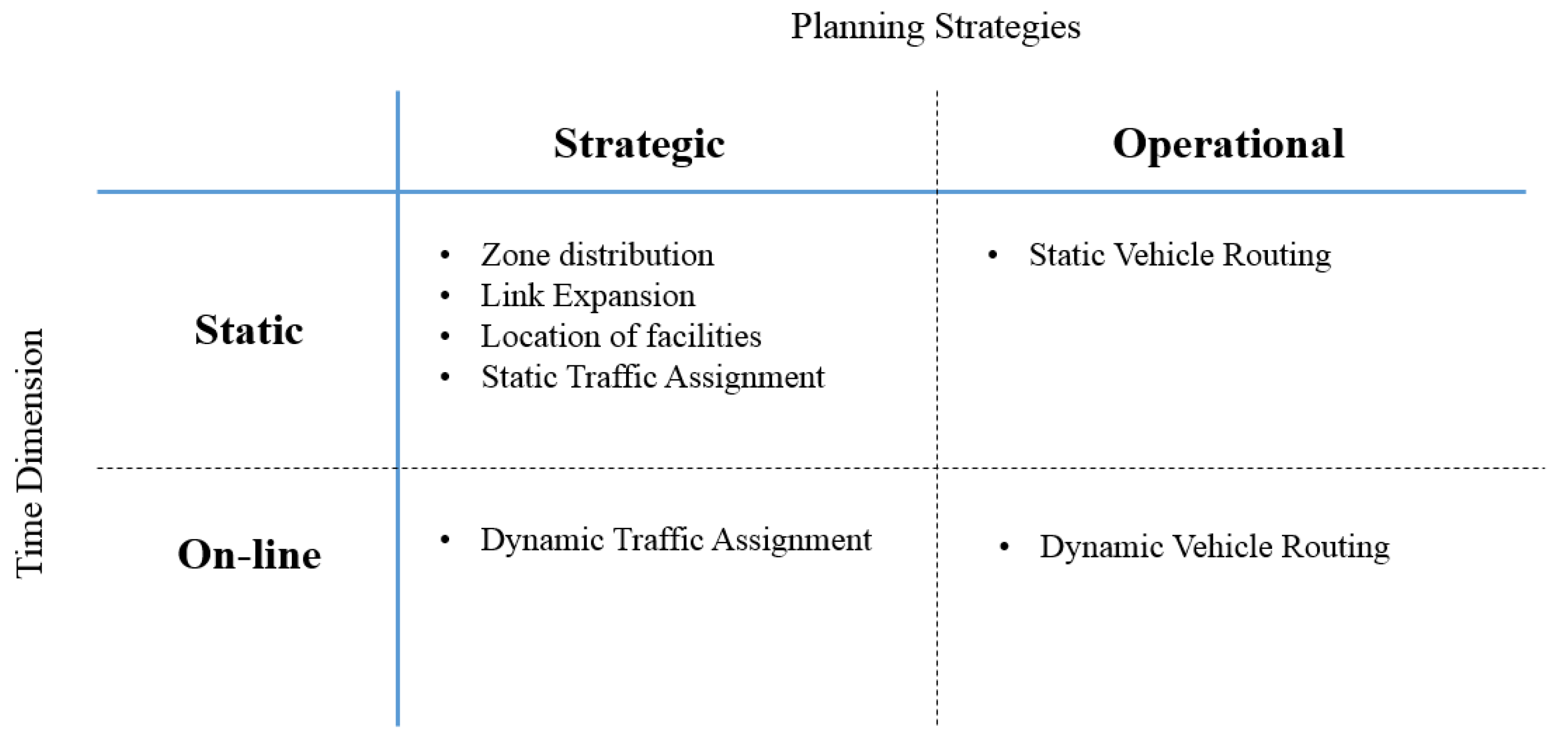
Figure 1.
Some of the operational research problems that can be considered when planning for urban design.
Figure 1.
Some of the operational research problems that can be considered when planning for urban design.

Figure 2.
Proposed framework for planning in smart cities.

Figure 3.
Steps involved in the k-means clustering approach adopted for zoning of the region. (A) Nodes in the region for positioning new buildings are identified a priori (i.e., circles); (B) centroids of zones to be created are placed randomly in the region (i.e., squares); (C) each node in the region is assigned to a centroid based on distance proximity (each node is numbered and assigned to a numbered centroid; matching displayed through the shading in the figure); (D) the location of the centroid is recalculated and new nodes are assigned/removed in response; (E) the final clusters are created.

Figure 4.
Solution approach adopted for the bilevel airport location model.

Figure 5.
Grids defined for piecewise linearisation of the BPR function.

Figure 6.
(A) Region examined in the case example; (B) available locations for placing buildings in the region.
Figure 6.
(A) Region examined in the case example; (B) available locations for placing buildings in the region.

Figure 7.
(A) Resulting zonal cluster where location nodes (in yellow) are grouped to the zone clusters (square); (B) Pattern matching between zones and allocated locations.
Figure 7.
(A) Resulting zonal cluster where location nodes (in yellow) are grouped to the zone clusters (square); (B) Pattern matching between zones and allocated locations.

Figure 8.
Transportation network of case example, where the numbered squares are the zones, and the arrows indicated the travel networks between the zones.
Figure 8.
Transportation network of case example, where the numbered squares are the zones, and the arrows indicated the travel networks between the zones.

Figure 9.
Box plot highlighting performance of the model proposed as instance size increases.

Figure 10.
(A) Solving time and (B) percentage (%) optimality of solution quality comparison between the genetic algorithm (GA), particle swarm optimisation (PSO) and the exact approach.
Figure 10.
(A) Solving time and (B) percentage (%) optimality of solution quality comparison between the genetic algorithm (GA), particle swarm optimisation (PSO) and the exact approach.

Figure 11.
(A) Pareto curve highlighting the trade-off between noise minimisation and carbon-equivalent emission minimisation; (B) Pareto curve highlighting the trade-off between noise minimisation and layout cost minimisation; (C) Pareto curve highlighting the trade-off between layout cost minimisation and carbon-equivalent emission minimisation.


Table 1.
Land-use distribution.
| Land Use | Zone Cluster | Location Nodes |
|---|---|---|
| Residential | 1 | 1, 2 |
| Residential | 2 | 3, 4 |
| Residential | 3 | 5, 6 |
| Mixed use | 4 | 7, 8 |
| Commercial | 5 | 11, 12 |
| Mixed use | 6 | 9, 10 |
| Commercial | 7 | 13, 14 |
| Industrial | 8 | 15, 16, 17, 18, 19 |
Table 2.
Building type and associated noise characteristics.
| Building Type | Maximum Noise Generated (dB(A)) | Noise Sensitivity Threshold (dB(A)) |
|---|---|---|
| Office | 70 | 70 |
| School | 80 | 55 |
| Residential | 75 | 60 |
| Hospital | 65 | 40 |
| Bus Stop | 85 | 75 |
| Factory | 85 | 75 |
Table 3.
Emission factors for each transportation mode analysed.
| Transportation Mode | |
|---|---|
| Car | 0.183 |
| Bus | 0.056 |
| Intercity Train | 0.041 |
Table 4.
Lexicographic optimisation with the order .
| Constructed Links | ||||
|---|---|---|---|---|
| 19,786 | 679 | 5,287,456 | All links | |
| 19,786 | 375 | 6,427,212 | All links | |
| 19,786 | 375 | 6,287,456 | All links |
Table 5.
Payoff table between all objective functions considered.
| Objective Functions | B1 = Layout Cost ($) | B2 = Noise (dB(A)) | |
|---|---|---|---|
| Min B1 | 3,825,976 | 679 | 131,115 |
| Min B2 | 8,786,432 | 276 | 131,115 |
| Min B3 | 10,321,452 | 679 | 19,786 |
© 2019 by the authors. Licensee MDPI, Basel, Switzerland. This article is an open access article distributed under the terms and conditions of the Creative Commons Attribution (CC BY) license (http://creativecommons.org/licenses/by/4.0/).
Share and Cite
MDPI and ACS Style
Hammad, A.W.; Akbarnezhad, A.; Haddad, A.; Vazquez, E.G. Sustainable Zoning, Land-Use Allocation and Facility Location Optimisation in Smart Cities. Energies 2019, 12, 1318. https://doi.org/10.3390/en12071318
AMA Style
Hammad AW, Akbarnezhad A, Haddad A, Vazquez EG. Sustainable Zoning, Land-Use Allocation and Facility Location Optimisation in Smart Cities. Energies. 2019; 12(7):1318. https://doi.org/10.3390/en12071318
Chicago/Turabian StyleHammad, Ahmed WA, Ali Akbarnezhad, Assed Haddad, and Elaine Garrido Vazquez. 2019. "Sustainable Zoning, Land-Use Allocation and Facility Location Optimisation in Smart Cities" Energies 12, no. 7: 1318. https://doi.org/10.3390/en12071318
Note that from the first issue of 2016, this journal uses article numbers instead of page numbers. See further details here.