New Design of a Supervised Energy Disaggregation Model Based on the Deep Neural Network for a Smart Grid


Abstract
:1. Introduction
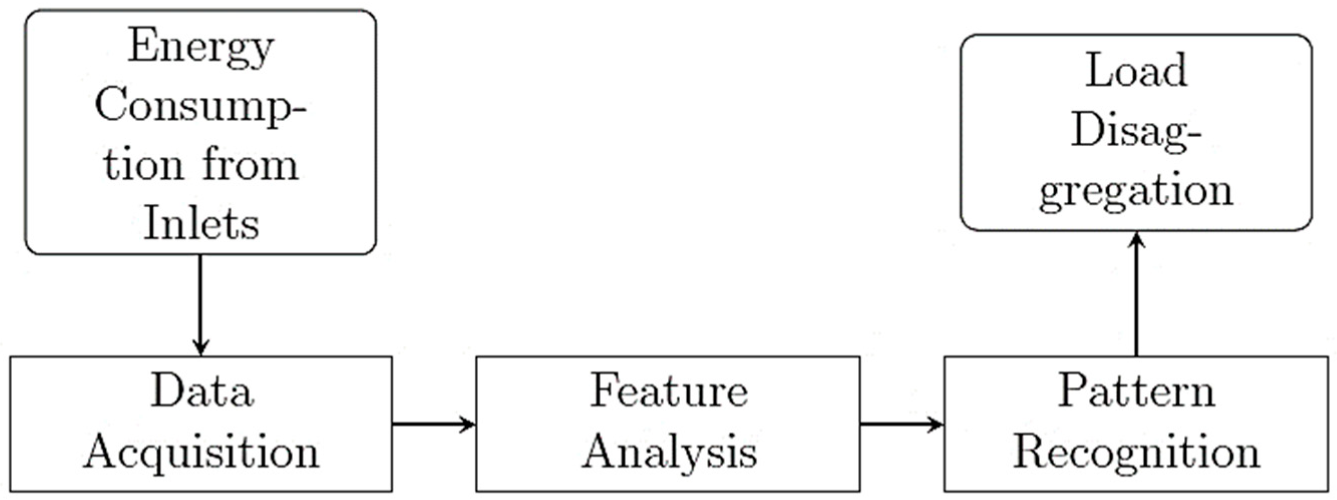
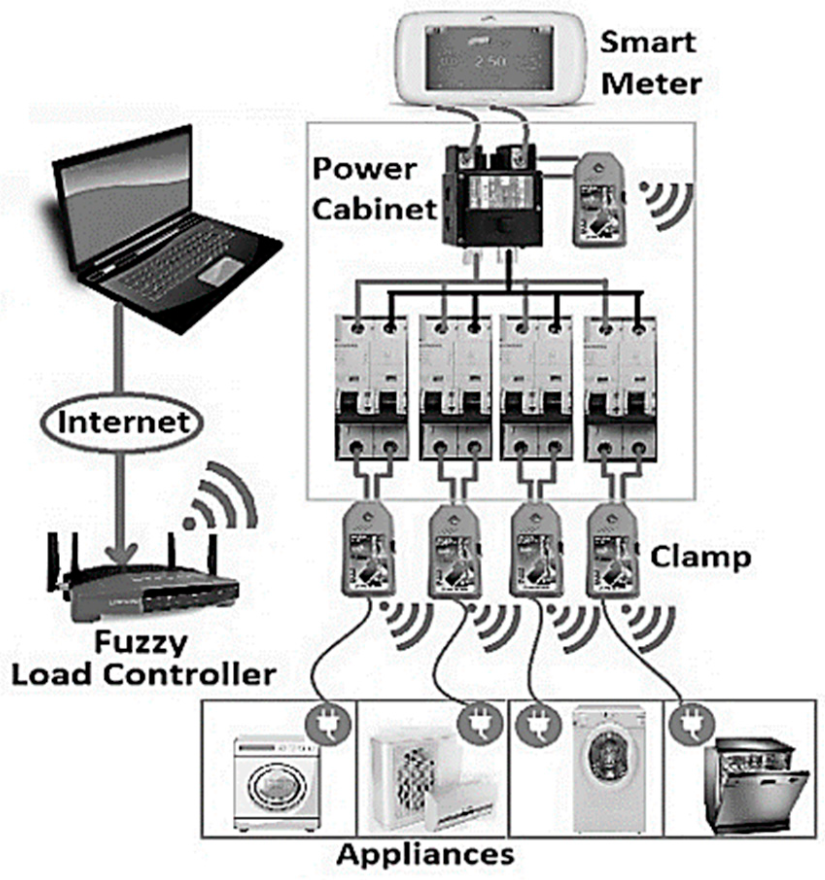
NILM Background
2. Learning Process and Error Function
3. Deep Learning
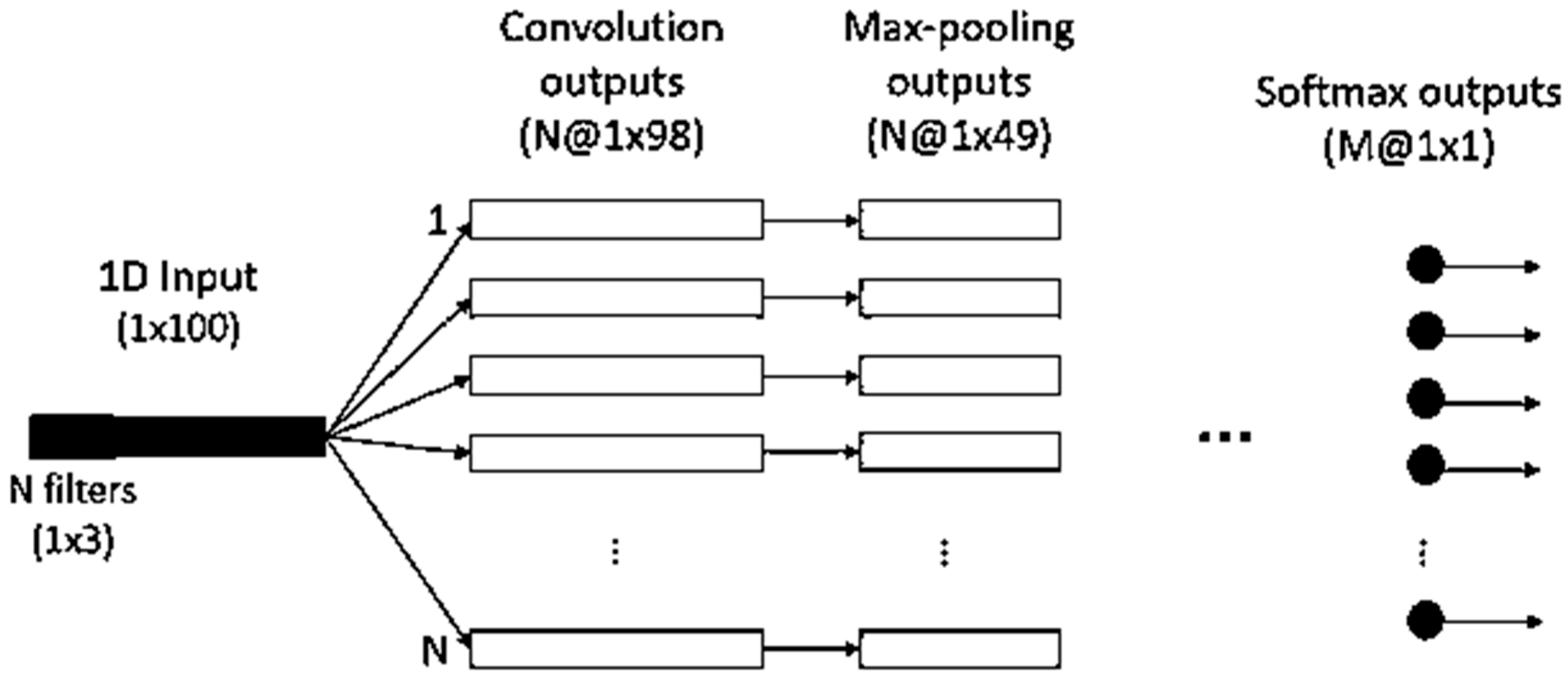
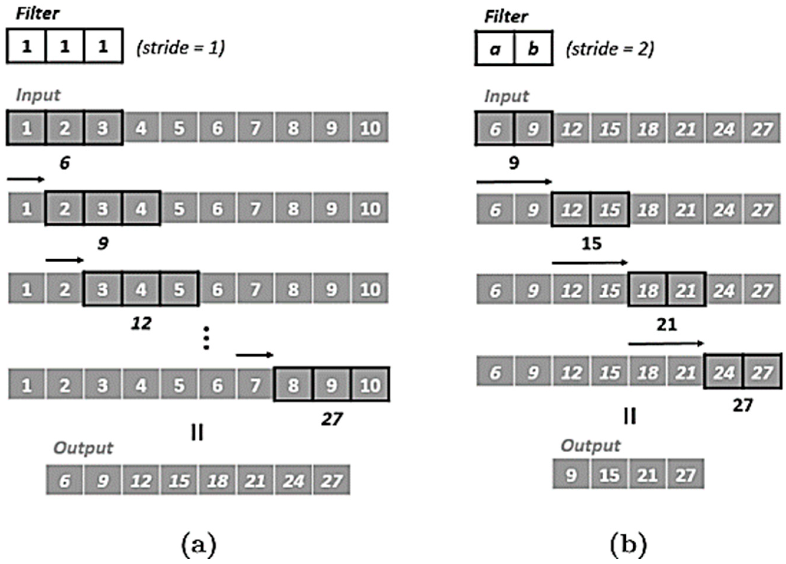
3.1. Convolutional Neural Networks
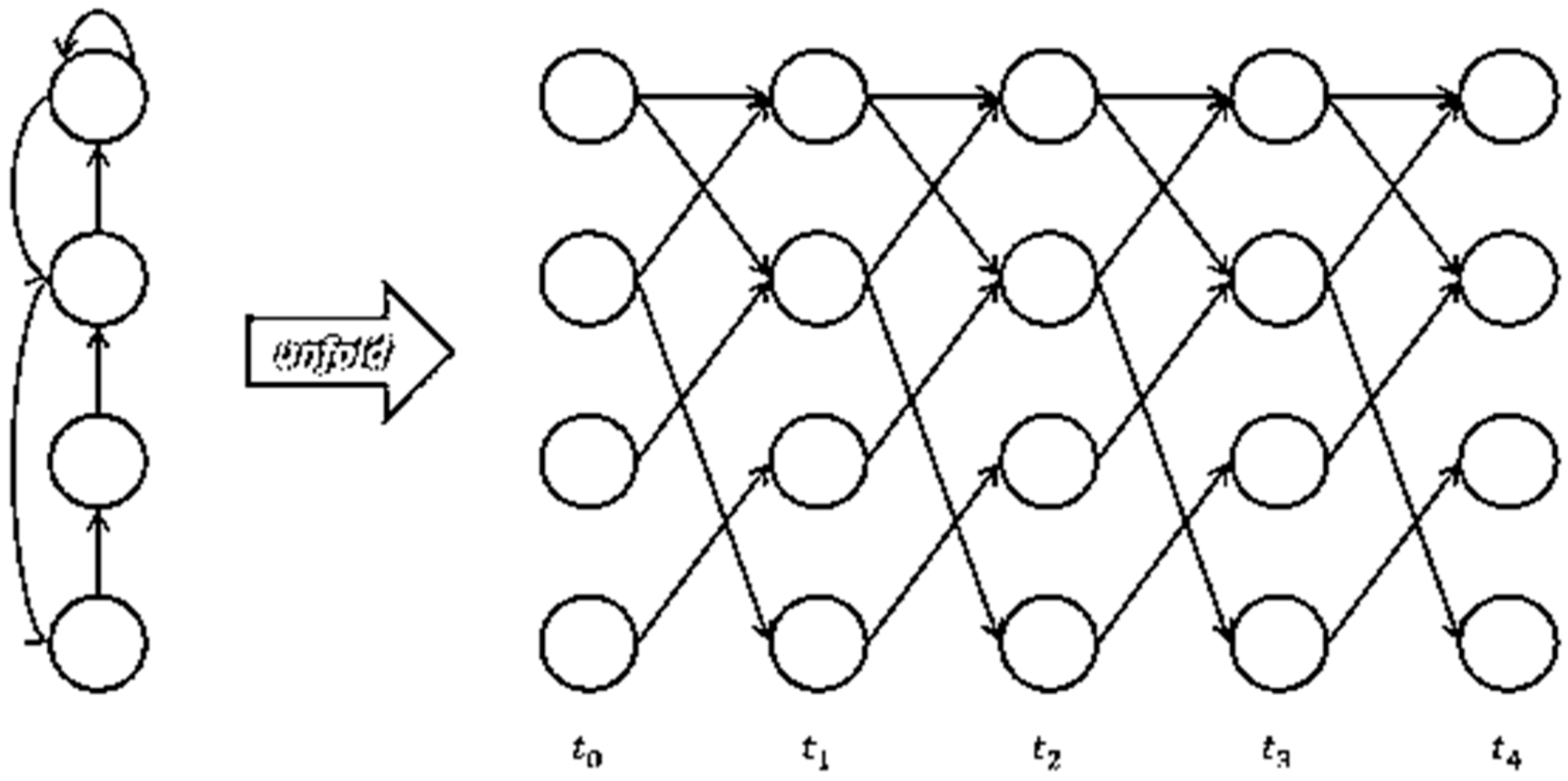
3.2. Recurrence Neural Networks
4. D CNN and RNN on NILM
4.1. REDD Dataset and Preprocessing
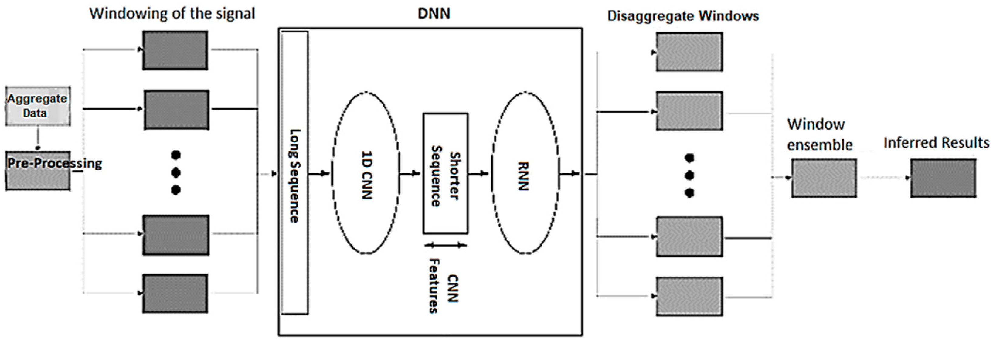
4.2. Combining CNN and RNN
4.3. Long Short-Term Memory (LSTM)
4.4. Metrics for Evaluating the NILM
- TP (total number of real positives): When both the device and ground truth are ON.
- FP (total number of fake positives): when the device is ON and ground truth is OFF.
- TN (total number of real negatives): when both the device and ground truth are OFF.
- FN (total number of fake negatives): when the device is OFF and ground truth is ON.
- P- Total number of positives on ground truth.
- N- Total number of negatives on ground truth.
4.4.1. Proportion of Total Energy Classified Correctly
4.4.2. Mean Normalized Error
4.4.3. Recall
4.4.4. Precision
4.4.5. Accuracy
4.4.6. F1 Score
4.4.7. Mean Square Error
4.4.8. Categorical Cross-Entropy
5. Houses not Seen During the Training for Testing
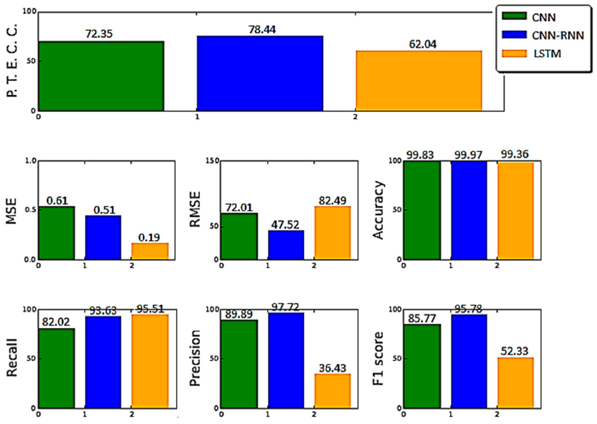
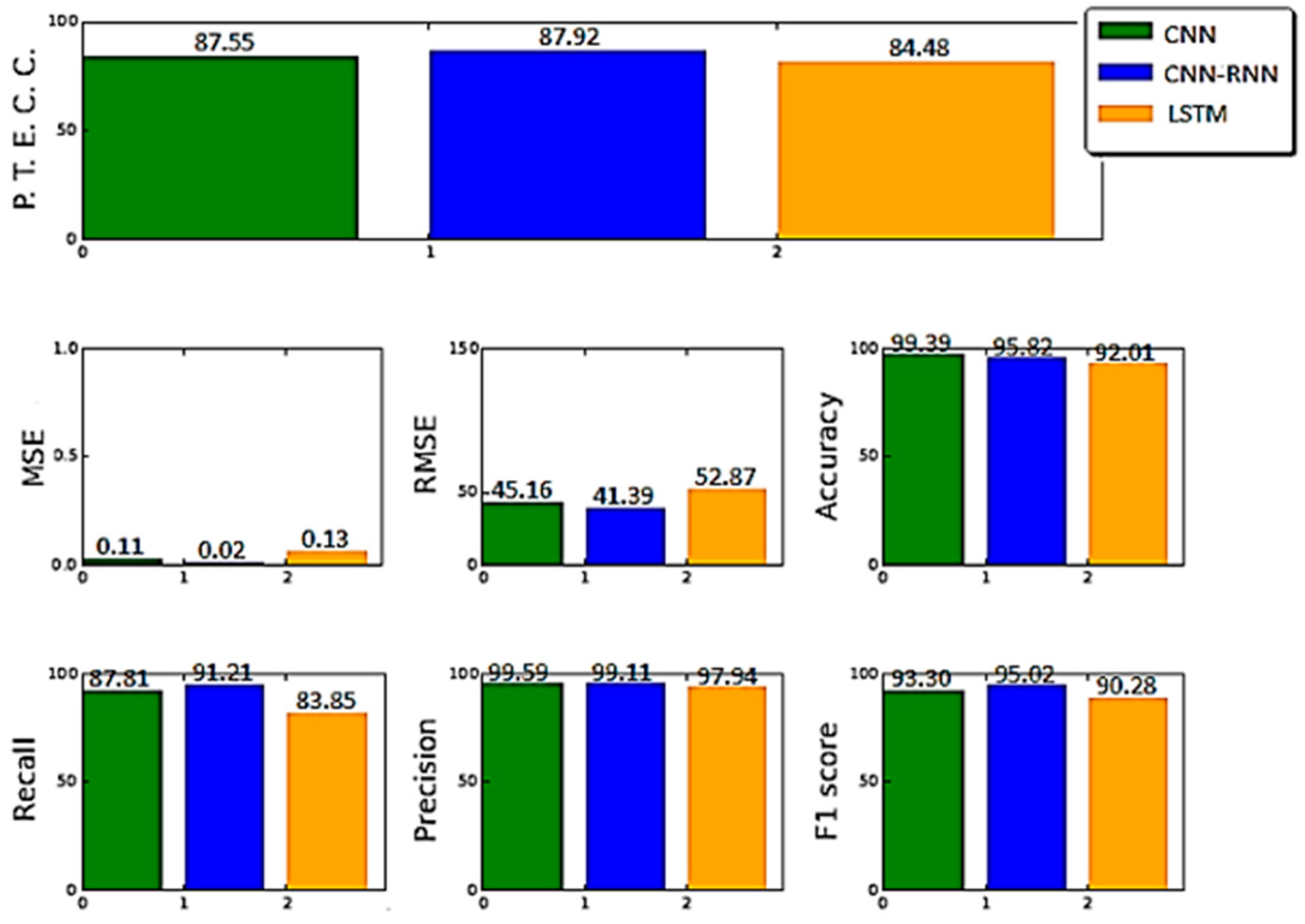
6. Results
- Implementation of DL in NILM and its potential for problem solving were examined.
- A combined method was introduced to show the approach of implementing DL methods using a small amount of real data.
7. Conclusions
8. Future Works
Author Contributions
Funding
Conflicts of Interest
References
- Faustine, A.; Mvungi, N.H.; Kaijage, S.; Michael, K. A survey on non-intrusive load monitoring methodies and techniques for energy disaggregation problem. arXiv, 2017; arXiv:1703.00785. [Google Scholar]
- Batra, N.; Singh, A.; Whitehouse, K. If you measure it, can you improve it? exploring the value of energy disaggregation. In Proceedings of the 2nd ACM International Conference on Embedded Systems for Energy-Efficient Built Environments, Seoul, Korea, 4–5 November 2015; pp. 191–200. [Google Scholar]
- Batra, N.; Singh, A.; Whitehouse, K. Gemello: Creating a detailed energy breakdown from just the monthly electricity bill. In Proceedings of the 22nd ACM SIGKDD International Conference on Knowledge Discovery and Data Mining, San Francisco, CA, USA, 13–17 August 2016; pp. 431–440. [Google Scholar]
- Zhong, M.; Goddard, N.; Sutton, C. Interleaved factorial non-homogeneous hidden Markov models for energy disaggregation. arXiv, 2014; arXiv:1406.7665. [Google Scholar]
- Reyes Lua, A.R. Location-aware Energy Disaggregation in Smart Homes. Master’s Thesis, Delft University of Technology, Delft, The Netherlands, 2015. [Google Scholar]
- Froehlich, J.; Larson, E.; Gupta, S.; Cohn, G.; Reynolds, M.; Patel, S. Disaggregated end-use energy sensing for the smart grid. IEEE Pervasive Comput. 2011, 10, 28–39. [Google Scholar] [CrossRef]
- Hart, G.W. Nonintrusive appliance load monitoring. Proc. IEEE 1992, 80, 1870–1891. [Google Scholar] [CrossRef]
- Barsim, K.S.; Streubel, R.; Yang, B. An approach for unsupervised non-intrusive load monitoring of residential appliances. In Proceedings of the 2nd International Workshop on Non-Intrusive Load Monitoring, Austin, TX, USA, 3 June 2014. [Google Scholar]
- Makonin, S.; Popowich, F.; Bajić, I.V.; Gill, B.; Bartram, L. Exploiting HMM sparsity to perform online real-time nonintrusive load monitoring. IEEE Trans. Smart Grid 2016, 7, 2575–2585. [Google Scholar] [CrossRef]
- Stankovic, V.; Liao, J.; Stankovic, L. A graph-based signal processing approach for low-rate energy disaggregation. In Proceedings of the 2014 IEEE Symposium on Computational Intelligence for Engineering Solutions (CIES), Orlando, FL, USA, 9–12 December 2014; pp. 81–87. [Google Scholar]
- do Nascimento, P.P.M. Applications of Deep Learning Techniques on NILM. Ph.D. Thesis, Universidade Federal do Rio de Janeiro, Rio de Janeiro, Brazil, 2016. [Google Scholar]
- Lowe, D.G. Object recognition from local scale-invariant features. In Proceedings of the ICCV, Corfu, Greece, 20–25 September 1999; p. 1150. [Google Scholar]
- Krizhevsky, A.; Sutskever, I.; Hinton, G.E. Imagenet classification with deep convolutional neural networks. In Proceedings of the Advances in Neural Information Processing Systems, Lake Tahoe, NV, USA, 3–6 December 2012; pp. 1097–1105. [Google Scholar]
- Graves, A.; Jaitly, N. Towards end-to-end speech recognition with recurrent neural networks. In Proceedings of the International Conference on Machine Learning, Beijing, China, 21–26 June 2014; pp. 1764–1772. [Google Scholar]
- Sutskever, I.; Vinyals, O.; Le, Q.V. Sequence to sequence learning with neural networks. In Proceedings of the Advances in Neural Information Processing Systems, Montreal, QC, Canada, 8–13 December 2014; pp. 3104–3112. [Google Scholar]
- Mnih, V.; Kavukcuoglu, K.; Silver, D.; Rusu, A.A.; Veness, J.; Bellemare, M.G.; Graves, A.; Riedmiller, M.; Fidjeland, A.K.; Ostrovski, G.; et al. Human-level control through deep reinforcement learning. Nature 2015, 518, 529. [Google Scholar] [CrossRef] [PubMed]
- Roos, J.G.; Lane, I.E.; Botha, E.C.; Hancke, G.P. Using neural networks for non-intrusive monitoring of industrial electrical loads. In Proceedings of the Conference Proceedings, 10th Anniversary. IMTC/94. Advanced Technologies in I & M, 1994 IEEE Instrumentation and Measurement Technolgy Conference (Cat. No. 94CH3424-9), Hamamatsu, Japan, 10–12 May 1994; pp. 1115–1118. [Google Scholar]
- Yang, H.T.; Chang, H.H.; Lin, C.L. Design a neural network for features selection in non-intrusive monitoring of industrial electrical loads. In Proceedings of the 2007 11th International Conference on Computer Supported Cooperative Work in Design, Melbourne, Australia, 26–28 April 2007; pp. 1022–1027. [Google Scholar]
- Google Colab Free GPU Tutorial. June 2018. Available online: https://medium.com/deep-learning-turkey/google-colab-free-gpu-tutorial-e113627b9f5d (accessed on 11 January 2018).
- Randles, B.M.; Pasquetto, I.V.; Golshan, M.S.; Borgman, C.L. Using the Jupyter notebook as a tool for open science: An empirical study. In Proceedings of the 2017 ACM/IEEE Joint Conference on Digital Libraries (JCDL), Toronto, ON, Canada, 19–23 June 2017; pp. 1–2. [Google Scholar]
- Torti, E.; Fontanella, A.; Musci, M.; Blago, N.; Pau, D.; Leporati, F.; Piastra, M. Embedded Real-Time Fall Detection with Deep Learning on Wearable Devices. In Proceedings of the 2018 21st Euromicro Conference on Digital System Design (DSD), Prague, Czech Republic, 29–31 August 2018; pp. 405–412. [Google Scholar]
- Movidius Announces Deep Learning Accelerator and Fathom Software Framework. Available online: https://developer.movidius.com/ (accessed on 8 January 2018).
- Zunnurain, I.; Maruf, M.; Rahman, M.; Shafiullah, G.M. Implementation of advanced demand side management for microgrid incorporating demand response and home energy management system. Infrastructures 2018, 3, 50. [Google Scholar] [CrossRef]
- Krishna, P.N.; Gupta, S.R.; Shankaranarayanan, P.V.; Sidharth, S.; Sirphi, M. Fuzzy Logic Based Smart Home Energy Management System. In Proceedings of the 2018 9th International Conference on Computing, Communication and Networking Technologies (ICCCNT), Bangalore, India, 10–12 July 2018; pp. 1–5. [Google Scholar]
- Kabalci, E.; Kabalci, Y. Introduction to Smart Grid Architecture. In Smart Grids and Their Communication Systems; Springer: Singapore, 2019; pp. 3–45. [Google Scholar]
- Mané, D. TensorBoard: TensorFlow’s Visualization Toolkit. 2015. Available online: https://github.com/tensorflow/tensorboard (accessed on 5 December 2017).
- Qian, S.; Liu, H.; Liu, C.; Wu, S.; San Wong, H. Adaptive activation functions in convolutional neural networks. Neurocomputing 2018, 272, 204–212. [Google Scholar] [CrossRef]
- Kotsiantis, S.B.; Zaharakis, I.; Pintelas, P. Supervised machine learning: A review of classification techniques. Emerg. Artif. Intell. Appl. Comput. Eng. 2007, 160, 3–24. [Google Scholar]
- Barsim, K.S.; Yang, B. Toward a semi-supervised non-intrusive load monitoring system for event-based energy disaggregation. In Proceedings of the 2015 IEEE Global Conference on Signal and Information Processing (GlobalSIP), Orlando, FL, USA, 14–16 December 2015; pp. 58–62. [Google Scholar]
- Rumelhart, D.E. Parallel distributed processing: Explorations in the microstructure of cognition. Learn. Intern. Represent. Error Propag. 1986, 1, 318–362. [Google Scholar]
- Richmond, C.D. Mean-squared error and threshold SNR prediction of maximum-likelihood signal parameter estimation with estimated colored noise covariances. IEEE Trans. Inf. Theory 2006, 52, 2146–2164. [Google Scholar] [CrossRef]
- Kalchbrenner, N.; Grefenstette, E.; Blunsom, P. A convolutional neural network for modelling sentences. In Proceedings of the 52nd Annual Meeting of the Association for Computational Linguistics, Baltimore, Maryland, 23–25 June 2014. [Google Scholar]
- Wolfe, J.; Jin, X.; Bahr, T.; Holzer, N. Application of softmax regression and its validation for spectral-based land cover mapping. The International Archives of Photogrammetry. Remote Sens. Spat. Inf. Sci. 2017, 42, 455. [Google Scholar]
- Ullah, A.; Ahmad, J.; Muhammad, K.; Sajjad, M.; Baik, S.W. Action recognition in video sequences using deep bi-directional LSTM with CNN features. IEEE Access 2018, 6, 1155–1166. [Google Scholar] [CrossRef]
- Glorot, X.; Bordes, A.; Bengio, Y. Deep sparse rectifier neural networks. In Proceedings of the Fourteenth International Conference on Artificial Intelligence and Statistics, Fort Lauderdale, FL, USA, 11–13 April 2011; pp. 315–323. [Google Scholar]
- Sundermeyer, M.; Ney, H.; Schlüter, R. From feedforward to recurrent LSTM neural networks for language modeling. IEEE/ACM Trans. Audio, Speech Lang. Process. 2015, 23, 517–529. [Google Scholar] [CrossRef]
- Squartini, S.; Hussain, A.; Piazza, F. Attempting to reduce the vanishing gradient effect through a novel recurrent multiscale architecture. In Proceedings of the International Joint Conference on Neural Networks, Portland, OR, USA, 20–24 July 2003; Volume 4, pp. 2819–2824. [Google Scholar]
- Kelly, J.; Knottenbelt, W. Neural NILM: Deep neural networks applied to energy disaggregation. In Proceedings of the 2nd ACM International Conference on Embedded Systems for Energy-Efficient Built Environments, Seoul, Korea, 4–5 November 2015; pp. 55–64. [Google Scholar]
- Kolter, J.Z.; Johnson, M.J. REDD: A public data set for energy disaggregation research. In Proceedings of the Workshop on Data Mining Applications in Sustainability (SIGKDD), San Diego, CA, USA, 21–24 August 2011; Volume 25, pp. 59–62. [Google Scholar]
- Hochreiter, S.; Schmidhuber, J. Long short-term memory. Neural Comput. 1997, 9, 1735–1780. [Google Scholar] [CrossRef] [PubMed]
- Sherstinsky, A. Fundamentals of Recurrent Neural Network (RNN) and Long Short-Term Memory (LSTM) Network. arXiv, 2018; arXiv:1808.03314. [Google Scholar]
- Gers, F.A.; Schraudolph, N.N.; Schmidhuber, J. Learning precise timing with LSTM recurrent networks. J. Mach. Learn. Res. 2002, 3, 115–143. [Google Scholar]
- Gers, F.A.; Schmidhuber, J.; Cummins, F. Learning to Forget: Continual prediction with LSTM. In Proceedings of the 9th International Conference on Artificial Neural Networks: ICANN ’99, Edinburgh, UK, 7–10 September 1999. [Google Scholar]
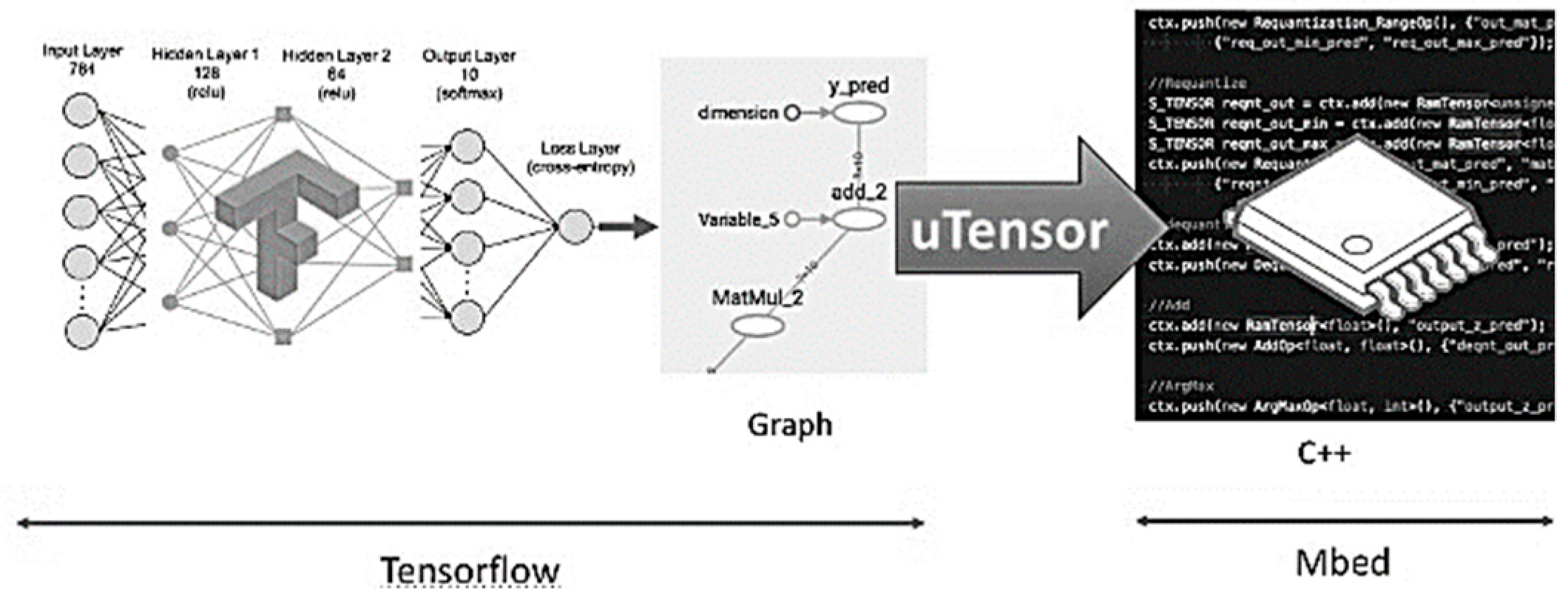
- Available online: https://github.com/uTensor/uTensor (accessed on 3 January 2018).


| Device | Training | Testing |
|---|---|---|
| Microwave | 1, 3 | 2 |
| Dish washer | 1, 3 | 2, 4 |
| Refrigerator | 1, 3 | 2, 6 |
© 2019 by the authors. Licensee MDPI, Basel, Switzerland. This article is an open access article distributed under the terms and conditions of the Creative Commons Attribution (CC BY) license (http://creativecommons.org/licenses/by/4.0/).
Share and Cite
ÇAVDAR, İ.H.; FARYAD, V. New Design of a Supervised Energy Disaggregation Model Based on the Deep Neural Network for a Smart Grid. Energies 2019, 12, 1217. https://doi.org/10.3390/en12071217
ÇAVDAR İH, FARYAD V. New Design of a Supervised Energy Disaggregation Model Based on the Deep Neural Network for a Smart Grid. Energies. 2019; 12(7):1217. https://doi.org/10.3390/en12071217
Chicago/Turabian StyleÇAVDAR, İsmail Hakkı, and Vahid FARYAD. 2019. "New Design of a Supervised Energy Disaggregation Model Based on the Deep Neural Network for a Smart Grid" Energies 12, no. 7: 1217. https://doi.org/10.3390/en12071217
APA StyleÇAVDAR, İ. H., & FARYAD, V. (2019). New Design of a Supervised Energy Disaggregation Model Based on the Deep Neural Network for a Smart Grid. Energies, 12(7), 1217. https://doi.org/10.3390/en12071217