A Model for Multi-Energy Demand Response with Its Application in Optimal TOU Price

Abstract

With the generalization of the integrated energy system (IES) on the demand side, multi-energy users may participate in a demand response (DR) program based on their flexible consumption of energy. However, since users could choose using alternative energy or transfer energy consumption to other time periods, obtaining response characteristics of this type of DR usually appears more complicated than traditional single-energy DR. To obtain the response characteristic, a response model for multi-energy DR, which reflects the relations between electricity (gas) response and time-of-use (TOU) electric prices, is proposed. The model is characterized by several coefficients which are associated with electric and heat efficiency. The model is obtained through the derivation process of optimizing user’s energy-using problem. Then, as a typical application of the response model, the TOU electric pricing for multi-energy users is able to be formulated by an interior point algorithm after giving the Kuhn-Tucker conditions of the optimal problem. Typical results of the optimal TOU pricing are further illustrated through the formulation on a PJM five-bus test system. It demonstrates that optimal TOU pricing can be effectively pre-calculated by the utility company using the proposed response model.

1. Introduction

With the generalization of energy connection on the demand side, the integrated energy system (IES) is becoming widely used for large users such as industrial users, which need both electricity and heat for industrial production [1]. The energy options tend to be more diverse, and the energy consumption is more flexible due to the adoption of IES. This provides the multi-energy users with sufficient conditions for the generation of demand response (DR) [2]. According to the price signals, multi-energy users could regulate the operation mode of IES to optimize the purchase of input energy, thus forming the response to energy price. For instance, when faced with the situation where electricity price is higher than gas price, multi-energy users tend to purchase more gas than electricity by improving the utilization of gas devices instead of electric devices. This type of DR, which can be regarded as a derived product of energy connection [3], has advantages of less impact on users’ comfort, higher motivation for response, larger response potential, and lower uncertainty compared with single-energy DR such as traditional electric DR. As a novel type of integrated energy DR, multi-energy DR will play an important role in interacting with the electric grid under the new energy circumstances. Aiming at a better application of multi-energy DR, the response characteristics need to be learned and addressed.

Researchers around the world have devoted much effort to study response characteristics of electric DR through various approaches such as establishing the elasticity matrix of electric demand [4,5,6,7], fitting load transferring curve [8], and so on. However, multi-energy DR is still in the recognizing stage, and there is not sufficient research on the response mechanism and response model until now. The research work, which focuses on the response behavior of multi-energy resources—such as micro-combined cooling heat and power (CCHP) systems for residential use [9], the flexible electric-heat system [10], electric-heat load (heat pumps) [11], and energy-hub for home [3,12] is progressing gradually. Besides, some work in the literature refers to the response characteristics of electric-heat load participating in ancillary services such as frequency or voltage regulation [13,14,15,16]. Based on the summary of these multi-energy resources, reference [17] proposed the concept of integrated energy demand response and analyzed the response potential of IES. Moreover, references [3,18] provides frameworks of DR program for multi-energy users to realize more active interactions with the outer energy grid. However, the research above still lacks a tangible response model, which is required to analyze response mechanisms in consideration of energy price, system configuration, and other factors. Whereas for a better application of multi-energy DR, a clear response model, which reflects the relations of response amount and energy prices explicitly, needs to be proposed as the basis of the application.

Since at least two types of loads are coupled in IES, the response characteristic is closely associated with such various factors as the parameters of energy conversion, storage devices, and multi-energy prices. Therefore, in order to establish a response model, the response mechanism, which depends on the system configuration and load conditions, needs to be analyzed clearly and explicitly for multi-energy DR. To address this challenge, this paper analyzes the energy flows proceeding from the IES’ configuration qualitatively, and derives a quantitative model responding to the time-of-use (TOU) electric price and the constant gas price for the industrial multi-energy user equipped with a typical electric-heat system. Moreover, optimal pricing for multi-energy users is presented as a typical application with the proposed model. The contributions of this paper are summarized as follows:

(1) Proposing a feasible and analytical way of establishing a response model for multi-energy DR, different from electric DR;

(2) specifying an explicit and uniform response model in the TOU electric price scheme and determining its influenced coefficients;

(3) avoiding a complex computation of the bi-level nonlinear optimization, which is usually difficult to solve, for making a pricing strategy for the multi-energy users.

The rest of this paper is organized as follows. The modeling for multi-energy user’s response in the TOU price scheme is introduced in Section 2. In Section 3, an optimal TOU price problem is formulated as an optimization problem based on the proposed response model. Numerical examples are presented in Section 4. Section 5 presents the summary and conclusion.

2. Modeling for Multi-Energy User’s Response in TOU Price

2.1. Energy Flows of Multi-Energy DR in TOU Price

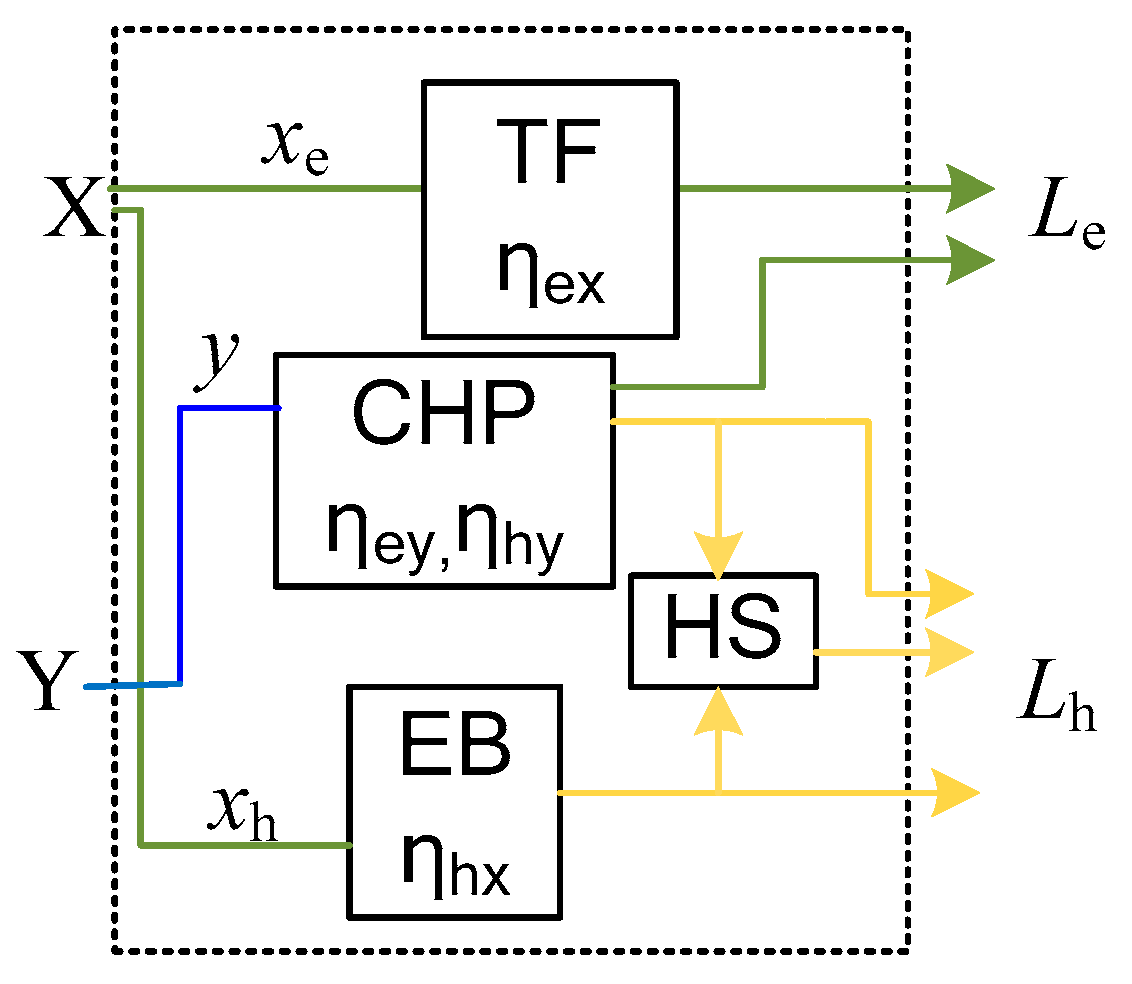
For the multi-energy users applied with IES, there are at least two types of input energy (electricity, gas, etc.) as well as at least two types of output load (electricity, heat, cooling, etc.) [19]. The IES determines a specified conversion relation between input energy and output load. Taking an electric-heat system [20] with combined heat and power (CHP), electric boiler (EB), and heat storage (HS) as an example, which is illustrated in Figure 1, the input energy is electricity (represented as X) and gas (represented as Y), and the output is electricity load (represented as L_e) and heat load (represented as L_h). This system configuration makes it possible that electricity load or heat load could be satisfied with either electricity or gas. A multi-energy user could adjust the output of conversion devices (CHP, EB) to alter the purchase amount of electricity and gas from the outer energy grid. It means that the input amount could be altered through energy substitution on the premise of maintaining constant loads of IES. Besides, if the day-ahead energy prices are posted to users, users could also utilize heat storage devices to make it possible for heat load transferring among different time slots for one day. Thus, the input energy amount for meeting heat load could be transferred from one moment to others within a day. In other words, the multi-energy user has more options for energy consumption, including both energy substitution and energy transfer. Therefore, the response characteristic of multi-energy DR tends to be more flexible than the single-energy DR.

Commonly for the electric-heat system in Figure 1, the input-output relations [21] could be characterized as a matrix equation in Equation (1).

$$\left[\begin{array}{c}{L}_e\\ L_h\end{array}\right]=\left[\begin{array}{ccc}\begin{array}{c}{\eta }_{ex}\\ 0\end{array}& \begin{array}{c}0\\ {\eta }_{hx}\end{array}& \begin{array}{c}{\eta }_{ey}\\ {\eta }_{hy}\end{array}\end{array}\right]\left[\begin{array}{c}{x}_e\\ x_h\\ \phi (y)\end{array}\right]$$

(1)

where x_e, x_h are corresponding to the purchase of electricity to satisfy electricity and heat load, respectively; y is the purchase of gas; η_ex, η_hx are electric and heat efficiency of electric devices, respectively (TF, EB); φ(y) is the output function of CHP (assumed as a quadratic function φ(y) = $\sqrt{my-n}$, m > 0, n ≥ 0 in this paper); η_ey, η_hy are the electric and heat efficiency of a gas device, respectively (CHP). For the cyclic utilization of HS, the total storage amount and release amount of heat should be equal in a day. Since HS is able to transfer heat load for one day, the total output of heat from CHP and EB through one day is supposed to be a constant value. The objective of the user is to minimize the purchase cost of input energy for one day, let z_t = $\sqrt{m{y}_t-n}$, the optimization problem can be written as

$$\min f={\displaystyle \sum _{t=1}^T\left[a_t(x_{e,t}+x_{h,t})+b_t\frac{z_t^2}{m}-\frac{n{b}_t}{m}\right]}$$

(2)

$$s.t. h: {\displaystyle \sum _{t=1}^T\left({\eta }_{hx}{x}_{h,t}+{\eta }_{hy}{z}_t\right)=L_{h,0}}$$

(3)

$${\eta }_{ex}{x}_{e,t}+{\eta }_{ey}{z}_t=L_{e,t}, \forall t$$

(4)

$$\begin{array}{cc}\begin{array}{l}{g}_1:x_{e,t}\ge 0, x_{h,t}\ge 0,z_t\ge 0\\ g_2:x_{e,t}\le x_{e,max},x_{h,t}\le x_{h,max},z_t\le \sqrt{m{y}_{max}-n}\end{array}& , \forall \end{array}t$$

(5)

In Equation (2), a_t, b_t are corresponding to electric and gas price at time slot t, T represents the number of time intervals; Constraint (3) means that the sum of heat load on an entire day is restricted by a constant value L_h,0; Constraint (4) is the equality constraint of electricity load in each time interval; Constraint (5) is the upper and lower limits of energy purchase for each device’s input. x_e,max, x_h,max, y_max are corresponding to the maximum input of TF, EB, and CHP, respectively. Note that, to simplify analysis of this example, we only present the most important constraints.

In this paper, the response characteristic in the TOU price scheme is mainly discussed. Hence, 24 hours in a day could be classified in three periods according to load level: peak, valley, and flat hours. The response amount of a single-energy user in the TOU scheme is determined by the price differences between peak, flat, and valley hours. Since the electricity amount can be transferred from peak hours to flat and valley hours, the reduction amount in peak hours could be deemed to be approximately equal to the increasing amount in flat and valley hours. However, the response characteristic of multi-energy DR, which could result from either substitution among electricity, gas, or the energy transfer among three time periods, is obviously more complicated. The analysis is presented as follows. In the following part, the peak, valley, and flat hours are represented as subscripts p, v, and f, respectively.

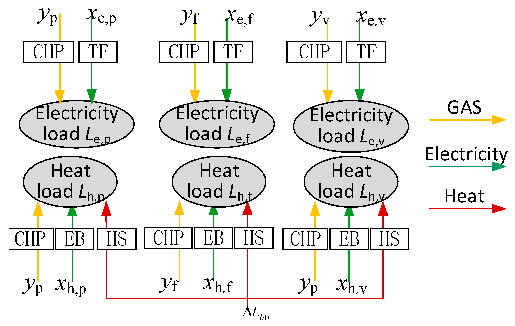
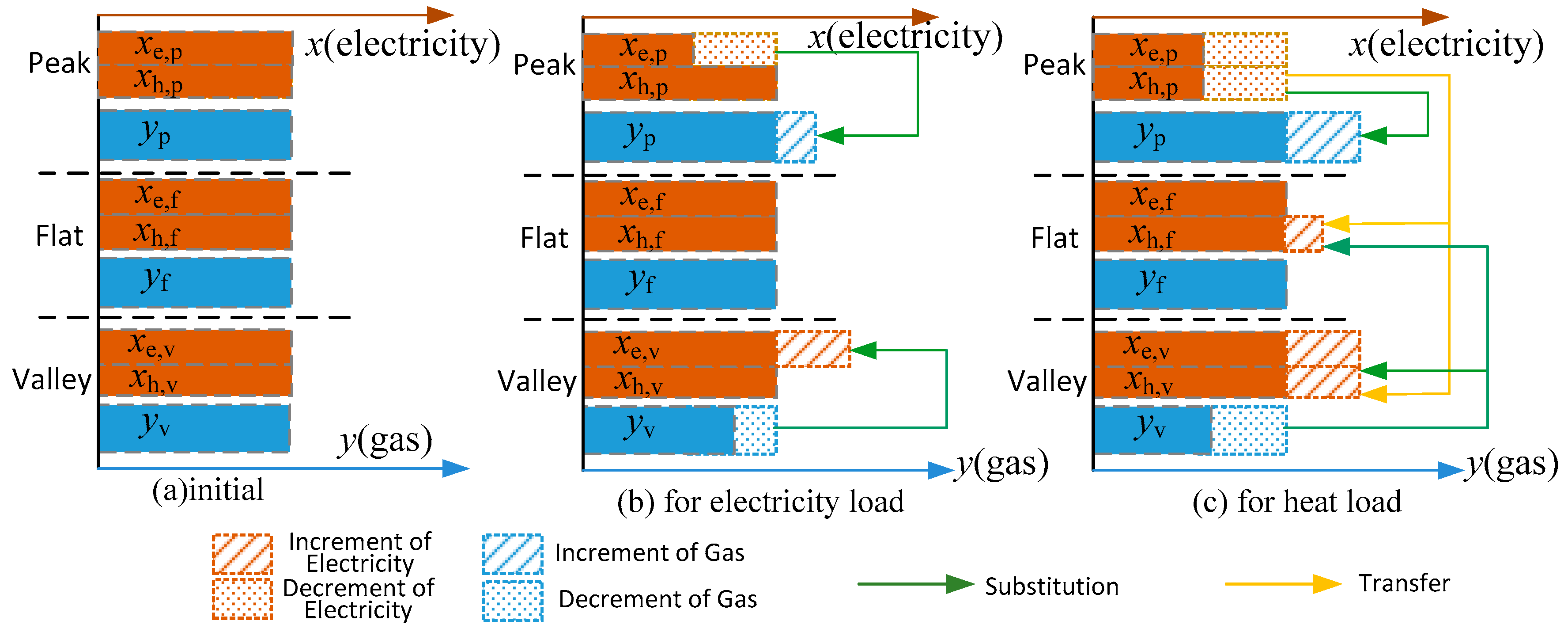
For the purpose of a comprehensive understanding of energy flow, the options of meeting electricity and the heat load at each period are illustrated in Figure 2. Electricity load at each period is independent, whereas heat load at each period is coupled due to the HS. Resorting to Figure 2, the energy flow for the process of the first implementation of TOU price scheme is more easily analyzed, as depicted in Figure 3. Figure 3a presents the initial state of energy consumption before the implementation of the TOU price scheme. The initial consumption amount is considered the same for three periods. After the implementation of TOU, the consumption amount would differ from Figure 3a. Energy flows will be analyzed from the views of IES’ electricity load and heat load, which are illustrated in Figure 3b,c, respectively.

Firstly, Figure 3b presents the energy flow due to the restriction of electricity load. According to Constraint (4), electricity load L_e,t is independent among three periods. It means that electricity purchase x_e,t for electricity load is simply restricted with gas purchase y_t at each time slot t. Therefore, with the higher price in peak hours, the electricity purchase x_e,p for electricity load in peak hours would decrease, leading to an increment of gas purchase y_p in peak hours. This indicates that the substitution between electricity and gas happens in the process of meeting electricity load. The relation is similar in valley hours.

Then Figure 3c presents the energy flow due to the restriction of heat load. According to Constraint (3) of heat load, the total amount of heat load is constant, i.e., $\Delta L_{h,0}=0$, and then Constraint (3) can be transformed as Constraint (6), which illustrates that the variation of electricity purchase for heat load is associated with the variations of gas purchase in the whole day.

$$({\displaystyle \sum _{t\in T_p}\Delta z_t}+{\displaystyle \sum _{t\in T_f}\Delta z_t}+{\displaystyle \sum _{t\in T_v}\Delta z_t}){\eta }_{hy}+({\displaystyle \sum _{t\in T_p}\Delta x_{\mathrm{h},t}}+{\displaystyle \sum _{t\in T_f}\Delta x_{\mathrm{h},t}}+{\displaystyle \sum _{t\in T_v}\Delta x_{h,t}}){\eta }_{hx}=0$$

(6)

As depicted in Figure 3c, due to the higher electric peak price, the electricity for heat load x_h,p would transfer from peak hours to flat and valley hours. Besides, part of x_h,p would be substituted into the amount of gas purchase y_p, since y_p has increased due to Constraint (4). Similarly, gas purchase y_v in valley hours would decrease resulted from Constraint (4), and also would be substituted into the increasing electricity for heat load x_h,v, x_h,f.

Overall, with the coupling device (CHP) in IES, the coupling of different loads makes the substitution of the two-input energy more complicated. Meanwhile, the introduction of flexible storage device makes energy purchase possible to transfer among time periods, leading to multi-direction energy flow. For example, constituted with the response amount of electricity purchase in flat hours, there are both transferring component from electricity purchase in peak hours and substituted component from gas purchase in valley hours. After all, the quantity of these components depends on price differences among periods, which will be derived in the following part.

2.2. Modeling of the Response Characteristics of Multi-Energy DR in TOU Price

The energy flow in IES has been analyzed qualitatively in Section 2.1. The mathematical model of multi-energy DR will be drawn through the derivation of the aforementioned optimizing problem. Firstly, substituting Constraint (4) into (2), the objective function is converted as

$$min f={\displaystyle \sum _{t=1}^T\left[a_t(x_{h,t}+\frac{L_{e,t}-{\eta }_{ey}{z}_t}{{\eta }_{ex}})+b_t\frac{z_t^2}{m}-\frac{n{b}_t}{m}\right]}.$$

(7)

In Constraint (5), the upper limit of z_t is converted as $z_t\le z_{max}$ ($z_{max}=min(\sqrt{m{y}_{max}-n},L_{e,t}{/\eta }_{ey})$). The decision variables are q = [x_h,1,…, x_h,T, z₁,…, z_T]^T. Since the Hessian matrix of f is positive and semi-definite, this problem can be regarded as convex. Hence, the optimal solution q^* certainly meets the Kuhn-Tucker Conditions (8), which means the K-T point (with use of the superscript * to represent) is the global optimum.

$$\{\begin{array}{l}\nabla f(q^{\ast })-{\lambda }^{\ast }\nabla h(q^{\ast })-{\displaystyle \sum _{t=1}^T{\mu }_{1t}^{\ast }}\nabla g_{1,t}(q^{\ast })+{\displaystyle \sum _{t=1}^T{\mu }_{2t}^{\ast }\nabla g_{2,t}(q^{\ast })=0}\\ {\mu }_{1t}^{\ast }{q}^{\ast }=0 , {\mu }_{2t}^{\ast }(q^{\ast }-q_{\max })=0, {\mu }_{1t}^{\ast }\ge 0, {\mu }_{2t}^{\ast }\ge 0, {\mu }_{1t}^{\ast }{\mu }_{2t}^{\ast }=0, \forall t\end{array}$$

(8)

where $\nabla f={[a_1,\dots ,a_T,\frac{2b_1}{m}{z}_1-a_1\frac{{\eta }_{ey}}{{\eta }_{ex}},\dots ,\frac{2b_T}{m}{z}_T-a_T\frac{{\eta }_{ey}}{{\eta }_{ex}}]}^T$, $\nabla h={[{\eta }_{hx},\dots ,{\eta }_{hx},{\eta }_{hy},\dots ,{\eta }_{hy}]}^T$.

In this paper, the electric prices in peak, valley, and flat hours are represented as a_p, a_v, and a_f. Since the TOU price mechanism has not been established in the gas market, the gas price is assumed as a constant (b₀ here) for one day. To establish Conditions (8), the value of either μ_1t or μ_2t could not be zero, which means the constraints of the upper or lower limit would make sense so that in valley hours, x_h,t^* = x_h,max, $t\in T_v$, and in peak hours, x_h,t^* = 0, $t\in T_p$. Since the flat price a_f is a middle price, the dual variables μ_1,t, μ_2,t ($t\in T_f$) are zero, and the Lagrangian multiplier λ^* is $a_f/{\eta }_{hx}$. Thus, in flat hours, 0 < x_h.t^* < x_h,max, $t\in T_f$. Besides, the optimum of intermediate variable z_t is obtained.

$$z_t{}^{\ast }=min\left(\frac{a_f{\eta }_{hy}m}{2b_0{\eta }_{hx}}+\frac{a_t{\eta }_{ey}m}{2b_0{\eta }_{ex}},z_{max}\right), t\in T_p{,T}_f{,T}_v$$

(9)

From Equation (9), z_t would be restricted by the capacity of CHP if electric price a_f, a_t rises to overtop. In this situation, z_t would not increase with the electric price any more, which means the response amount becomes saturated. To simplify the analysis, the variation of electricity prices is set within a certain range to avoid the response amount being saturated. Substituting those variables above into Constraint (3), electricity purchase for heat load in flat hours is obtained by Equation (10).

$$x_{h,t}{}^{\ast }=\frac{L_{h,0}}{8{\eta }_{hx}}-x_{h,max}-\frac{{m\eta }_{hy}}{{8\eta }_{hx}}{\displaystyle \sum _{t\in T_p{,T}_f{,T}_v}^{}\left(\frac{a_f{\eta }_{hy}}{2b_0{\eta }_{hx}}+\frac{a_t{\eta }_{ey}}{2b_0{\eta }_{ex}}\right)}, t\in T_f$$

(10)

From Equation (4), electricity purchase for electricity load at each time slot is obtained as

$$z_t{}^{\ast }=min\left(\frac{a_f{\eta }_{hy}m}{2b_0{\eta }_{hx}}+\frac{a_t{\eta }_{ey}m}{2b_0{\eta }_{ex}},z_{max}\right), t\in T_p{,T}_f{,T}_v.$$

(11)

Then, based on these demand Functions (9)–(11), the response amount is able to be obtained. During the sth time to implement TOU price scheme, the variations $\Delta x_{e,s,t}$, $\Delta x_{h,s,t}$, $\Delta z_{s,t}$ are defined as response amount at time slot t in the sth implementation. The variation of the electric price at time slot t is represented as $\Delta a_{s,t}$. From Functions (9)–(11), the response amount is easily obtained by Functions (12)–(14).

$$\Delta z_{s,t}=\left(\frac{{\eta }_{hy}}{{\eta }_{hx}}\Delta a_{s,f}+\frac{{\eta }_{ey}}{{\eta }_{ex}}\Delta a_{s,t}\right)\frac{m}{2b_0}, t\in T_p,T_f,T_v$$

(12)

$$\Delta x_{e,s,t}=-\frac{m{\eta }_{ey}}{{\eta }_{ex}}\left(\frac{{\eta }_{hy}}{{\eta }_{hx}}\Delta a_{s,f}+\frac{{\eta }_{ey}}{{\eta }_{ex}}\Delta a_{s,t}\right)\frac{1}{2b_0}, t\in T_p,T_f,T_v$$

(13)

$$\Delta x_{h,s,t}=0, t\in T_p; \Delta x_{h,s,t}=0, t\in T_v$$

(14)

$$\Delta x_{h,s,t}=-\frac{{\eta }_{hy}}{{\eta }_{hx}}\left(\frac{3{\eta }_{hy}}{{\eta }_{hx}}\Delta a_{s,f}+\frac{{\eta }_{ey}}{{\eta }_{ex}}(\Delta a_{s,p}+\Delta a_{s,v}+\Delta a_{s,f})\right)\frac{m}{2b_0}, t\in T_f$$

(15)

Finally, the electricity response $\Delta x_{s,t}$ at time slot t can be drawn from the sum of $\Delta x_{e,s,t}$ and $\Delta x_{h,s,t}$.

$$\Delta x_{s,t}=\{\begin{array}{l}-\frac{{\eta }_{ey}}{{\eta }_{ex}}\left(\frac{{\eta }_{hy}}{{\eta }_{hx}}\Delta a_{s,f}+\frac{{\eta }_{ey}}{{\eta }_{ex}}\Delta a_{s,p}\right)\frac{m}{2b_0}, t\in T_p\\ -\frac{{\eta }_{ey}}{{\eta }_{ex}}\left(\frac{{\eta }_{hy}}{{\eta }_{hx}}\Delta a_{s,f}+\frac{{\eta }_{ey}}{{\eta }_{ex}}\Delta a_{s,v}\right)\frac{m}{2b_0}, t\in T_v\\ \left(-\frac{3{\eta }_{hy}^2}{{\eta }_{hx}^2}\Delta a_{s,f}-\frac{{\eta }_{hy}{\eta }_{ey}}{{\eta }_{hx}{\eta }_{ex}}(\Delta a_{s,p}+\Delta a_{s,v}+\Delta a_{s,f})-\frac{{\eta }_{ey}^2}{{\eta }_{ex}^2}\Delta a_{s,f}\right)\frac{m}{2b_0}, t\in T_f\end{array}$$

(16)

Similarly, the gas response $\Delta y_{s,t}$ at time slot t can be drawn as

$$\Delta y_{s,t}=\{\begin{array}{l}\left(\frac{{\eta }_{hy}^2}{{\eta }_{hx}^2}\Delta (a_{s,f}^2)+\frac{{\eta }_{ey}^2}{{\eta }_{ex}^2}\Delta (a_{s,p}^2)+2\frac{{\eta }_{hy}{\eta }_{ey}}{{\eta }_{hx}{\eta }_{ex}}\Delta (a_{s,f}{a}_{s,p})\right)\frac{m}{4b_0^2}, t\in T_p\\ \left(\frac{{\eta }_{hy}^2}{{\eta }_{hx}^2}\Delta (a_{s,f}^2)+\frac{{\eta }_{ey}^2}{{\eta }_{ex}^2}\Delta (a_{s,v}^2)+2\frac{{\eta }_{hy}{\eta }_{ey}}{{\eta }_{hx}{\eta }_{ex}}\Delta (a_{s,f}{a}_{s,v})\right)\frac{m}{4b_0^2}, t\in T_v , s>1\\ \left(\frac{{\eta }_{hy}^2}{{\eta }_{hx}^2}+\frac{{\eta }_{ey}^2}{{\eta }_{ex}^2}+2\frac{{\eta }_{hy}{\eta }_{ey}}{{\eta }_{hx}{\eta }_{ex}}\right)\frac{m\Delta (a_{s,f}^2)}{4b_0^2}, t\in T_f\end{array}$$

(17)

Overall, Formulas (16) and (17) correspond to the response of electricity and gas in the sth implementation of the TOU scheme. Electricity response at time slot t varies linearly with the increment of electric price Δa_s,t and Δa_s,f, whereas gas response varies proportionally to the increment of the square of peak (or valley) price a_s,t and flat price a_s,f. The concrete variation relations are determined by the coefficients before Δa_s,t and Δa_s,f, which depend on the electric and heat efficiency of IES. For a certain system, these coefficients are always constant. Let $k_1=\frac{m{\eta }_{ey}^2}{{\eta }_{ex}^2}$, $k_2=\frac{m{\eta }_{hy}^2}{{\eta }_{hx}^2}$, $k_0=\frac{m{\eta }_{hy}^{}{\eta }_{ey}^{}}{{\eta }_{hx}^{}{\eta }_{ex}^{}}$, hence, the response amount in Formulas (16) and (17) can be written in general forms.

$$\Delta x_{s,t}=\{\begin{array}{l}-\left(k_0\Delta a_{s,f}+k_1\Delta a_{s,p}\right)\frac{1}{2b_0}, t\in T_p\\ -\left(k_0\Delta a_{s,f}+k_1\Delta a_{s,v}\right)\frac{1}{2b_0}, t\in T_v\\ \left(-3k_2^{}\Delta a_{s,f}-k_0(\Delta a_{s,p}+\Delta a_{s,v}+\Delta a_{s,f})-k_1^{}\Delta a_{s,f}\right)\frac{1}{2b_0}, t\in T_f\end{array}$$

(18)

$$\Delta y_{s,t}=\{\begin{array}{l}\left(k_2\Delta (a_{s,f}^2)+k_1\Delta (a_{s,p}^2)+2k_0\Delta (a_{s,f}{a}_{s,p})\right)\frac{1}{4b_0^2}, t\in T_p\\ \left(k_2\Delta (a_{s,f}^2)+k_1\Delta (a_{s,v}^2)+2k_0\Delta (a_{s,f}{a}_{s,p})\right)\frac{1}{4b_0^2}, t\in T_v \\ \left(k_2+k_1+2k_0\right)\frac{\Delta (a_{s,f}^2)}{4b_0^2}, t\in T_f\end{array}$$

(19)

From these models above, the response amount of electricity and gas is able to be determined by the coefficients k₁, k₂, and k₀, which can be identified by solving a set of equations utilizing those known response amounts in the last two or three times of the implementation of TOU price scheme. Then, it is feasible to predict the response in the next TOU price scheme based on these known coefficients.

2.3. Analysis on Saturation Point

The response model Equations (18)–(19) is valid on the premise that variables would not go out-of-limit. The response would get saturated due to the restriction of the devices’ capacity and load conditions. The impact on the saturated value is discussed as follows.

2.3.1. CHP Capacity

If electricity price rises to a high content, z_t would reach a saturated value z_max, which means the constraint (5) of z_t’s upper limit would make sense. Thus the lower limit of x_e,t is obtained as Equation (20).

$$x_{e,t}=\frac{L_{e,t}}{{\eta }_{ex}}-{\eta }_{ey}{z}_{\max }$$

(20)

By incorporating Equation (20) into Formulas (3) and (4), the saturated value of response amount can be obtained as follows:

$$\Delta y_t{}^{max}=\frac{z_{max}^2}{m}-\left(\frac{a_{s-1,f}^2{\eta }_{hy}^2}{{\eta }_{hx}^2}-\frac{a_{s-1,t}^2{\eta }_{ey}^2}{{\eta }_{ex}^2}-\frac{a_{s-1,f}^{}{a}_{s-1,t}^{}{\eta }_{hy}^{}{\eta }_{ey}^{}}{{\eta }_{hx}^{}{\eta }_{ex}^{}}\right)\frac{m}{4b_0^2}, t\in T_p{,T}_f{,T}_v$$

(21-1)

$$\Delta x_{s,t}{}^{max}=\{\begin{array}{c}-{\eta }_{ey}{z}_{max}+\frac{{\eta }_{ey}}{{\eta }_{ex}}\left(\frac{a_{s-1,f}{\eta }_{hy}}{{\eta }_{hx}}+\frac{a_{s-1,t}{\eta }_{ey}}{{\eta }_{ex}}\right)\frac{m}{2b_0}, t\in T_p,{ T}_v\\ -({\eta }_{ey}+\frac{{3\eta }_{hy}}{{\eta }_{hx}})z_{max}+(\frac{(2a_{s-1,\mathrm{f}}+a_{s-1,p}+a_{s-1,v}{)\eta }_{hy}{\eta }_{ey}}{{\eta }_{hx}{\eta }_{ex}}+\frac{{3\eta }_{hy}^2}{{\eta }_{hx}^2}{a}_{s-1,f}+\frac{a_{s-1,f}{\eta }_{ey}^2}{{\eta }_{ex}^2})\frac{m}{2b_0}, t\in T_f\end{array}$$

(21-2)

2.3.2. Electricity Load

If the electricity load of IES is relatively lower, the term η_eyz_t in Constraint (4) may exceed the value of electricity load L_e,t at time slot t for Formula (8), which means the lower limit constraint of x_e,t would make sense. Similarly, the saturated value of response amount could be obtained as follows.

$$\Delta y_{s,t}{}^{max}=\frac{L_{e,t}^2}{{m\eta }_{ey}^2}-\left(\frac{a_{s-1,f}^2{\eta }_{hy}^2}{{\eta }_{hx}^2}-\frac{a_{s-1,t}^2{\eta }_{ey}^2}{{\eta }_{ex}^2}-\frac{a_{s-1,f}^{}{a}_{s-1,t}^{}{\eta }_{hy}^{}{\eta }_{ey}^{}}{{\eta }_{hx}^{}{\eta }_{ex}^{}}\right)\frac{m}{4b_0^2}, t\in T_p{, T}_f{, T}_v$$

(22-1)

$$\Delta x_{s,t}{}^{max}=\{\begin{array}{c}0, t\in T_p, T_v\\ -\frac{{\eta }_{hy}}{{\eta }_{hx}{\eta }_{ey}}{\displaystyle \sum _{t=1}^T{L}_{e,t}}, t\in T_f\end{array}$$

(22-2)

It can be seen that response amount can be represented as general forms in Equations (18) and (19), which simply depends on efficiency coefficients. Whereas from the Formulas (21) and (22), the saturation points of multi-energy response need to be discussed according to the device’s capacity and load conditions.

3. Optimal TOU Pricing

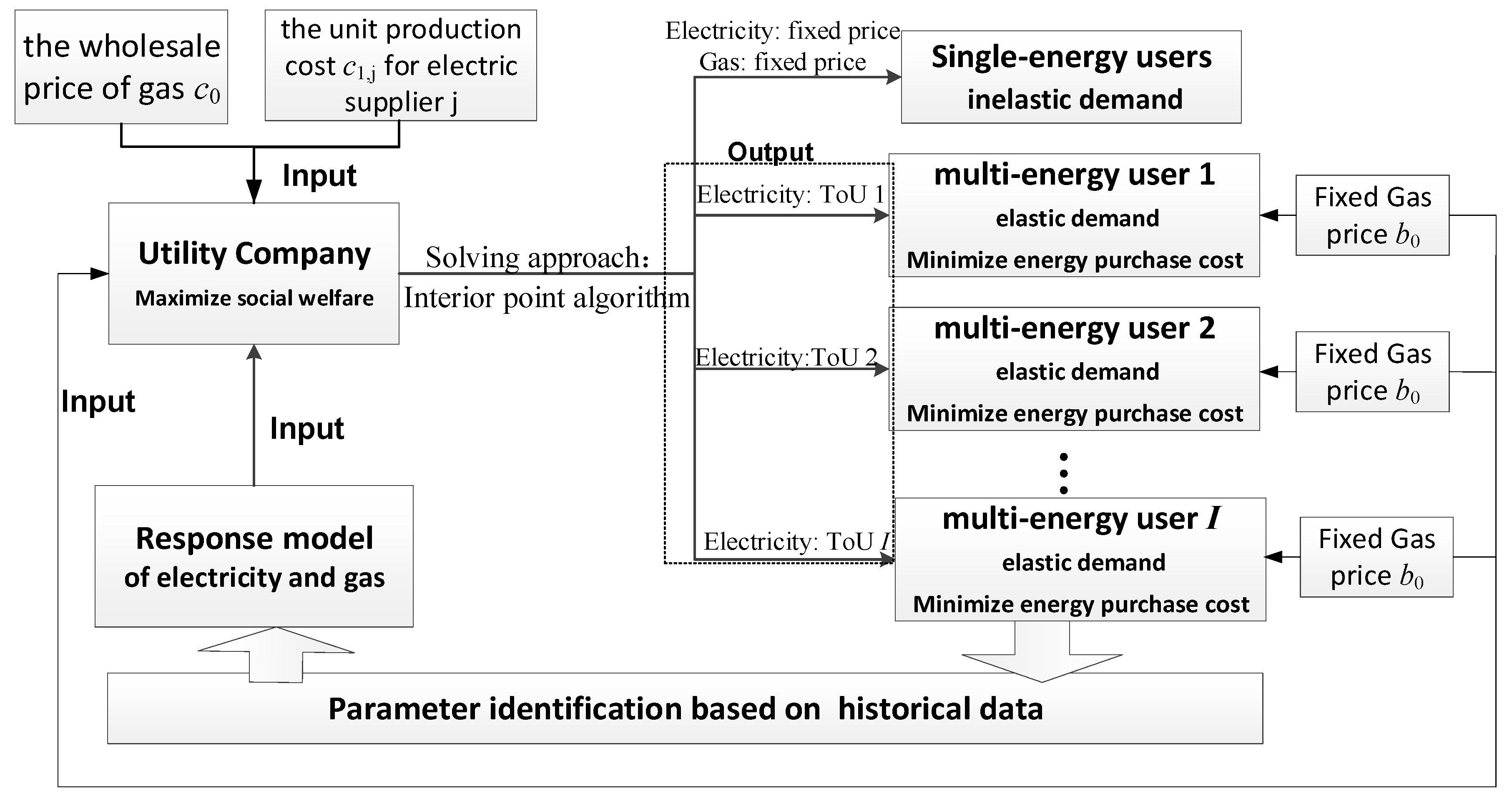
The proposed response model is a result of the consumption behavior of rational customers who choose to adjust the operation of IES to minimize their own energy purchase costs. A utility company, which is a public institution to supply energy such as electricity, gas, or water to the public, is considered as the main character to make energy price in this paper. From the utility company’s point of view, multi-energy DR is expected to maximize the social welfare function 6. In the proposed TOU-based DR scheme, which is illustrated in Figure 4, the goal is achieved by using the TOU electric price signals as a tool to induce multi-energy users to behave in a social-maximizing manner. During the process, the utility company makes various TOU retail price schemes for the multi-energy users at different locations, and the retail gas price for these users is always fixed as the same value. In this section, the problem of determining optimal TOU electric price signals is formulated as an optimization problem with the proposed response model.

According to the response model derived in Section 2, the demands of electricity and gas at the location are functions of electric price vector a = [$a_{\mathrm{p}}^1,a_v^1,a_{\mathrm{f}}^1,\dots ,a_{\mathrm{p}}^I,a_v^I,a_{\mathrm{f}}^I$]^T, where I is the number of buses. It is assumed that gas price is maintaining b₀ at each location. Thus, based on the proposed response model of Equations (18) and (19), the demand functions have the partial derivatives as follows:

$$\frac{\partial x_t^i}{\partial a_t^i}=-\frac{k_1^i}{2b_0}, \frac{\partial x_t^i}{\partial a_f^i}=-\frac{k_0^i}{2b_0}; t\in T_P, T_v$$

(23-1)

$$\frac{\partial x_t^i}{\partial a_f^i}=\frac{-3k_2^i-k_1^i-k_0^i}{2b_0}; t\in T_f$$

(23-2)

$$\frac{\partial y_t^i}{\partial a_t^i}=\frac{k_1^i{a}_t^i+k_0^i{a}_f^i}{2b_0^2}, \frac{\partial y_t^i}{\partial a_f^i}=\frac{k_0^i{a}_t^i+k_2^i{a}_f^i}{2b_0^2}; t\in T_P, T_v$$

(24-1)

$$\frac{\partial y_t^i}{\partial a_f^i}=\frac{\left(k_2^i+2k_0^i+k_1^i\right)a_f^i}{2b_0^2}; t\in T_f$$

(24-2)

where $k_1^i$, $k_2^i$, and $k_0^i$ are the coefficients that depend on the factors of the IES of the multi-energy user at bus i.

Optimization Problem of TOU Pricing

To maximize the social welfare function, the aggregated utility of all users is maximized, and the cost of the overall system is minimized. For multi-energy users, the utility can be regarded as constant due to their certain loads, and the single-energy users are assumed as non-elastic for simplicity, thus leading to a constant utility of the whole system. Hence, for the optimal pricing process for multi-energy users, the objective is to minimize the supply cost of the overall system including the production cost of electricity and gas.

Based on the proposed response model, it is feasible to formulate the problem of determining optimal TOU price signals through a single-level optimization. Consider an energy system comprised of J electricity suppliers and one gas supplier, and their customers are connected to this energy system from I electric buses. The mathematical problem for optimal TOU price can be written as follows.

$$\underset{a,P_{x,}{}_t^i}{min} C(a)={\displaystyle \sum _{t=1}^T\left[{\displaystyle \sum _{i=1}^I{C}_{x,t}^i(P_{x,}{}_t^i)+C_{y,t}^{}(P_{y,t})}\right]}$$

(25)

$$s.t. L_{x,t}\left(P_{x,t},X_t(a)\right)=0; \forall t\in T$$

(26-1)

$$P_{y,t}-{\displaystyle \sum _{i=1}^I{y}_{{}_t}^i(a)=0}; \forall t\in T$$

(26-2)

$$P_{x,t}^{min}\le P_{x,t}\le P_{x,t}^{max}; \forall t\in T$$

(27-1)

$$P_{y,t}^{min}\le P_{y,t}\le P_{y,t}^{max}; \forall t\in T$$

(27-2)

$$a_{}^{min}\le a\le a_{}^{max}; \forall t\in T$$

(27-3)

$$Z_t\left(P_{x,t},x_t(a)\right)\le 0; \forall t\in T$$

(28)

Here, $x_t(a)\triangleq {[x_t^1(a_1),x_t^2(a_2),\dots ,x_t^I(a_I)]}^{\mathrm{T}}$ is the vector of electric demands at different locations, and $y_t^i(a_i)$ is the gas demand at bus i. $P_{x,t}\triangleq {[P_{x,t}^1,P_{x,t}^2,\dots ,P_{x,t}^J]}^{\mathrm{T}}$ is the vector of electricity productions, and P_y,t is the gas wholesale at time slot t. These variables above are decision variables of the optimal pricing problem. In addition, the electric price vector a is also a decision variable. $C_{x,t}^j$ is the electricity production cost at time slot t for supplier j, which is typically modeled with a linear function as follows:

$$C_{x,t}^j(P_{x,t}^{})=c_{1,j}{P}_{x,t}^{}$$

(29)

where c_1,j is the unit production cost for electric supplier j. C_y,t is the gas production cost for the gas supplier,

$$C_{y,t}^{}(P_{y,t}^{})=c_0{P}_{y,t}^{}$$

(30)

where c₀ is the wholesale price of gas. Furthermore, L_x,t is a set of equality constraints about the power balance of the electrical system operation. Formula (26-2) is an equality constraint of the gas balance, which is simplified with the neglect of operation constraints from the gas system. Z_t is a set of inequalities about voltage limits and transmission restrictions of the electrical system. a_min, a_max are the lower and upper limits of the electric price. $P_{x,t}^{min}$, $P_{x,t}^{max}$ are the lower and upper limits of electric generation output, and $P_{y,t}^{min}$, $P_{y,t}^{max}$ are the lower and upper limits of gas production. The decision variables of this problem are based on the partial derivatives in Equations (23) and (24), and the Kuhn–Tucker necessary conditions for the optimization problem are expressed as follows:

$$\frac{d{C}_{x,t}^i}{d{P}_{x,t}^i}=-\frac{\partial L_{x,t}}{\partial P_{x,t}^i}{\Lambda }_t-{\mu }_{x,t}^i-\frac{\partial Z_t}{\partial P_{x,t}^i}{\Pi }_t; \forall t\in T$$

(31)

$$\frac{d{C}_{y,t}^{}}{d{P}_{y,t}^{}}={\Gamma }_t-{\mu }_{y,t}^i; \forall t\in T$$

(32)

$$0=\frac{k_1^i}{2b_0}{\displaystyle \sum _{t=1}^{T_{\sigma }}\frac{\partial L_{x,t}}{\partial x_t^i}}{\Lambda }_t-{\mu }_{x,\sigma }^i+\frac{k_1^i}{2b_0}{\displaystyle \sum _{t=1}^{T_{\sigma }}\frac{\partial Z_t}{\partial x_t^i}}{\Pi }_t; \sigma \in \left\{p,v\right\}$$

(33-1)

$$0=\left(\frac{k_0^i}{2b_0}{\displaystyle \sum _{t=1}^{T_p,T_v}\frac{\partial L_{x,t}}{\partial x_t^i}+}\frac{3k_2^i+k_1^i+k_0^i}{2b_0}{\displaystyle \sum _{t=1}^{T_f}\frac{\partial L_{x,t}}{\partial x_t^i}}\right){\Lambda }_t-{\mu }_{x,f}^i+\left(\frac{k_0^i}{2b_0}{\displaystyle \sum _{t=1}^{T_p,T_v}\frac{\partial Z_t}{\partial x_t^i}}+\frac{3k_2^i+k_1^i+k_0^i}{2b_0}{\displaystyle \sum _{t=1}^{T_f}\frac{\partial Z_t}{\partial x_t^i}}\right){\Pi }_t$$

(33-2)

$$0={\displaystyle \sum _{t=1}^{T_{\sigma }}\frac{k_1^i{a}_t^i+k_0^i{a}_f^i}{2b_0^2}}{\Gamma }_t-{\mu }_{y,\sigma }^i; \sigma \in \left\{p,v\right\}$$

(34-1)

$$0=\left({\displaystyle \sum _{t=1}^{T_p,T_v}\frac{k_2^i{a}_t^i+k_0^i{a}_f^i}{2b_0^2}+{\displaystyle \sum _{t=1}^{T_f}\frac{\left(k_2^i+2k_0^i+k_1^i\right)a_f^i}{2b_0^2}}}\right){\Gamma }_t-{\mu }_{y,f}^i$$

(34-2)

where ${\Lambda }_t$ is the column vector of dual variables corresponding to the equality Constraints (26-1) of electricity systems; ${\Pi }_t$ is the column vector of dual variables corresponding to inequality Constraints (27) of electricity systems; ${\Gamma }_t$ is the column vector of dual variables corresponding to equality Constraints (26-2) of gas balance; ${\mu }_{x,t}^i$, ${\mu }_{y,t}^i$ are dual variables of capacity Constraints (27-1) and (27-2) of electricity and gas, respectively; ${\mu }_{x,\sigma }^i$, ${\mu }_{x,f}^i$, ${\mu }_{y,\sigma }^i$, and ${\mu }_{y,f}^i$ are dual variables corresponding to Constraint (27-3) for electric price limit. The coefficients $k_0^i$, $k_1^i$, $k_2^i$, and gas retail price b₀, gas wholesale price c₀, unit cost of electric production c_1,j are all known parameters.

The optimization problem Equations (25)–(28) can be solved using interior point algorithm, which is highly efficient for a convex problem. The equations, which are constituted with Kuhn–Tucker Conditions (31)–(34), have to be solved in each iteration. The problem finally obtains the optimal solution under the condition that the dual gap converges to 10⁻³. The computation of the time is within 5.9 s on a laptop (ideapad 720S-14IKB, Lenovo, Hong Kong, China) with dual Core-i5 processors clocking at 2.6 GHz and 4 GB of RAM.

4. Case Study

4.1. Analysis of Multi-Energy User’s Response Characteristics

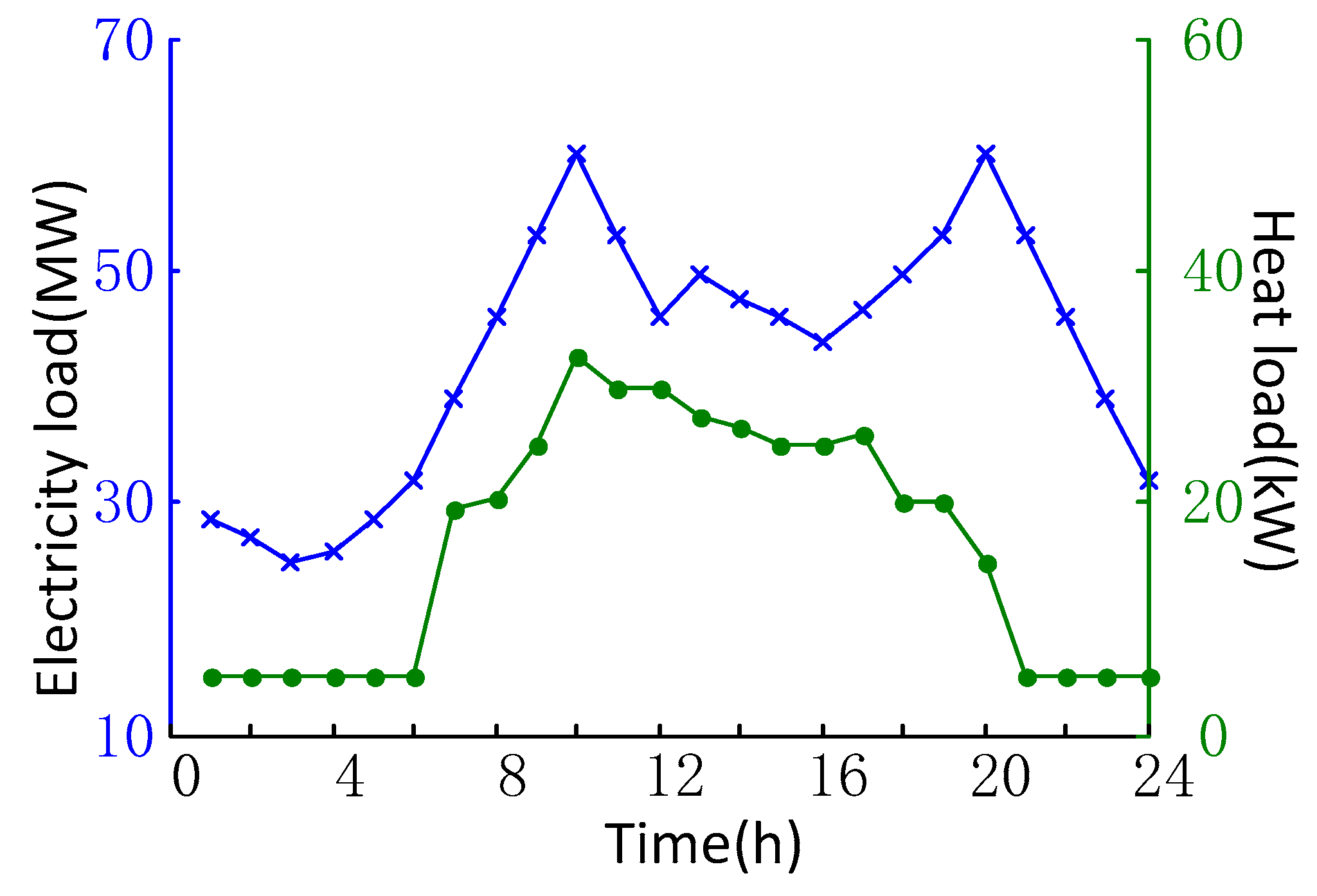
An industrial park with the electric-heat system was adopted to supply both electricity and heat for all users. Here, the industrial park can be seen as a multi-energy user. The capacity of CHP, EB, and TF was 45 MW, 45 MW, and 70 MW, respectively. The coefficients of electric and heat efficiency η_ey, η_hy were both 0.5, m was 200, and n was 0; the conversion efficiency η_ex of TF was 0.97; the heat efficiency η_hx of EB was 0.9. The variations of electricity load and heat load are depicted in Figure 5. The initial electric price of $40/MW and gas price of $90/1000 m³ were assumed as the baseline.

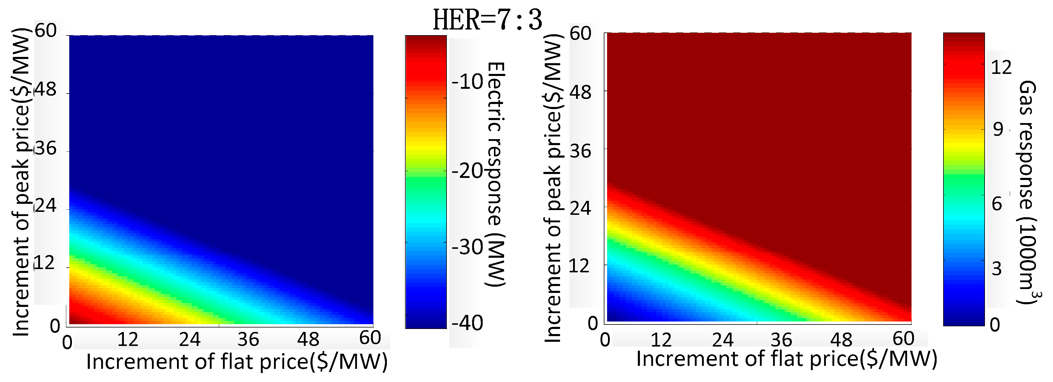
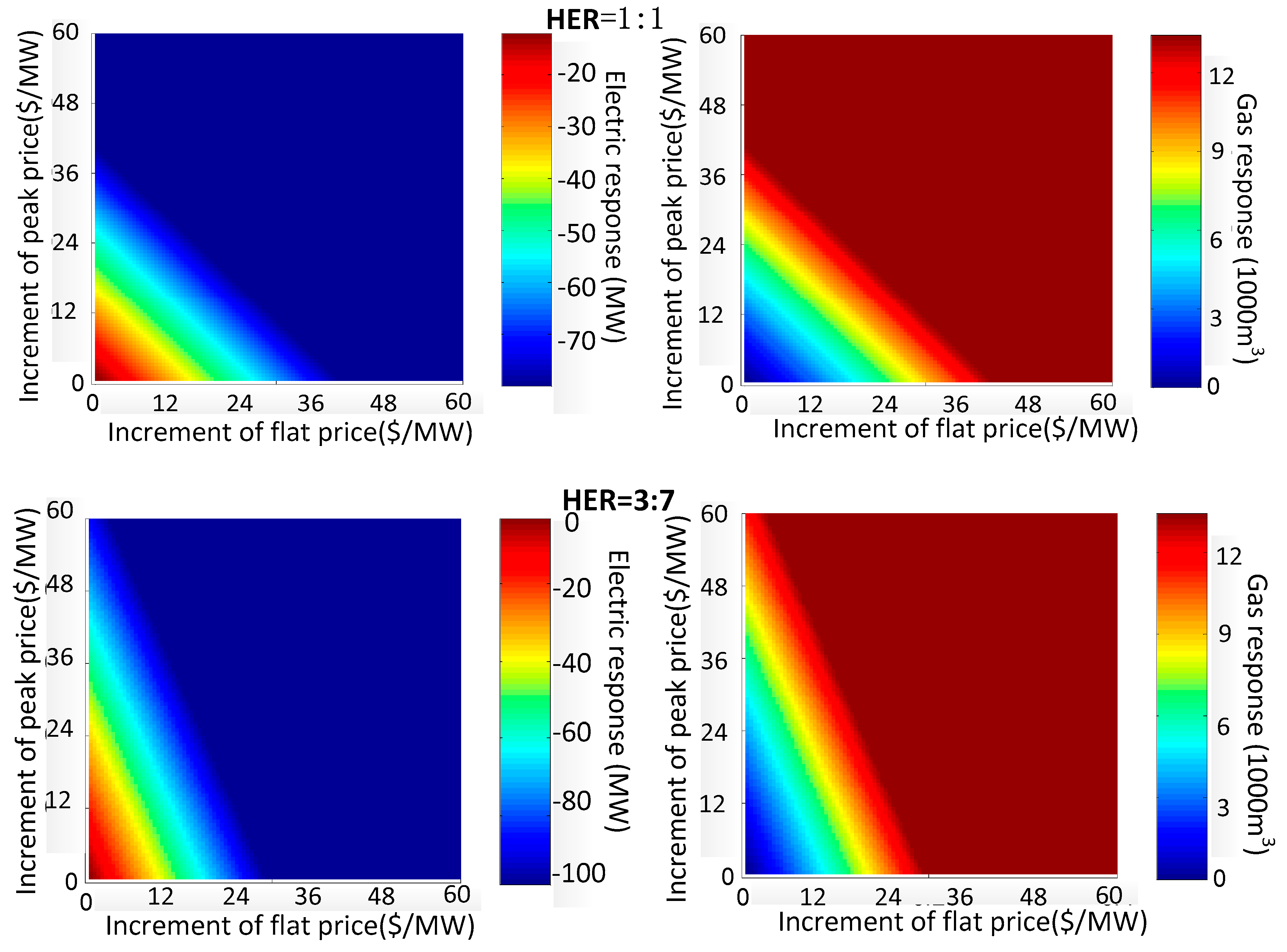
From the response model, the relations between response amount and TOU price depend on the electric and heat efficiency coefficients of IES. Normally, the output heat-to-electricity ratio (HER) of CHP is adjustable to different load conditions. On the condition of keeping the efficiency of other devices constant, the output HER of CHP is varying to formulate the relations of response amount in peak hours and TOU price increment, as illustrated in Figure 6.

The response amount reached a saturated value when electric price rose to some extent due to the restriction of device capacity and the load of IES as aforementioned in Section 2.3. From those chromatograms in Figure 6, the electricity and gas response amount in peak hours were increasing gradually with the rising of peak price and flat price of electricity, and finally, reached a maximum of absolute value. For instance, when HER = 1, the maximum of electric response was −70.8 MW (the minus represents reduced amount), and the maximum of gas response was 13.73 m³.

While HER was 1, the peak–peak elasticity was equal to the peak-flat elasticity (peak-flat elasticity is defined as ${\epsilon }_{pf}=\partial x_p/\partial a_f$); while HER was 7/3, the peak-peak elasticity was larger than the peak-flat elasticity; the contrary was the case while HER was 3/7. Besides, with the HER reduced, the maximum of electricity response in peak hours increased gradually. The reasons are analyzed as follows.

Since the HER of CHP is adjustable, the efficiency coefficients ${\eta }_{hy}$, ${\eta }_{ey}$ are satisfied with Conditions (35).

$${\eta }_{hy}+{\eta }_{ey}=1, 0\le {\eta }_{hy}, {\eta }_{ey}\le 1$$

(35)

Using Formula (16), the electricity response in peak hours is

$$\Delta x_{s,p}=-\left(\frac{{\eta }_{hy}}{{\eta }_{hx}}\frac{{\eta }_{ey}}{{\eta }_{ex}}\Delta a_{s,f}+\frac{{\eta }_{ey}{}^2}{{\eta }_{ex}{}^2}\Delta a_{s,p}\right)\frac{m}{2b_0}=-\left(\frac{\Delta a_{s,p}}{{\eta }_{ex}{}^2}-\frac{\Delta a_{s,f}}{{\eta }_{hx}{\eta }_{ex}}\right){\eta }_{ey}{}^2+\frac{\Delta a_{s,f}}{{\eta }_{hx}{\eta }_{ex}}{\eta }_{ey}$$

(36)

When η_ey = 1, which is corresponding to a minimum HER, it is obvious that Δx_s,p would reach a minimum negative value, which means a maximum response amount. Therefore, a smaller HER would bring about a larger response amount of electricity. Since peak-flat elasticity and peak-peak elasticity are determined by k₀ and k₁, respectively, a smaller HER determines a larger peak-peak elasticity than peak-flat elasticity. Thus, to obtain larger elasticity and response amount from the multi-energy user in the TOU price scheme, the output HER of CHP is better to be smaller.

4.2. Optimal TOU

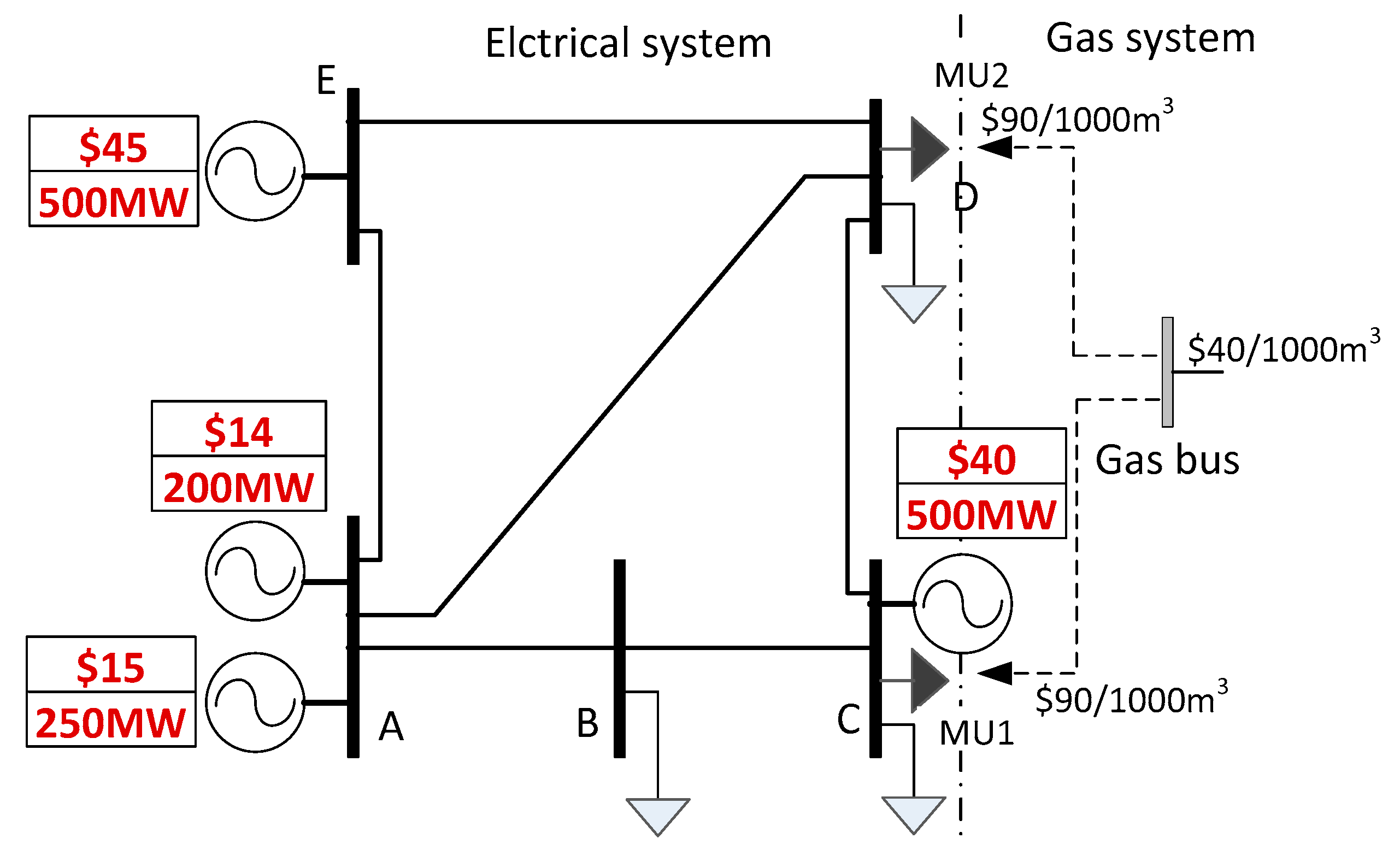
Based on the response model, the TOU pricing strategy was performed on the modified PJM 5-bus system [22]. Two multi-energy users (MU1 and MU2) with the same IES and load conditions were added into the system at buses C and D. The total electric load of other users, which was assumed as non-elastic load, was equally distributed between buses B, C, and D. The modified system is depicted in Figure 7. A utility company is responsible for the electricity and gas supply of the users of this system. The objective of the utility company is to maximize the social welfare as introduced in Section 3. Since the gas grid is omitted in this paper, MU1 and MU2 buy gas from a single gas bus directly at a constant price b₀ ($90/1000 m³ here). The wholesale price c₀ of gas was set as $40/1000 m³ initially. The upper limits of the electric peak, flat, and valley prices were $64/MWh, $40/MWh, and $30/MWh, respectively, and the lower limits were $40/MWh, $30/MWh, and $14/MWh, respectively.

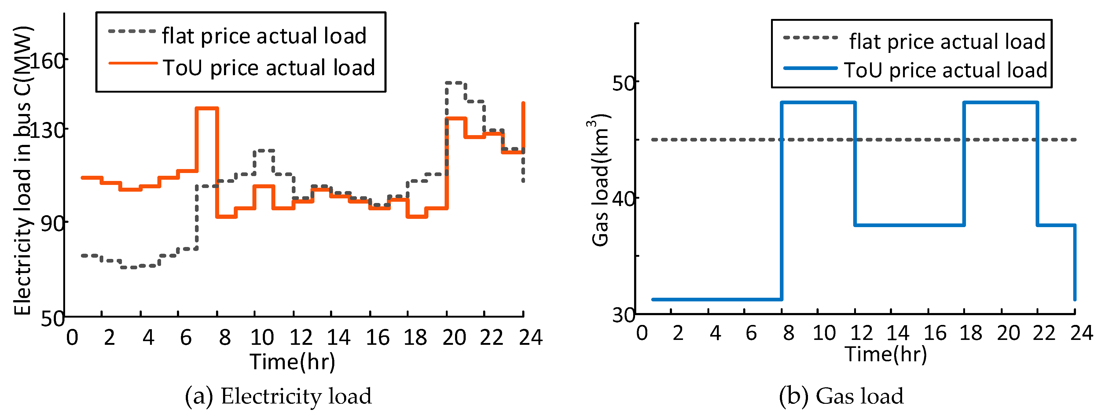
The optimization was performed for a 24-hour interval. The peak hours were defined from 08:00 to 11:00, and 18:00 to 21:00; the valley hours were from 01:00 to 07:00, and 24:00; the rest hours were from 12:00 to 17:00, and 22:00 to 23:00 were flat hours. The proposed TOU scheme was compared with a flat price scheme, in which the electric price for the multi-energy user is constant as $40/MW. The compared results of both electricity load and gas load are depicted in Figure 8.

As expected, the electricity load curve appears gentler in the TOU scheme than the curve in the flat price. The peak load was shed by 16.5% and the valley load increased by 57.1%. Some fluctuations, such as an obvious difference between peak load and valley load, appeared on gas the load curve. Moreover, the total amount of electricity load appeared more than that of the flat price scheme, which is due to the reduced amount of total gas load.

Comparisons of the proposed scheme to the flat-price scheme, in terms of the overall system’s cost and the multi-energy user’s energy purchase cost, are included in

Table 1. Comparing the TOU scheme with flat price scheme.

	Overall System’s Cost ($)	Energy Purchase Cost ($)
Flat price	220,541	125,599
TOU	171,272	107,785

. It can be seen that the TOU scheme reduced 22.34% of the overall system’s cost for the utility company, and meanwhile helped the multi-energy user saves 14.18% of the energy purchase cost, both of which are very desirable for the operation of an integrated energy system.

Since the wholesale price c₀ of gas may fluctuate every few weeks and would affect the TOU pricing of electricity, several levels of wholesale gas price are adopted here to formulate optimal TOU electric prices for the multi-energy users at electric bus C and D.

As presented in

Table 2. The TOU prices of users in bus C and D under various gas production unit cost c₀.

Wholesale Price c0 of Gas ($/1000 m3)	Bus	TOU Electric Price
		Peak	Flat	Valley
20	C	64	40	30
	D	64	40	30
33	C	64	40	30
	D	44.08	40	30
40	C	52.69	33.83	22.20
	D	40	30	14
50	C	40	34.45	23.85
	D	40	30	14
80	C	40	30	14
	D	40	30	14

, when gas wholesale price c₀ belongs to a lower level ($20/1000 m³), the TOU electric price would reach the upper limit of price regardless of whether in peak hours or other hours, for the multi-energy users are expected to consume more gas in a gas-cheaper situation. On the contrary, when gas wholesale price c₀ belongs to a higher level ($80/1000 m³), the TOU electric price would reach the lower limit. For the case where c₀ belongs to a medium level ($33–$50/1000 m³), TOU prices for users in different buses vary a lot. Since electric load at bus C required a higher supply cost than that at bus D, a same gas wholesale price c₀ means higher cost for the user at bus C so that user at bus C is expected to consume more electricity instead of gas. Therefore, with c₀ rising within the medium level, the TOU prices at bus C always appear higher than those at bus D. It depicts that there is a mutual influence between gas market and electricity market. The wholesale price c₀ of gas would affect the retail electric price for multi-energy users if c₀ varies in the range of $20–$80/1000 m³. Beyond this range, the retail TOU price would not vary any more, which means gas wholesale price would have an influence on the electricity retail pricing within a specified range of c₀.

With c₀ at a constant value of $50/1000 m³, several levels of retail gas price b₀ are adopted here to formulate optimal TOU electric prices for the multi-energy users at electric bus C and D. As presented in

Table 3. The TOU prices of users in bus C and D under various gas production unit cost b₀.

Retail Price b0 of Gas ($/1000 m3)	Bus	TOU Electric Price
		Peak	Flat	Valley
50	C	40	30	14
	D	40	30	14
60	C	40	30	30
	D	40	30	16.27
75	C	41.26	33.21	14
	D	40	30	14
90	C	52.69	22.2	33.83
	D	40	30	14
100	C	60	40	30
	D	40	35.28	15.18
115	C	64	40	30
	D	48	40	30
135	C	64	40	30
	D	64	40	30

, when gas retail price b₀ belongs to a lower level ($50/1000 m³), the TOU electric price would still keep as the lower limit. With b₀ rising from $50/1000 m³ to $135/1000 m³, the TOU electric price would increase gradually to the upper limit. It is due to the fact that the response amount is proportional to the electricity-to-gas price ratio from the response model Equations (18) and (19). Thus, in order to obtain a larger response amount, the retail TOU electric price is expected to be increased with retail gas price b₀ rising, to maintain an appropriate electricity-to-gas price ratio. Therefore, it is supposed to ensure an appropriate electricity-to-gas price ratio while considering the electricity and gas’s co-pricing process.

5. Conclusions

Aiming at a better understanding of the response characteristics of multi-energy DR, the energy flow during response process is analyzed, and the multi-energy DR model is proposed based on the derivation of the relations of electricity (gas) response amount and TOU electric price. Then the model is utilized to formulate optimal TOU price, which is one of the typical applications of the response model. Some conclusions have been drawn, as follows:

• The electricity response amount in peak (or valley) hours varies linearly by the increment of electric prices in peak (valley) hours and flat hours; whereas gas response in peak (valley) hours is proportional to the increment of the square of peak (valley) price and flat price.
• The peak–peak elasticity of electricity response is determined by k₁, which depends on the electric efficiency of IES; whereas peak–flat elasticity is determined by k₀, which depends on both electric and heat efficiency.
• A smaller HER of CHP brings about a larger potential of electric response.
• The TOU price scheme is better to smooth electric load curve and, meanwhile, saves more in the overall system’s cost and energy purchase cost than the flat price scheme.
• The decision of TOU electric price should not only compare the marginal cost of electricity supply with wholesale price c₀ of gas, but also ensure an appropriate electricity-to-gas price ratio.

Furthermore, the proposed response model can be modified to adapt to the user with a more complicated energy system.

References

- Moghaddam, I.G.; Saniei, M.; Mashhour, E. A comprehensive model for self-scheduling an energy hub to supply cooling, heating and electrical demands of a building. Energy 2016, 3, 1755–1766. [Google Scholar] [CrossRef]
- Sheikhi, A.; Bahrami, S.; Ranjbar, A.M. An autonomous demand response program for electricity and natural gas networks in smart energy hubs. Energy 2015, 89, 490–499. [Google Scholar] [CrossRef]
- Bahrami, S.; Sheikhi, A. From Demand Response in Smart Grid Toward Integrated Demand Response in Smart Energy Hub. IEEE Trans. Smart Grid 2016, 7, 650–658. [Google Scholar] [CrossRef]
- Kirschen, D.S.; Strbac, G.; Cumperayot, P.; de Paiva Mendes, D. Factoring the elasticity of demand in electricity prices. IEEE Trans. Power Syst. 2000, 15, 612–617. [Google Scholar] [CrossRef]
- Kirschen, D.S. Demand side view of electricity markets. IEEE Trans. Power Syst. 2003, 18, 520–527. [Google Scholar] [CrossRef]
- Yu, R.; Yang, W.; Rahardja, S. A Statistical Demand-Price Model with Its Application in Optimal Real-Time Price. IEEE Trans. Smart Grid 2012, 3, 1734–1742. [Google Scholar] [CrossRef]
- Hayes, B.P.; Melatti, I.; Mancini, T.; Prodanovic, M.; Tronci, E. Residential Demand Management using Individualised Demand Aware Price Policies. IEEE Trans. Smart Grid 2017, 8, 1284–1294. [Google Scholar] [CrossRef]
- Ruan, W.; Wang, B.; Li, Y.; Yang, S. Customer Response Behavior in Time-of-Use Price. Power Syst. Technol. 2014, 36, 86–93. [Google Scholar]
- Houwing, M.; Negenborn, R.R.; Schutter, B.D. Demand response with micro-CHP systems. Proc. IEEE 2011, 99, 200–213. [Google Scholar] [CrossRef]
- Kienzle, F.; Ahcin, P.; Andersson, G. Valuing investments in multi-energy conversion, storage, and demand-side management systems under uncertainty. IEEE Trans. Sustain. Energy 2011, 2, 194–202. [Google Scholar] [CrossRef]
- Papadaska lopoulos, D.; Strbac, G.; Mancarella, P.; Aunedi, M.; Stanojevic, V. Decentralized participation of flexible demand in electricity markets Part II: Application with electric vehicles and heat pump systems. IEEE Trans. Power Syst. 2013, 28, 3658–3666. [Google Scholar] [CrossRef]
- Farshad, J.; Haidar, S.; Reza, S.A.; Rastegar, M. Developing a two-step method to implement residential demand response programmes in multi-carrier energy systems. IET Gener. Transm. Distrib. 2018, 12, 2614–2623. [Google Scholar]
- Shi, Q.; Li, F.; Hu, Q.; Wang, Z. Dynamic demand control for system frequency regulation: Concept review, algorithm comparison, and future vision. Electr. Power Syst. Res. 2018, 154, 75–87. [Google Scholar] [CrossRef]
- Galus, M.D.; Koch, S.; Andersson, G. Provision of load frequency control by PHEVS, controllable loads, and a cogeneration unit. IEEE Trans. Ind. Electron. 2011, 58, 4568–4582. [Google Scholar] [CrossRef]
- Csetvei, Z.; Østergaard, J.; Nyeng, P. Controlling price-responsive heat pumps for overload elimination in distribution systems. In Proceedings of the 2nd IEEE PES International Conference and Exhibition on Innovative Smart Grid Technologies, Manchester, UK, 5–7 December 2011. [Google Scholar]
- Wang, D.; Parkinson, S.; Miao, W.; Jia, H.; Crawford, C.; Djilali, N. Online voltage security assessment considering comfort-constrained demand response control of distributed heat pump systems. Appl. Energy 2012, 96, 104–114. [Google Scholar] [CrossRef]
- Mancarella, P.; Chicco, G. Real-Time Demand Response from Energy Shifting in Distributed Multi-Generation. IEEE Trans. Smart Grid 2013, 4, 1928–1938. [Google Scholar] [CrossRef]
- Shao, C.; Ding, Y.; Siano, P.; Lin, Z. A Framework for Incorporating Demand Response of Smart Buildings into the Integrated Heat and Electricity Energy System. IEEE Trans. Ind. Electron. 2019, 66, 1465–1475. [Google Scholar] [CrossRef]
- Geidl, M.; Koeppel, G.; Favre-Perrod, P.; Klockl, B.; Andersson, G.; Frohlich, K. Energy hubs for the future. Power Energy Mag. IEEE 2007, 5, 24–30. [Google Scholar] [CrossRef]
- Sheikhi, A.; Rayati, M.; Bahrami, S.; Ranjbar, A.M. Demand side management in a group of Smart Energy Hubs as price anticipators; the game theoretical approach. In Proceedings of the 2015 IEEE Power & Energy Society Innovative Smart Grid Technologies Conference (ISGT), Washington, DC, USA, 18–20 February 2015. [Google Scholar]
- Chicco, G.; Mancarella, P. Matrix modelling of small-scale trigeneration systems and application to operational optimization. Energy 2009, 34, 261–273. [Google Scholar] [CrossRef]
- PJM Training Materials—LMP101. Available online: http://www.pjm.com/training/training-material.aspx (accessed on 31 July 2017).
Figure 1.
The schematic diagram of an electric-heat system.
Figure 2.
Multi-energy user’s options of meeting electricity and heat load.
Figure 3.
The energy flow in the multi-energy system.
Figure 4.
The proposed time-of-use (TOU) scheme.
Figure 5.
Profiles of electricity and heat load of multi-energy user.
Figure 6.
Relations between electric (gas) response in peak hours and increment of the peak, flat price under various heat-to-electricity ratios (HERs).
Figure 7.
An energy system with two multi-energy users.
Figure 8.
Comparison of the actual load curve at electric bus C under the TOU scheme and the flat-price scheme.