Short-Term Load Forecasting with Tensor Partial Least Squares-Neural Network

Abstract

Short-term load forecasting is very important for power systems. The load is related to many factors which compose tensors. However, tensors cannot be input directly into most traditional forecasting models. This paper proposes a tensor partial least squares-neural network model (TPN) to forecast the power load. The model contains a tensor decomposition outer model and a nonlinear inner model. The outer model extracts common latent variables of tensor input and vector output and makes the residuals less than the threshold by iteration. The inner model determines the relationship between the latent variable matrix and the output by using a neural network. This model structure can preserve the information of tensors and the nonlinear features of the system. Three classical models, partial least squares (PLS), least squares support vector machine (LSSVM) and neural network (NN), are selected to compare the forecasting results. The results show that the proposed model is efficient for short-term load and daily load peak forecasting. Compared to PLS, LSSVM and NN, the TPN has the best forecasting accuracy.

1. Introduction

Load forecasting is very important in the planning, operation and maintenance of power system [1,2]. The short-term forecasting technique can be used to predict the load in the next few hours or days. The forecasting accuracy directly affects the generation plan, the optimal combination of the generator, power flow calculation, electricity market transaction, power real-time dispatching, etc.

A good prediction model is always the key issue of load forecasting. Traditionally, forecasting was mainly based on the previous information of a certain time period of the load situation. In spite of the length of the time period, from the perspective of the data structure, the input of the prediction model is a time series of the power load. In fact, besides the previous situation, the power load is also related to many factors such as seasons, meteorological conditions and people’s living habits [3,4]. In order to improve the forecasting accuracy of load, the influence of these factors must be considered. Therefore, the input of the prediction model changes from time series to tensor, which has a complex structure [5]. Tensors are physical quantities which can be expressed by combinations of several base vectors and their components. Theoretically, tensors can represent physical quantities with arbitrary complex relations since the abundant combinations of base vectors. Using tensors to express the multiple factors affecting power load accords with the essential characteristics of the factors. Because the factors have different measurement and characterization methods, it may cause information loss if the data obtained from these factors were represented in the same dimension. Although the information and relationships in different dimensions represented by tensors are recessive, the representation method retains the complete information of the high-dimensional data and the recessive relationships can be explicated by tensor algorithms.

Some regression algorithms are adopted for building prediction models. Partial least squares (PLS) is a classical model which maps the variables in a new feature space with lower dimensions. It is widely used in various fields such as fault detection and diagnosis, robot, industrial process control, traffic safety, etc. [6,7,8,9]. However, The method cannot be used directly for tensors. Some improved methods, which are combined with unfolding, are proposed [10,11]. The main idea of unfolding is converting tensors into matrices so that original tensors can be replaced by the matrices which reserve the original values of every element. This process destroys the structure of tensors which may include a priori information and makes the physical meaning of data hard to understand [5,12]. The higher-order PLS (HOPLS) technique projects tensors into latent space and applied PLS regression for corresponding latent variables [13]. The method cannot be used when the output of the model is a one-dimensional tensor, namely vector. N-way PLS decomposes independent and dependent data into rank-one tensors [14,15]. The decomposition must be subject to maximum pairwise covariance of the latent vectors. Canonical decomposition for tensors affects the computational complexity, the convergence speed and the fitness ability directly [16]. Furthermore, both HOPLS and N-way PLS focus on the linear correlations between inputs and outputs of the models. Nonlinear characteristics of the data will reduce the forecasting accuracy. Neural network (NN), which is a classical nonlinear regression algorithm, learns knowledge and determines parameters from the samples without mathematical derivations. Many adaptive forecast and control methods based on NN are proposed to research and analyze nonlinear uncertain systems. For example, there are results including multiagent [17,18], full state constraints [19,20], uncertain nonlinear stochastic systems [21] and nonlinear MIMO systems [22]. However, computational efforts of NN are substantial with the increasing complexity of the network structure. In addition, black-box structures make knowledge hard to understand [23]. Least squares support vector machine (LSSVM) is another common nonlinear regression algorithm which is improved based on the support vector machine (SVM). The core idea is to map low-dimensional nonlinear problems to linear problems in high-dimensions. LSSVM performs competently on some issues [24,25,26], but it may lose the sparseness of support vectors [27]. Moreover, for forecasting with tensor input, a tensors-to-matrices simplification process is needed for NN and LSSVM methods, during which it is bound to lose some potentially useful information.

In this paper, a tensor partial least squares-neural network (TPN) method is proposed for load forecasting. The method integrates an outer model and an inner model. The outer model is used to decomposition the input tensors. Tensor PLS decomposition is used in it since the method can extract common latent variables of the input and output of the system. However, PLS is a linear method. It can be used for tensor decomposition but it is not suitable for nonlinear predictive modeling. Therefore, the inner model, which is used to forecast, needs a nonlinear structure. Since NN can approximate any nonlinear function at a sufficient accuracy, it is selected to set up the inner model. According to the structure of the prediction model, the input and output of the system are projected into a low-dimensional common latent subspace in the outer model and latent variables extracted by the outer model are used as the input of the inner model. The modeling process involves linear decomposition, non-linear fitting and spatial mapping. So, three classical models (PLS, NN and LSSVM), which are typical representatives of the ideas above, are used to measure the forecast results.

2. Proposed Method

For the TPN, data from p measuring time points form the input tensor and can be represented by

$$\underset{\_}{\mathbf{X}}={({\mathbf{X}}_{\lambda 1},{\mathbf{X}}_{\lambda 2},\cdots ,{\mathbf{X}}_{\lambda p})}_{I_1\times I_2\times I_3}$$

(1)

where ${\mathbf{X}}_{\lambda 1},i\in \{1,\cdots p\}$ is the data obtained from the ith measuring time point. I₁ is the number of samples. I₂ is the number of measuring times. I₃ is the number of parameters.

$\mathbf{y}={(y_1,y_2,\cdots y_n)}_{I_1\times 1}^T$ represents the loads of the power system and it is the output vector. TPN contains a linear outer model and a nonlinear inner model. The outer model is built by tensor partial least squares and the inner model is built by the neural network. The structure of TPN is shown in Figure 1.

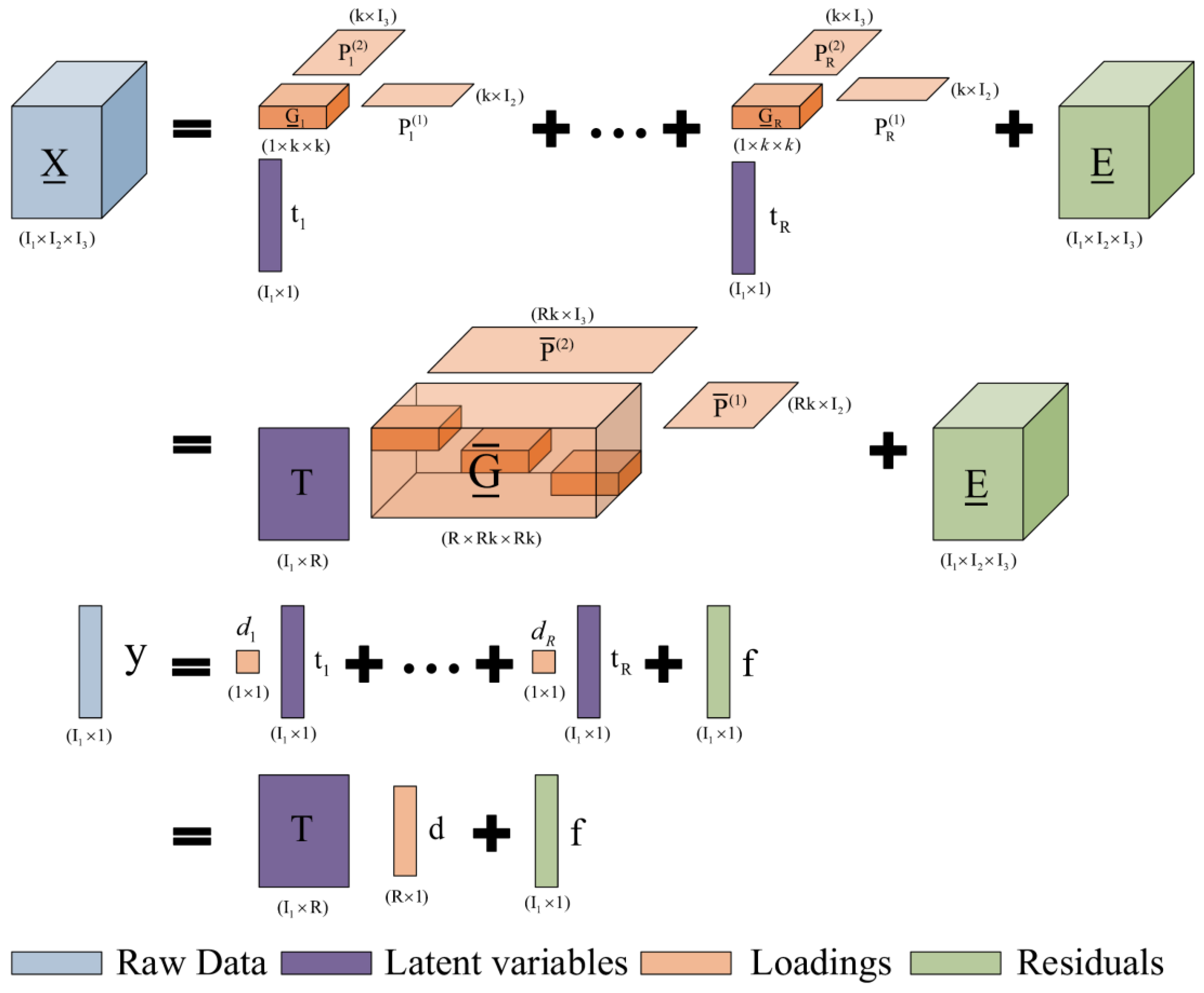
X and y are projected into a subspace which has common latents. The parameters can be determined by the decomposition process. Because X and y have the same number of samples, X can be represented as

$$\begin{array}{ll}\underset{\_}{\mathbf{X}}& ={\displaystyle \sum _{r=1}^R{\underset{\_}{\mathbf{G}}}_r{\times }_1{\mathbf{t}}_r{\times }_2{\mathbf{P}}_r^{(1)}{\times }_3{\mathbf{P}}_r^{(2)}}+{\underset{\_}{\mathbf{E}}}_R\\ & =\overline{\underset{\_}{\mathbf{G}}}{\times }_1\mathbf{T}{\times }_2{\overline{\mathbf{P}}}^{(1)}{\times }_3{\overline{\mathbf{P}}}^{(2)}+{\underset{\_}{\mathbf{E}}}_R\end{array}$$

(2)

where ${\underset{\_}{\mathbf{G}}}_r$ is the rth rank-(1, k, k) tensor. ${\mathbf{t}}_r$ is the rth latent variable. r is the iteration times. R is the number of latent variables. ${\mathbf{P}}^{(1)}$ and ${\mathbf{P}}^{(2)}$ are the first and the second loading matrices. The operation ×_n denotes the n-mode product [13]. $\overline{\underset{\_}{\mathbf{G}}}$ is the core tensor which has a special block-diagonal structure and the elements indicate the level of local interactions between the loading matrices and the corresponding latent vectors. T is the latent variable matrix and t_r is the rth column of T. ${\mathbf{P}}_r^{(1)}$ and ${\mathbf{P}}_r^{(2)}$ can be gotten by singular value decomposition (SVD) [28,29,30].

y could be represented as

$$\mathbf{y}=\mathbf{Td}+\mathbf{f}$$

(3)

where d is the loading vector. f is the residual of y. The schematic diagram of the decomposition procedure is shown in Figure 2.

Then NN is used to build the inner model. Equation (3) can be represented as

$$\mathbf{y}=s(\mathbf{T})+\mathbf{f}$$

(4)

where s(T) is the output of the NN model.

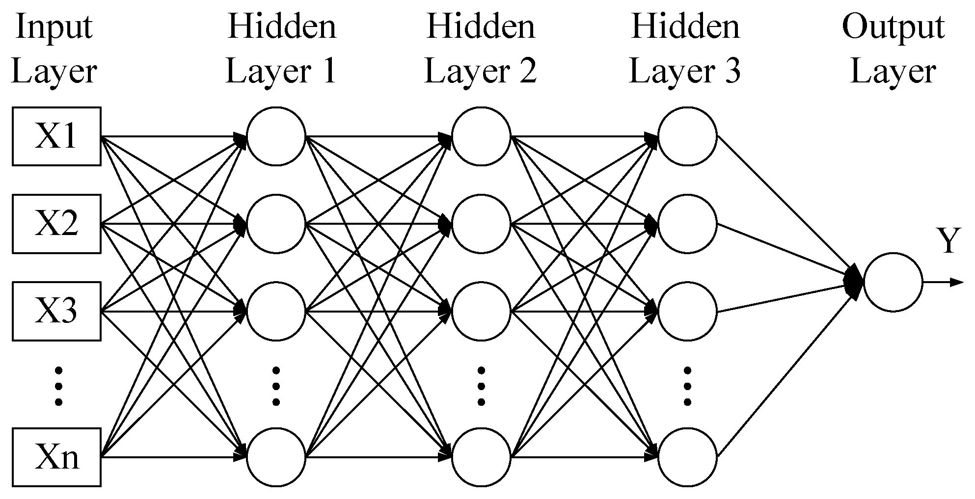
Generally, NN has an input layer, an output layer and several hidden layers. A neuron is an activation function containing weight and bias parameters. The number of neurons in the hidden layer is usually determined by expert knowledge. For TPN in this paper, the number is 3. Figure 3 shows the structure of NN with three hidden layers. The inner model uses a back-propagation neural network (BPNN) to iterate. The learning procedure includes the feed-forward stage and the error back-propagation stage. In the feed-forward stage, the sigmoid function, the weights and the values at the previous layer are used to calculate the values. In the error back-propagation stage, the weights are modified by feedback. The two stages are repeated until the output values converge to the target values.

For a new input sensor ${\underset{\_}{\mathbf{X}}}^{\prime }$, the forecast value ${\widehat{\mathbf{y}}}^{\prime }$ can be expressed as

$${\widehat{\mathbf{y}}}^{\prime }=s({\mathbf{T}}^{\prime })+\mathbf{f}\approx s({\mathbf{T}}^{\prime })$$

(5)

f can be ignored if it is less than the threshold value by iteration.

3. Brief Introduction of Comparative Models

3.1. PLS

The relationship between input and output of PLS model can be written as

$$\mathbf{y}=\mathbf{X}\beta +\epsilon$$

(6)

where X is the input matrix. y is the output vector. β is a matrix of regression coefficients. ε is a bias vector.

It supposes that a small number of principal components are defined by linear combinations of the input matrix. The original linear relationship can be rewritten as

$$\mathbf{y}=\mathbf{T}v+\epsilon$$

(7)

where v is a vector of regression coefficients corresponding to the latent variables. T is a matrix and it can be estimated as

$$\mathbf{T}=\mathbf{X}\mathbf{W}{({\mathbf{P}}^T\mathbf{W})}^{-1}$$

(8)

where P is the loading matrix representing the influence of X. W is the weight loading matrix indicating the correlation between output and input.

3.2. LSSVM

In the LSSVM model, a linear estimation is performed between the input X and the output y

$$\mathbf{y}=\omega \mathbf{X}+b$$

(9)

where ω is a weight coefficients matrix. b is a threshold vector.

It supposes that ω can be written by a Lagrange multiplier as follows:

$$\omega ={\displaystyle \sum _{i=1}^N{\alpha }_i{x}_i}$$

(10)

where x_i is a variable of input matrix X. α_i is the Lagrange coefficient corresponding to x_i.

Then Equation (9) can be written as

$$\mathbf{y}={\displaystyle \sum _{i=1}^N{\alpha }_i{x}_i{}^T\mathbf{X}+b={\displaystyle \sum _{i=1}^N{\alpha }_i\langle x_i{}^T,\mathbf{X}\rangle +b}}$$

(11)

where $\langle x_i{}^T,\mathbf{X}\rangle$ is the inner product. It can be replaced by a kernel function K(x_i, X) and the nonlinear equation can be established by

$$\mathbf{y}={\displaystyle \sum _{i=1}^N{\alpha }_{i}K(x_i,\mathbf{X})+b}$$

(12)

3.3. NN

Similarly, BPNN is chosen for comparison. The schematic diagram of the NN structure is similar to the inner model of TPN, as shown in Figure 3. The activation function is a Sigmoid-type function. The number of hidden layers is 3.

4. Forecast Results and Discussion

4.1. Data Interpretation

The power system load is related to many factors. Besides the known prior load data, the environment temperature and lifestyle (working or rest days), which are two major factors of load, are used to build the prediction models [31]. The data set is a part ofthe 2014 Global Energy Forecasting Competition Load Forecasting (GEFCOM2014-L) which contains load data from 1 January 2010 to 31 December 2014. The original data is a time series. For each time point, the element contains three dimensions, which are load, temperature and date. In the summer, the correlation between temperature and load is the highest [32]. So the summer (June, July and August) load data is used. The set contains 11,040 actual datums. The temperature information comes from weather stations and the load information comes from power grid companies. The sampling time interval is one hour. The data are divided into the calibration set (90% of the data) and test set (10% of the data). The calibration set is used to train and determine the coefficients of the prediction model. The test set is used to evaluate effectiveness. For TPN, set p = 24 in Equation (1). This means that the input of the system is 24-h continuous data. So I₁ = 11040/24 × 90% = 414 (the number of samples), I₂ = 1 (the number of measuring time) and I₃ = 3 (the number of parameters). For PLS, LSSVM and NN, since the input of these models must be a matrix, the tensor input needs the slicing processing. Load matrix, temperature matrix and date matrix are combined into a large input matrix. The matrix contains 414 rows and 72 columns (there are 24 columns of load data, temperature data and date data, respectively). Root mean square error (RMSE) and mean absolute percentage error (MAPE) are used to evaluate the forecasting accuracies of the models. The two evaluation indexes can be calculated by

$$\mathrm{RMSE}=\sqrt{\frac{1}{\mathrm{n}}{\displaystyle \sum _{i=1}^n({\widehat{y}}_n-}{y}_n{)}^2}$$

(13)

$$\mathrm{MAPE}=\frac{1}{n}{\displaystyle \sum _{i=1}^n\frac{\left|{\widehat{y}}_n-y_n\right|}{y_n}}\times 100\%$$

(14)

where $y_n$ is the actual load of the test set. ${\widehat{y}}_n$ is the predicted load. n is the size of the test set.

4.2. Load Forecasting

Hourly loads in the next 12 h are forecasted.

Table 1. The root mean square error (RMSE) of four prediction models.

	Model	PLS	LSSVM	NN	TPN
Hour
1		60.60	101.00	58.74	42.55
2		60.80	99.00	76.57	42.61
3		61.29	96.42	75.84	43.21
4		62.27	94.80	97.88	44.94
5		72.05	100.42	145.19	53.20
6		103.49	135.77	126.02	78.61
7		150.29	201.60	175.71	121.09
8		175.88	226.68	182.10	146.10
9		172.24	210.88	226.69	142.99
10		186.62	207.55	246.46	141.62
11		199.03	220.66	190.12	150.84
12		211.25	236.84	206.86	158.24

and

Table 2. The mean absolute percentage error (MAPE) of four prediction models.

	Model	PLS	LSSVM	NN	TPN
Hour
1		1.53%	2.53%	1.56%	1.07%
2		1.53%	2.48%	1.91%	1.07%
3		1.54%	2.41%	1.89%	1.08%
4		1.55%	2.40%	2.54%	1.12%
5		1.82%	2.51%	3.42%	1.36%
6		2.59%	3.38%	3.65%	1.96%
7		3.73%	5.04%	4.39%	3.02%
8		4.40%	5.30%	4.56%	3.64%
9		4.45%	5.29%	5.67%	3.67%
10		4.67%	5.38%	6.16%	3.54%
11		5.07%	5.61%	5.75%	3.79%
12		5.33%	5.92%	5.17%	3.95%

show the RMSE and MAPE of the proposed model and three comparative models, respectively. Figure 4 shows the trends of RMSE and MAPE. In each forecasting, both the RMSE and MAPE of the proposed model are the lowest. This indicates that the forecasting ability of TPN is the highest. The main reason is that the TPN outer model preserves the features and information of the input tensors and the inner model uses nonlinear structure. When the predicted interval is longer than 6 h, the forecasting accuracies of all four models are obviously reduced. This indicates that the correlation between temperature and load decreases with the predicted interval increasing, as well as lifestyle.

4.3. Daily Load Peak Forecasting

TPN can also forecast the daily load peak and peak appearance time.

Table 3. The forecasting result of daily load peak and peak appearance time.

Output	PLS	LSSVM	NN	TPN
peak	231.44	251.70	293.71	167.56
time	2.36	2.47	2.60	2.48

shows the forecasting result. Compared with the other three models, TPN has the highest daily load peak forecasting ability. There is little difference between the forecasting results of the four models for peak appearance time and the results are unsatisfactory. The main reason is that the actual peak appearance time is a timescale, but the outputs of the models are scalar quantities.

4.4. Discussion of the Results

Power load is affected by many factors. These factors constitute different dimensions of the system input. The relationship between different dimensions classifies as important information of the system. Usually, the information which is related to predict output is invisible. Restricted by the dimension of input data, traditional forecasting models such as PLS, LSSVM and NN need to reduce the dimensions of input. This process may cause the loss of hidden information. Using tensors to represent the system input can avoid this problem. In theory, tensors can accurately describe the invisible relationship between data in different dimensions without information loss. For TPN, the outer model, which used tensor PLS, can preserve the high dimensional structure of tensors. The inner model, which used NN, is very suitable for processing invisible information. This hidden information improves the prediction accuracy of the TPN model.

5. Conclusions

This paper proposed a short-term load forecasting model with the tensor partial least squares-neural network. The model regards prior load data and other relevant quantities (temperatureand lifestyle) as multisense tensors. The data processing method, which combines the outer model and inner nonlinear model, can avoid information loss to a certain extent. Compared with classical PLS, LSSVM and NN, the proposed model has the highest forecasting accuracy.

References

- Hu, R.; Wen, S.; Zeng, Z.; Huang, T. A short-term power load forecasting model based on the generalized regression neural network with decreasing step fruit fly optimization algorithm. Neurocomputing 2017, 221, 24–31. [Google Scholar] [CrossRef]
- Quan, H.; Srinivasan, D.; Khosravi, A. Short-term load and wind power forecasting using neural network-based prediction intervals. IEEE Trans.Neural Netw. Learn. 2014, 25, 303–315. [Google Scholar] [CrossRef] [PubMed]
- Monteiro, C.; Ramirez-Rosado, I.J.; Fernandez-Jimenez, L.A.; Ribeiro, M. New probabilistic price forecasting models: Application to the Iberian electricity market. Int. J. Electr. Power Energy Syst. 2018, 103, 483–496. [Google Scholar] [CrossRef]
- van der Meer, D.W.; Munkhammar, J.; Widen, J. Probabilistic forecasting of solar power, electricity consumption and net load: Investigating the effect of seasons, aggregation and penetration on prediction intervals. Sol. Energy 2018, 171, 397–413. [Google Scholar] [CrossRef]
- Kolda, T.G.; Bader, B.W. Tensor decompositions and applications. SIAM Rev. 2009, 51, 455–500. [Google Scholar] [CrossRef]
- Li, Q.M.; Yan, Y.; Wang, H.Z. Discriminative weighted sparse partial least squares for human detection. IEEE Trans. Intell. Trans. Syst. 2016, 17, 1062–1071. [Google Scholar] [CrossRef]
- Zhong, B.; Wang, J.; Zhou, J.; Wu, H.; Jin, Q. Quality-related statistical process monitoring method based on global and local partial least-squares projection. Ind. Eng. Chem. Res. 2016, 55, 1609–1622. [Google Scholar] [CrossRef]
- Hattori, Y.; Otsuka, M. Modeling of feed-forward control using the partial least squares regression method in the tablet compression process. Int. J. Pharm. 2017, 524, 407–413. [Google Scholar] [CrossRef]
- Yi, J.; Huang, D.; He, H.B.; Zhou, W.; Han, Q.; Li, T.F. A novel framework for fault diagnosis using kernel partial least squares based on an optimal preference matrix. IEEE Trans. Ind. Electron. 2017, 64, 4315–4324. [Google Scholar] [CrossRef]
- Letexier, D.; Bourennane, S.; Talon, J.B. Nonorthogonal tensor matricization for hyperspectral image filtering. IEEE Geosci. Remote Sens. Lett. 2008, 5, 3–7. [Google Scholar] [CrossRef]
- Zhou, G.X.; Zhao, Q.B.; Zhang, Y.; Adali, T.; Xie, S.L.; Cichocki, A. Linked component analysis from matrices to high-order tensors: Applications to biomedical data. Proc. IEEE 2016, 104, 310–331. [Google Scholar] [CrossRef]
- De Lathauwer, L. Decompositions of a higher-order tensor in block terms-part II: Definitions and uniqueness. SIAM J. Matrix Anal. Appl. 2008, 30, 1033–1066. [Google Scholar] [CrossRef]
- Zhao, Q.B.; Caiafa, C.F.; Mandic, D.P.; Chao, Z.C.; Nagasaka, Y.; Fujii, N.; Zhang, L.Q.; Cichocki, A. Higher order partial least squares (HOPLS): A generalized multilinear regression method. IEEE Trans. Pattern Anal. Mach. Intell. 2013, 35, 1660–1673. [Google Scholar] [CrossRef]
- Eliseyev, A.; Auboiroux, V.; Costecalde, T.; Langar, L.; Charvet, G.; Mestais, C.; Aksenova, T.; Benabid, A.L. Recursive exponentially weighted N-way partial least squares regression with recursive-validation of hyper-parameters in brain-computer interface applications. Sci. Rep. 2017, 7, 16281. [Google Scholar] [CrossRef]
- Hervas, D.; Prats-Montalban, J.M.; Lahoz, A.; Ferrer, A. Sparse N-way partial least squares with R package sNPLS. Chemom. Intell. Lab. Syst. 2018, 179, 54–63. [Google Scholar] [CrossRef]
- Cao, H.; Yan, X.; Yang, S.; Ren, H.; Ge, S.S. Low-cost pyrometry system with nonlinear multisense partial least squares. IEEE Trans. Syst. Man Cybern. Syst. 2018, 48, 1029–1038. [Google Scholar] [CrossRef]
- Wen, G.; Chen, C.L.P.; Liu, Y.J.; Liu, Z. Neural network-based adaptive leader-following consensus control for a class of nonlinear multiagent state-delay systems. IEEE Trans. Cybern. 2017, 47, 2151–2160. [Google Scholar] [CrossRef]
- Hua, C.; Zhang, L.; Guan, X. Distributed adaptive neural network output tracking of leader-following high-order stochastic nonlinear multiagent systems with unknown dead-zone input. IEEE Trans. Cybern. 2017, 47, 177–185. [Google Scholar] [CrossRef]
- He, W.; Chen, Y.; Yin, Z. Adaptive neural network control of an uncertain robot with full-state constraints. IEEE Trans. Cybern. 2016, 46, 620–629. [Google Scholar] [CrossRef]
- Liu, Y.J.; Li, J.; Tong, S.; Chen, C.L.P. Neural network control-based adaptive learning design for nonlinear systems with full-state constraints. IEEE Trans. Neural Netw. Learn. 2016, 27, 1562–1571. [Google Scholar] [CrossRef]
- Chen, C.L.P.; Liu, Y.J.; Wen, G.X. Fuzzy neural network-based adaptive control for a class of uncertain nonlinear stochastic systems. IEEE Trans. Cybern. 2014, 44, 583–593. [Google Scholar] [CrossRef]
- Hwang, C.L.; Hung, J.Y. Adaptive recurrent neural network enhanced variable structure control for nonlinear discrete MIMO systems. Asian J. Control 2018, 20, 2101–2115. [Google Scholar] [CrossRef]
- Liu, D.; Wang, D.; Zhao, D.; Wei, Q.; Jin, N. Neural-network-based optimal control for a class of unknown discrete-time nonlinear systems using globalized dual heuristic programming. IEEE Trans. Autom. Sci. Eng. 2012, 9, 628–634. [Google Scholar] [CrossRef]
- Hoang, N.D.; Bui, D.T. Predicting earthquake-induced soil liquefaction based on a hybridization of kernel fisher discriminant analysis and a least squares support vector machine: a multi-dataset study. Bull. Eng. Geol. Environ. 2018, 77, 191–204. [Google Scholar] [CrossRef]
- Wu, Y.H.; Shen, H. Grey-related least squares support vector machine optimization model and its application in predicting natural gas consumption demand. J. Comput. Appl. Math. 2018, 338, 212–220. [Google Scholar] [CrossRef]
- Liu, C.; Tang, L.X.; Liu, J.Y. Least squares support vector machine with self-organizing multiple kernel learning and sparsity. Neurocomputing 2019, 331, 493–504. [Google Scholar] [CrossRef]
- Cheng, Q.; Tezcan, J.; Cheng, J. Confidence and prediction intervals for semiparametric mixed-effect least squares support vector machine. Pattern Recogn. Lett. 2014, 40, 88–95. [Google Scholar] [CrossRef]
- Taubenschuss, U.; Santolik, O. Wave polarization analyzed by singular value decomposition of the spectral matrix in the presence of noise. Surv. Geophys. 2019, 40, 39–69. [Google Scholar] [CrossRef]
- Li, H.; Liu, T.; Wu, X.; Chen, Q. Research on bearing fault feature extraction based on singular value decomposition and optimized frequency band entropy. Mech. Syst. Signal Process. 2019, 118, 477–502. [Google Scholar] [CrossRef]
- Pitton, G.; Heltai, L. Accelerating the iterative solution of convection-diffusion problems using singular value decomposition. Numer. Linear Algebra Appl. 2018, 26, e2211. [Google Scholar] [CrossRef]
- Zhong, J.; Zhao, B.; Zhang, D.; Bao, H. Quantitative analysis of the relationship between temperature and power load. Adv. Mater. Res. 2014, 986–987, 428–432. [Google Scholar] [CrossRef]
- Wei, Z. The effect of meteorology factors on power load in high-temperature seasons. Adv. Mater. Res. 2014, 1008–1009, 796–799. [Google Scholar]
Figure 1.
The structure of the TPN model. E and f are the residuals of X and y respectively. T is the latent variable matrix.
Figure 2.
The schematic diagram of the decomposition procedure.
Figure 3.
The structure of a neural network (NN) with three hidden layers.
Figure 4.
The trends of root mean square error (RMSE) and mean absolute percentage error (MAPE). (a) RMSE; (b) MAPE.