Self-Supervised Voltage Sag Source Identification Method Based on CNN


1
School of Electrical Engineering, Southeast University, Nanjing 210096, China
2
Jiangsu Key Laboratory of Smart Grid Technology and Equipment, Southeast University, Nanjing 210096, China
3
College of Energy and Electrical Engineering, Hohai University, Nanjing 211100, China
4
State Grid Jiangsu Electric Power Co., Ltd. Research Institute, Nanjing 211113, China
*
Author to whom correspondence should be addressed.
Energies 2019, 12(6), 1059; https://doi.org/10.3390/en12061059
Submission received: 13 February 2019
/
Revised: 13 March 2019
/
Accepted: 13 March 2019
/
Published: 19 March 2019
(This article belongs to the Section A1: Smart Grids and Microgrids)
Abstract
:A self-supervised voltage sag source identification method based on a convolution neural network is proposed in this study. In addition, a self-supervised CNN (Convolutional Neural Networks) voltage sag source identification model is constructed on the basis of the convolution neural network and AutoEncoder. The convolution layer and pool layer in CNN are used to extract the voltage sag characteristics, and the self-supervised network training process is realized based on the principle of AE. In the constructed mode, features which reflect the data characteristics are used rather than artificial features, thus improving the accuracy of practical application. It is unnecessary to input a lot of correct labels before the self-supervised training process. The model can meet the requirements of sag source identification on timeliness, practicability, diversity, and versatility in the context of modern big data. In this study, three-phase asymmetric sag sources in sag sources are classified into more detailed categories according to different fault phases. Therefore, the proposed method can not only identify the voltage sag source, but also accurately determine the specific fault phase. Finally, the optimal parameters of the model are recognized through a case study, and a self-supervised CNN model is established based on the data type of voltage sag. This model extracts features and identifies sag sources through the measured sag data. The superiority of the proposed method is verified by a comparison.
1. Introduction
With the development of industrial equipment as well as electrical automation and intellectualization of buildings, influences of voltage sag on the production and operation of large industrial and commercial users is becoming more and more prominent [1,2,3,4], especially in fields with extensive applications of power electronic devices and sensitive to voltage sags, such as semiconductor manufacturing, precise instrument processing, automotive manufacturing, and other industries. As a common power quality problem, voltage sag can be caused by many factors, such as motor start, transformer switching, short circuit fault, etc. [5,6]. The production interruption and delay caused by voltage sag disturbance shows an obvious upward trend [7]. The direct and indirect economic losses caused by voltage sag disturbance are becoming more and more serious, which puts forward higher requirements for the quality of power supply. Accurate identification of sag sources and their fault phases is conducive to analyze, compensate and suppress local voltage sag. It can also be used as a basis for coordinating disputes between power supply departments and users, which is an indispensable step to solve voltage sag.
Research on the voltage sag source identification method has attracted wide attention of worldwide scholars. Characteristics of voltage dips in power systems were analyzed in Reference [8,9,10,11,12], in which the emphasis was on unbalanced dips and symmetrical components analysis. These references put forward various classifications of voltage sags, which have laid a theoretical foundation for the follow-up study. According to the classification considering the influence of the transformer on waveform in Reference [11], References [13,14] predicted the type of sag based on the relationship between three-phase voltage RMS, and Reference [15] identified the type of voltage sags based on a space vector. Although these methods have achieved a high accuracy, the numerous and complex manual parameters must be set in advance. Therefore, any slight interference in practical applications results in the readjustment of all thresholds. Compared with previous methods, the method proposed in Reference [16] reduced the computational complexity based on frequency domain characteristics and singularity detection theory of wavelet transform. However, this method had poor anti-noise and its accuracy was affected significantly upon signal interferences by harmonics, noise and other interference. An expert system is established in References [17,18] in order to weaken the influence of interference signal on the accuracy. The types of voltage sags were finally identified according to the characteristics of voltage sags. Nevertheless, this method was a time-consuming one. To shorten the decision time, a statistical-based sequential detection method for online classification within one cycle was proposed in Reference [19] by maximizing the detection rate of fault-induced dips with a constrained false alarm rate to discriminate a possible event as soon as possible. With the development of artificial intelligence (AI), methods based on AI and machine learning are gradually applied to the classification system. Relevant case studies based on neural-networks were introduced in References [20,21,22,23]. Applications of methods based on AI to power delivery and power systems using SVM were reported in References [24,25,26,27]. All of these methods have achieved good performances.
Although the accuracy of these methods in References [24,25,26,27] is very high, these methods extract and classify features by using the ideal expert knowledge in practical engineering. Since voltage sag data are interfered by many factors in reality, the accuracy of these methods might be decreased. These methods have a disadvantage in terms of universality due to the excessive dependence expert experience. A self-supervised voltage sag source identification method based on CNN is proposed to overcome this disadvantage. The self-supervised CNN voltage sag source identification model is constructed on the basic structure of Convolutional Neural Networks (CNN) and AutoEncoder (AE). Voltage sag features are extracted by using the convolution and pooling layers of CNN, which relieve influences of unknown interference on manual feature extraction based on expert experiences. This method replaces artificial features with the feature reflecting data characteristics, which improves its accuracy in practical application. Furthermore, the network training process is self-supervised based on the AE principle. The entire training process does not need to input a large number of correct labels in advance and the steps of training machine are simpler and more suitable for practical engineering compared with the method in Reference [27]. Moreover, this method can not only identify voltage sag sources, but also accurately judge fault phases. In this study, the information of fault phases in input samples is retained. Fault phases are taken into account in the classification of voltage sag types, and three-phase asymmetric sag sources are divided into more detailed categories according to different fault phases. In the end, optimal parameters of the model were selected through a case study, and the self-supervised CNN model was established based on the data types of voltage sag. The proposed method extracted features and identified sag sources through the measured sag data. The superiority of the method was verified by a comparison.
2. Principles of Convolutional Neural Network and Automatic Encoder
2.1. Convolutional Neural Network
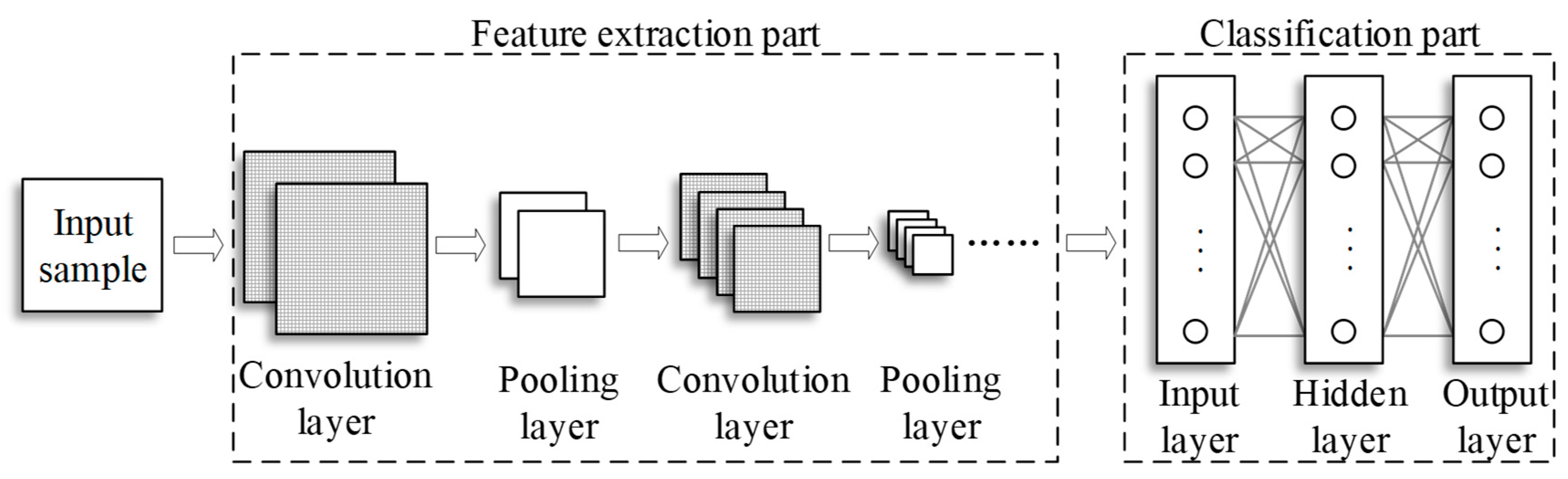
Convolutional Neural Networks (CNN) [28,29,30,31,32] contains two modules of feature extraction and classifier, in which the weights are updated continuously with the iterative process in training. The feature extraction neural network is mainly composed of multiple convolution layers and pooling layers. The main function of a convolution layer is to convolute the input signals to generate feature maps. The pooling layer merges adjacent data and compresses data dimensions. The neural network classifies the input signals according to final features extracted by the neural network. The CNN structure is shown in Figure 1.
2.1.1. Convolution Layer
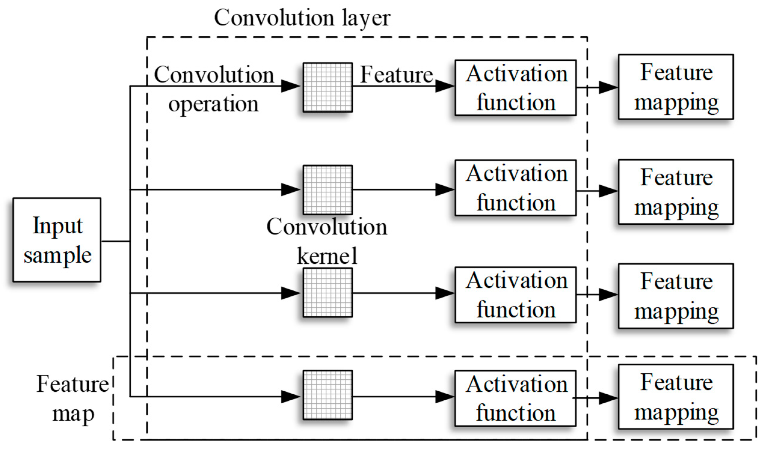
The convolution layer consists of several feature maps, and the number of output features depends on the number of feature maps. Each feature map performs the following operations on the input signal: The convolution operation is performed on the input sample with convolution kernel. Results are processed with activation functions, and feature mappings are output. The convolutional layer structure is shown in Figure 2.
The convolution core is a two-dimensional matrix which can be expressed by numerical or gray pixels, typically 5 × 5 or 3 × 3 in size. The convolution kernel is continuously updated with the number of iterations during the training process. This process can be compared with the weight update process of the ordinary neural network.
Given the input sample size and convolution kernel size, the feature size can be expressed by Equation (1). represents that the input sample is a matrix of size i × j; represents a convolution kernel size of q × q. Therefore, the feature size is . h denotes the sliding step size of the convolution kernel on the sample.
If the sliding step is always assumed to be 1, the convolution operation can be expressed by Equation (2). is the input sample; is the convolution kernel; and F(n,m) is the element value of the nth row and mth column of the feature mapping.
The value of each element in the feature mapping depends on whether the image resources match the shape of the convolution kernels [33].
Activation is to modify features, shield some smaller values of features, improve the sparsity of networks, reduce the interdependence of parameters, and alleviate the problem of over-fitting. In this study, SIGMOD is used for the activation of CNN. The expression of the function is shown in Equation (3).
2.1.2. Pooling Layer
The pooling layer is a scaling mapping of the output of the previous convolution layer. It combines adjacent pixels of the input into a single representative value, which can reduce the size of the feature and parameters of the network, and compensate for the objects deviating from the center and tilting in the sample [34]. The commonly used pooling operators have max pooling and average pooling. The formulaic expressions are shown in Equations (4) and (5). a(u,v) represents the value of the uth row and the vth column in the input matrix of the pooling layer; p(i,j) represents the value of the ith row and jth column in the output matrix of the pooling layer; and w is the boundary value of the participating pooled region.
2.1.3. Classification Network
In this study, classical BP (Back Propagation) neural network is used as a classifier. The BP neural network is a multi-layer feedforward network which is trained by error back propagation. It contains a forward propagation of signals and a back propagation of errors. The gradient descent method is the basic idea of the classical BP neural network and it uses the gradient search technique to minimize the mean square error between the actual output value of the network and the expected output value.
2.2. AutoEncoder
AutoEncoder (AE) is an artificial neural network used to reproduce the input signal as much as possible. It has a good ability to learn data characteristics. The essence of AE is to find a set of optimal weights (or vectors) to solve the projection of input data on weights, and then to get coding [35,36]. The basic structure is shown in Figure 3. It consists of an encoder and a decoder. The former one compresses the data and extracts the features, while the later one reconstructs the input signal. AE is trained by the error between the original input and the reconstructed input, and weights of neurons are adjusted by the criterion of minimizing the loss function of Equation (6) in multiple iterations. X is the input signal; W is the encoding; U is the decoding weight; Φ is the nonlinear activation function; J is the neuron weight adjustment function; R is the regularization function; and λ is the regularization coefficient.
The reconstruction error converges to the threshold range, and the features extracted by the encoder can express data characteristics well. The advantage of AE is that it does not depend on any expertise, but only pays attention to the characteristics of the input sample. The extracted features can restore the original sample to the greatest extent. The whole process can be carried out under the premise that the original data has no classification label. Moreover, the whole process does not require any manual intervention to further increase automation.
3. Self-Supervised Voltage Sag Source Identification Method Based on CNN
Based on the basic principle and main structure of AE, CNN and BP neural network, the convolution layer and pooling layer were used to extract features which were then classified by the BP classification network. No correct labeling of training samples was needed throughout the training process for supervision. Instead, the self-supervised training was carried out by the error between the reconstructed samples and the input samples. The trained system can extract features and identify sag sources on the input voltage sag waveform samples [37,38]. The structure of the self-supervised voltage sag source identification method based on CNN is shown in Figure 4.
3.1. Data Preprocessing
Step 1: The time-domain monitoring signals of various types of voltage sags can be obtained by using the voltage sag monitoring system.
Step 2: Each sag is classified in advance according to the type of voltage sag sources.
Step 3: All signals are resampled and the length of the waveform sequence is unified.
Step 4: Samples are normalized, and each sample is arranged into a two-dimensional matrix in a three-phase order, with each element in [0,1].
3.2. Extraction of Voltage Sag Waveform Characteristics
Step 1: Based on the basic principle and main structure of AE, the CNN model is embedded in the encoder, and a convolutional encoder is constructed to extract characteristics of voltage sag waveform.
Step 2: The pre-processed training samples are input into the convolution coder and convoluted with the convolution core in the convolution layer.
Step 3: The SIGMOD function is used as the activation function of CNN to get the corresponding feature mappings.
Step 4: Sizes of features are reduced through the pooling layer to compensate for the depression of the voltage sag data deviating from the center, and the corresponding final features are obtained.
Step 5: The obtained features are reconstructed by a convolutional decoder, and the convolution kernel and convolutional decoder in the convolutional layer are trained in the iterative process by the reconstruction error between the reconstructed sample and the input sample.
Step 6: Finally, good features which can accurately reflect the characteristics of voltage sag waveform are obtained.
3.3. Voltage Sag Source Identification
Step 1: BP neural network is constructed as the classification model in this study.
Step 2: An initial classification label of 1 × N (N is the number of BP neural network output layer units) can be obtained by inputting the features obtained by the above method into the classification network.
The number of BP neural network output layer units depends on the total number of categories of expected results. The label is meaningless without supervised iteration.
Step 3: According to the actual waveforms of various voltage sags, the standard sample waveforms of all kinds of sags are fitted. Each element in the label is regarded as the corresponding weight of each standard waveform. The reconstructed samples are constructed by accumulating the standard samples under the corresponding weights. This is shown in Equation (7). RSn is the reconstructed sample waveform, Wn is the elements in the tag matrix, Sn is the standard sample waveform, N is the total number of voltage sag source categories, and n is the current sag category.
Step 4: According to the reconstruction error between the original input sample and the reconstructed sample, the classification network is trained in the process of reverse propagation. After several iterations, the mean square error between the reconstructed sample and the original sample is minimized.
This transforms the problem of voltage sag source identification into a problem to recognize the optimal weight in the case where a fixed set of standard waveforms is used to represent the waveform to be identified. The back-propagation training process of the network is supervised by the reconstruction error, and the reconstructed samples are updated in each iteration to gradually approach the input samples.
Step 5: After training, the classification network determines the type of sag corresponding to the largest element in the classification label matrix, thus realizing the identification of voltage sag source.
4. Indicators for Model Evaluation
To evaluate the classification performance of CNN after each iteration under different parameters, an index describing the distance between the output results of each type of sag sample is defined in this study, which is named as the Degree of Discreteness of Classification Label (D). It is used to evaluate the impact of η1, η2 and maximum iteration number on CNN model.
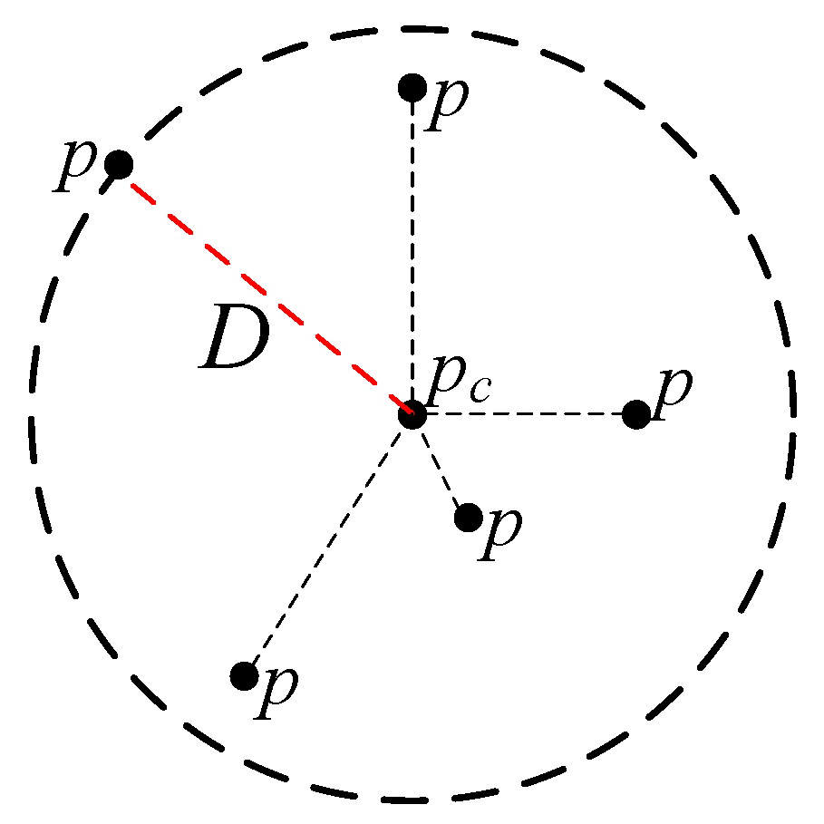
Each label can be considered as an N-dimensional vector, and the value of N depends on the total number of label categories. D is defined as the maximum distance between all label-vectors and center label-vectors. The expression of D is shown in Equation (8). The selection principle of center label-vectors (pvc) is shown in Equation (9).
where u is the total number of categories of data; n is the number of samples of the same type; v indicates that the current label distance of the vth class is being calculated; pvm, pvi, and pvj are the label vectors of the mth, ith, and jth waveforms in the vth sample waveform, respectively; pvc is the center label-vectors in the vth class. The norms used above are described below. If , , .
The principle of D is shown in Figure 5. In the figure, p represents the label-vectors; pc is the minimum label vectors according to the sum of all label distances except itself, that is, the center label-vectors. The distance labeled by red lines is the maximum distance between all label-vectors and the center label-vectors, which is equal to D. Generally, it is hoped that the classification labels of the same class of data after classification are as close as possible. Therefore, the value of D is negatively correlated with the classification effect of the network.
5. Result Analysis
5.1. Voltage Sag Type Classification and Data Preprocessing
Induction motor starting, transformer switching and short-circuit faults are the main causes of voltage sag. The voltage sag waveforms caused by different types of short-circuit faults, such as single-phase grounding, two-phase short-circuit and three-phase short-circuit, are also different. The above voltage sags can be divided into nine types: motor starting, transformer switching, three-phase short circuit, single-phase grounding (including A-phase grounding, B-phase grounding, C-phase grounding) as well as two-phase short circuit (including AB-phase short circuit, BC-phase short circuit and CA-phase short circuit).
The processor used in this computer was Intel(R) Celeron(R) 2957U @ 1.4G Hz 1.40 GHz. The data used in this example were all real-time monitoring data. According to monitoring data, the standard sample waveforms of nine types of sags were established and recorded as S1, S2 … S9, respectively (Table 1).
After preprocessing, each phase of the three-phase voltage was treated as a row, and each sample was normalized as a 2-D matrix of 3 × 27 with each element in [0,1]. Each row of data was repeated three times to obtain a 9 × 27 sample matrix, aiming to realize more convolution operations on the convolution kernel and extract characteristics of samples fully. Table 2 shows the typical voltage sags after graying.
5.2. Model Establishment and Optimal Parameter Selection
In the present study, a self-supervised CNN model was built on the basis of the classical three-layer CNN model structure. Since the input is a 9 × 27 two-dimensional matrix, the input layer contains 9 × 27 units. The CNN network for feature extraction consists of one convolution layer and one pooling layer. The convolution layer is composed of 16, 3 × 3-section convolution kernels, and the output of the convolutional layer is activated by the SIGMOD function and enters the pooling layer. The pooling layer uses an average pooling of 1 × 5 sub-matrices to output 16, 7 × 5 final feature matrices. The output of the feature extraction network is transformed into a 1 × 560 one-dimensional matrix input transition layer as the input layer of the classification network. The transition layer contains no other operations. The classification network of the model consists of one implicit layer and one hidden layer. The hidden layer has 100 units and uses a SIGMOD activation function. The number of output layer units is equal to the number of voltage sag source categories. In the case study, the output layer has nine units since the voltage sag source is divided into nine categories according to the fault phase. The constructed self-supervised CNN model is a six-layer model. The structural framework is shown in Figure 6. The momentum parameters of the convolution feature extraction network and classification network are both taken as 1.
To select the maximum number of iterations, a simulation experiment based on the learning rate of the CNN feature extraction network (η1) and the learning rate of the BP classification network (η2), which can deal with the problem of voltage sag source identification, was carried out firstly to select the best parameters for the above model. The maximum number of iterations was continuously adjusted to calculate D of the final result under different learning rates. The appropriate maximum number of iterations, η1 and η2, were selected by comparing the size of D. The simulation results are shown in Figure 7.
Analysis of the results in the graph showed that as the maximum number of iterations increases, D decreased gradually to a minimum. When the maximum number of iterations was 75, D was less than 1 when η1 ≥ 0.5 and η2 ≥ 0.5. Therefore, it set the maximum number of iterations as 75, η1 = 0.5, and η2 = 0.5 according to the simulation experiment.
5.3. Training Process of Feature Extraction
Three-hundred-and-sixty samples of measured voltage sags (including 40 S1, 40 S2, 40 S3, 40 S4, 40 S5, 40 S6, 40 S7, 40 S8, and 40 S9) were pre-processed and inputted into the CNN model for training. The status and output of each layer in a sag sample caused by inputting a phase B ground (Figure 8) are viewed in the case study.
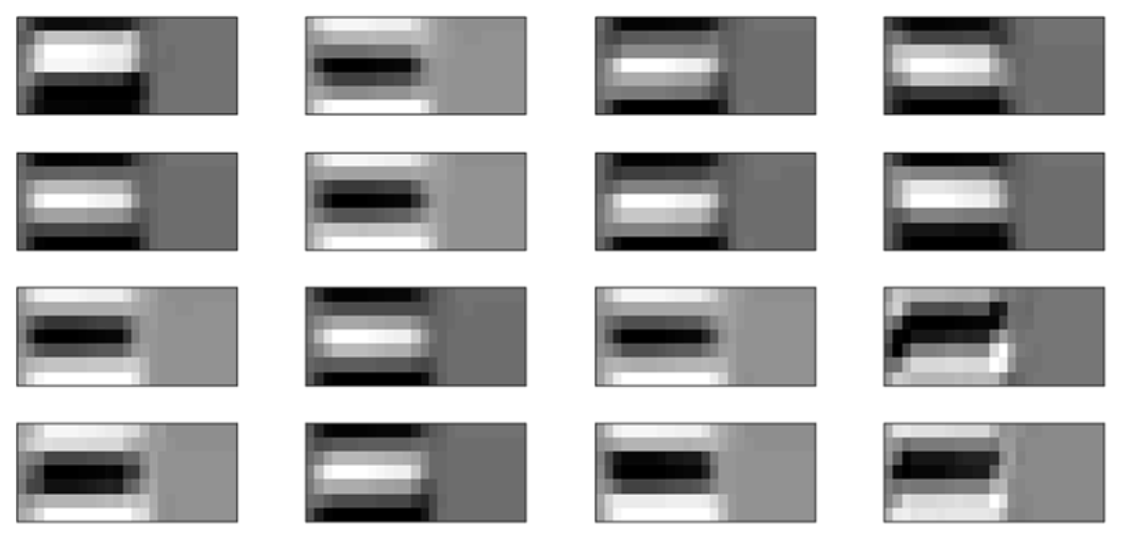
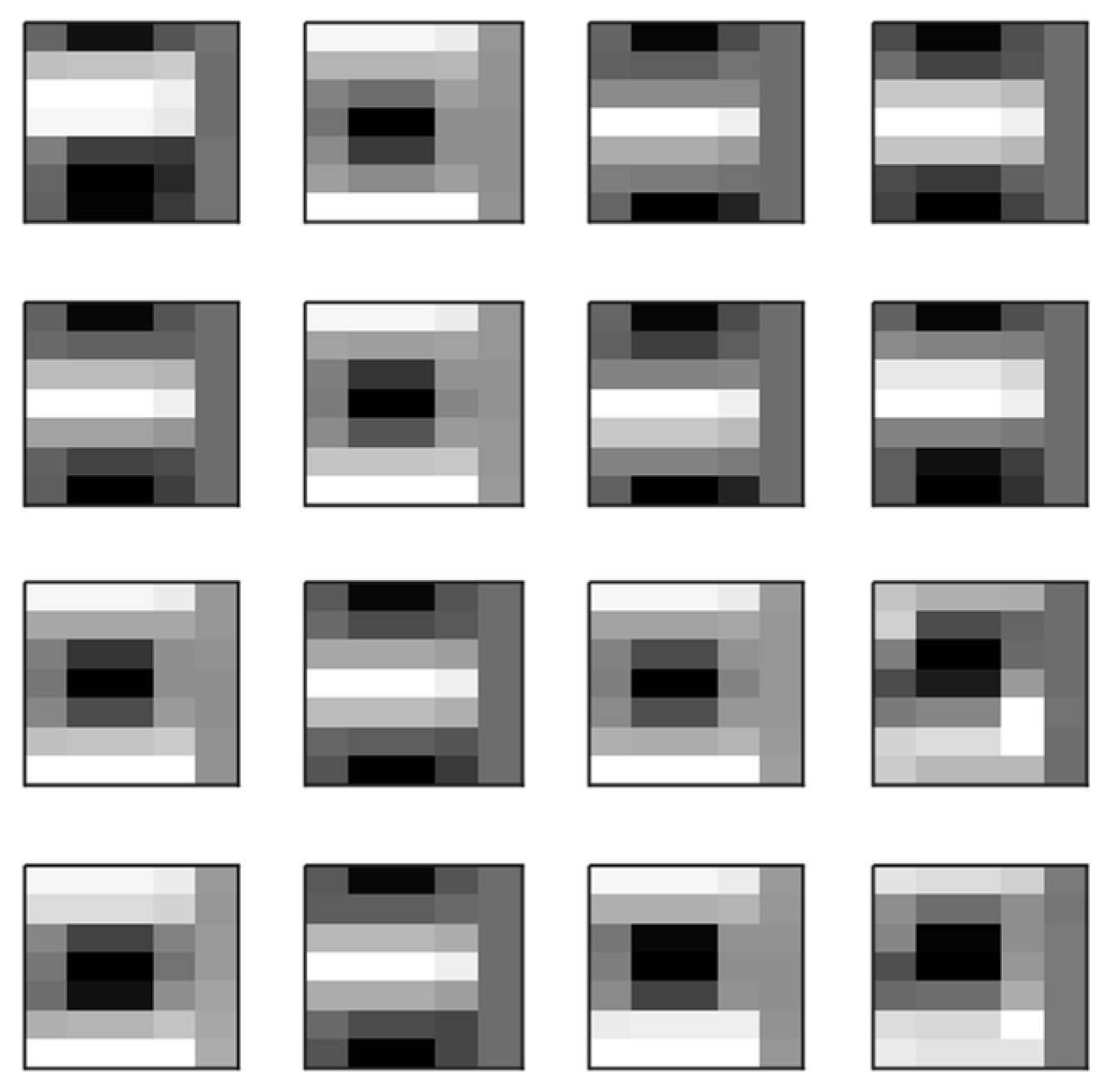
Both sample and convolutional kernels of the convolutional layer are subjected to a convolution operation and activated by SIGMOD to obtain feature mappings. The 16 feature mappings are shown in Figure 9. The feature mappings are compressed through the pooling layer and their offset centers are compensated. The model in this study used the average pooling to obtain the final features (Figure 10).
5.4. Results of Classification Labels
After training the classification network with 360 voltage sag waveform samples, 360 corresponding weight labels are obtained. The average weight labels of all kinds of sags are shown in Table 3. The maximum value of each line is bolded.
The temporary category corresponding to the largest element in the classification label matrix is deduced from Equation (7). The final identification result is determined based on the maximum element in the classification label. For example, the starting voltage sag of the motor corresponding to the standard sample S1 and W 1 in the weight label is the maximum value, which verifies the results in Table 3.
5.5. Results and Comparison with Other Methods
The test set 100 test samples (including 15 S1, 15 S2, 10 S3, 10 S4, 10 S5, 10 S6, 10 S7, 10 S8, and 10 S9) which are input into the model. The accuracy of the voltage sag source identification method based on the self-supervised CNN model is shown in Table 4.
To verify the superiority of this method, this example is compared with the method based on SVM in Reference [27]. The method in Reference [27] cannot distinguish the fault phase, so the comparison only involves the identification accuracy of sags. Results are shown in Table 5.
The experimental results showed that the accuracy of the sag source identification method using the SVM method is 83% and the accuracy of the method based on CNN is 97%. In Table 4, the identification accuracy of S3 to S9 reaches 100%. Among them, S3 represented a three-phase short circuit, S4 to S6 represented single-phase grounding, and S7-S9 represented a two-phase short circuit. They all belong to faults. Since the depression area is more obvious than other fault characteristics, it is easier to be distinguished. S3 is obviously different from other faults due to the lack of temporary rise characteristics. S4–S9 can be divided into different types according to the existence of sags in characteristics of each phase. In the extracted features, the information of each phase can be clearly obtained (Figure 9). However, the accuracy of motor starting and transformer switching is lower. The reason for this can be seen from Table 2, that S1 and S2 are very similar. Therefore, S1 and S2 can be easily distinguished from other types, but there is some confusion between them. Nevertheless, the total accuracy of the proposed method is still much higher than the method in Reference [27]. The accuracy of each type is lower than 90%. Moreover, the recognition accuracy reaches 100% in the judgment of the fault phase of asymmetric sags.
The time for each step in these two methods is shown in Table 6.
The most time-consuming step of SVM is feature extraction. Based on expert experiences, the method in Reference [27] set target features, including 60 equally distanced rms values, the remaining feature components, the 2nd harmonics magnitude, two odd harmonic magnitudes (5th and 9th) and the total harmonics distortion (THD) with respect to the fundamental. Later, the extracted features are input into SVM for training. The proposed method needs neither a label of training samples nor separated feature extraction. Feature extraction and machine training were implemented simultaneously. Therefore, the time for machine training is much longer than that for training SVM. These prove that the proposed method is simpler and claims a significantly shorter running time.
6. Conclusions
In this paper, a self-supervised voltage sag source identification method based on CNN is proposed. Its superiority in feature extraction and sag source identification are verified by a case study.
According to the analysis of the principle of the self-supervised CNN model and the results of practical examples, the self-supervised voltage sag source identification method based on CNN has some advantages:
- (1)
- Based on the structure of the convolutional neural network, the convolution operation of the convolution layer and the pooling operation of the pooling layer are used to extract the voltage sag feature. The problem that artificial feature extraction relies too much on expertise and is highly sensitive to unknown features is solved by transforming manual feature extraction into automatic feature extraction. This has no universality.
- (2)
- The self-supervised training process does not need to input a large number of training sets and correct labels in advance. Different from the traditional method, this self-supervised training process can identify unknown sag waveform correctly. It is more applicable to meet requirements of the sag source identification on timeliness, practicability, diversity, and versatility in the context of modern big data.
- (3)
- This method transforms three-phase waveform samples into a two-dimensional matrix input classification model instead of a one-dimensional matrix input. This preserves the information of different faults, and can expand the sag classes to nine categories, thus realizing the fault phase identification in three-phase asymmetric faults.
- (4)
- Compared with the SVM method, the self-supervised voltage sag source identification method based on CNN is proved to have a higher accuracy (97%) in the identification of measured sag data.
Author Contributions
Data curation, C.Z.; writing—original draft preparation, D.L.; writing—review and editing, H.S.; supervision, F.M.; project administration, J.Z.
Funding
This research received no external funding.
Conflicts of Interest
The authors declare no conflicts of interest.
References
- Khatri, N.; Jain, A.; Kumar, V.; Joshi, R.R. Voltage sag assessment with respect to sensitivity of adjustable speed drives in distributed generation environment. In Proceedings of the 2015 International Conference on Computer, Communication and Control (IC4), Indore, India, 10–12 September 2015; pp. 1–6. [Google Scholar]
- Wang, Z.; Guo, X.; Li, J.; Wang, X. Impact of Voltage Sags on Electric-Vehicle Charger and Critical Voltage Sag Determination. IEEE Trans. Power Deliv. 2016, 31, 1397–1399. [Google Scholar] [CrossRef]
- Weldemariam, L.; Cuk, V.; Cobben, S.; Waes, J.V. Regulation and classification of voltage dips. Cired Open Access Proc. J. 2017, 2017, 832–836. [Google Scholar] [CrossRef]
- McGranaghan, M.F.; Mueller, D.R.; Samotyj, M.J. Voltage sags in industrial systems. IEEE Trans. Ind. Appl. 1993, 29, 397–403. [Google Scholar] [CrossRef]
- López, M.A.G.; de Vicuña, J.L.G.; Miret, J.; Castilla, M.; Guzmán, R. Control Strategy for Grid-Connected Three-Phase Inverters During Voltage Sags to Meet Grid Codes and to Maximize Power Delivery Capability. IEEE Trans. Power Electron. 2018, 33, 9360–9374. [Google Scholar] [CrossRef]
- Liao, H.; Milanović, J.V.; Rodrigues, M.; Shenfield, A. Voltage Sag Estimation in Sparsely Monitored Power Systems Based on Deep Learning and System Area Mapping. IEEE Trans. Power Deliv. 2018, 33, 3162–3172. [Google Scholar] [CrossRef]
- Bagheri, A.; Bollen, M. Developments in voltage dip research and its applications, 2005–2015. In Proceedings of the 2016 17th International Conference on Harmonics and Quality of Power (ICHQP), Belo Horizonte, Brazil, 16–19 October 2016; pp. 48–54. [Google Scholar]
- Becnel, C.L. Maintaining Process Continuity During Voltage Dips. IEEE Trans. Ind. Appl. 1982, 4, 324–328. [Google Scholar] [CrossRef]
- Conrad, L.; Little, K.; Grigg, C. Predicting and preventing problems associated with remote fault-clearing voltage dips. IEEE Trans. Ind. Appl. 1991, 27, 167–172. [Google Scholar] [CrossRef]
- Bollen, M.H.J. Characterisation of voltage sags experienced by three-phase adjustable-speed drives. IEEE Trans. Power Deliv. 1997, 12, 1666–1671. [Google Scholar] [CrossRef]
- Lidong, Z.; Bollen, M.H.J. Characteristic of voltage dips (sags) in power systems. IEEE Trans. Power Deliv. 2000, 15, 827–832. [Google Scholar] [CrossRef]
- Madrigal, M.; Rocha, B.H. A Contribution for Characterizing Measured Three-Phase Unbalanced Voltage Sags Algorithm. IEEE Trans. Power Deliv. 2007, 22, 1885–1890. [Google Scholar] [CrossRef]
- Shareef, H.; Mohamed, A. An alternative voltage sag source identification method utilizing radial basis function network. In Proceedings of the 22nd International Conference and Exhibition on Electricity Distribution (CIRED 2013), Stockholm, Sweden, 10–13 June 2013; pp. 1–4. [Google Scholar]
- Gaouda, A.M.; Salama, M.M.A.; Sultan, M.R.; Chikhani, A.Y. Application of multiresolution signal decomposition for monitoring short-duration variations in distribution systems. IEEE Trans. Power Deliv. 2000, 15, 478–485. [Google Scholar] [CrossRef]
- Ignatova, V.; Granjon, P.; Bacha, S.; Dumas, F. Classification and characterization of three phase voltage dips by space vector methodology. In Proceedings of the 2005 International Conference on Future Power Systems, Amsterdam, The Netherlands, 18 November 2005; p. 6. [Google Scholar]
- Karimi, M.; Mokhtari, H.; Iravani, M.R. Wavelet based on-line disturbance detection for power quality applications. IEEE Trans. Power Deliv. 2000, 15, 1212–1220. [Google Scholar] [CrossRef]
- Moussa, S.A. Distributed generation unit allocation utilizing expert system with reliability and voltage sag consideration. In Proceedings of the 2015 Long Island Systems, Applications and Technology, Farmingdale, NY, USA, 1 May 2015; pp. 1–5. [Google Scholar]
- Styvaktakis, E.; Bollen, M.H.J.; Gu, I.Y.H. Expert system for classification and analysis of power system events. IEEE Trans. Power Deliv. 2002, 17, 423–428. [Google Scholar] [CrossRef]
- Gu, I.Y.H.; Ernberg, N.; Styvaktakis, E.; Bollen, M.H.J. A statistical-based sequential method for fast online detection of fault-induced voltage dips. IEEE Trans. Power Deliv. 2004, 19, 497–504. [Google Scholar] [CrossRef]
- Huang, J.S.; Negnevitsky, M.; Nguyen, D.T. A neural-fuzzy classifier for recognition of power quality disturbances. In Proceedings of the 2002 IEEE Power Engineering Society Winter Meeting, Conference Proceedings (Cat. No.02CH37309), New York, NY, USA, 27–31 January 2002; Volume 2, p. 930. [Google Scholar]
- Singh, M.; Chacko, S.T.; Zadgaonkar, A.S. Detection of voltage sag by artificial neural network and mitigation using DSTATCOM. In Proceedings of the 2012 2nd International Conference on Power, Control and Embedded Systems, Allahabad, India, 17–19 December 2012; pp. 1–5. [Google Scholar]
- Valtierra-Rodriguez, M.; Romero-Troncoso, R.D.J.; Osornio-Rios, R.A.; Garcia-Perez, A. Detection and Classification of Single and Combined Power Quality Disturbances Using Neural Networks. IEEE Trans. Ind. Electron. 2014, 61, 2473–2482. [Google Scholar] [CrossRef]
- Wijayakulasooriya, J.V.; Putrus, G.A.; Minns, P.D. Electric power quality disturbance classification using self-adapting artificial neural networks. IEE Proc. Gener. Transm. Distrib. 2002, 149, 98–101. [Google Scholar] [CrossRef]
- Moulin, L.S.; da Silva, A.P.A.; El-Sharkawi, M.A.; Marks, R.J. Support vector machines for transient stability analysis of large-scale power systems. IEEE Trans. Power Syst. 2004, 19, 818–825. [Google Scholar] [CrossRef]
- Thukaram, D.; Khincha, H.P.; Vijaynarasimha, H.P. Artificial neural network and support vector Machine approach for locating faults in radial distribution systems. IEEE Trans. Power Deliv. 2005, 20, 710–721. [Google Scholar] [CrossRef]
- He, H.; Starzyk, J.A. A self-organizing learning array system for power quality classification based on wavelet transform. IEEE Trans. Power Deliv. 2006, 21, 286–295. [Google Scholar] [CrossRef]
- Axelberg, P.G.V.; Gu, I.Y.; Bollen, M.H.J. Support Vector Machine for Classification of Voltage Disturbances. IEEE Trans. Power Deliv. 2007, 22, 1297–1303. [Google Scholar] [CrossRef]
- Ciresan, D.C.; Meier, U.; Gambardella, L.M.; Schmidhuber, J. Convolutional Neural Network Committees for Handwritten Character Classification. In Proceedings of the 2011 International Conference on Document Analysis and Recognition, Beijing, China, 18–21 September 2011; pp. 1135–1139. [Google Scholar]
- Ming, L.; Xiaolin, H. Recurrent convolutional neural network for object recognition. In Proceedings of the 2015 IEEE Conference on Computer Vision and Pattern Recognition (CVPR), Boston, MA, USA, 7–12 June 2015; pp. 3367–3375. [Google Scholar]
- Guo, T.; Dong, J.; Li, H.; Gao, Y. Simple convolutional neural network on image classification. In Proceedings of the 2017 IEEE 2nd International Conference on Big Data Analysis (ICBDA), Beijing, China, 10–12 March 2017; pp. 721–724. [Google Scholar]
- Hamalainen, A.; Henriksson, J. Convolutional decoding using recurrent neural networks. In Proceedings of the IJCNN’99, International Joint Conference on Neural Networks, Proceedings (Cat. No. 99CH36339), Washington, DC, USA, 10–16 July 1999; Volume 5, pp. 3323–3327. [Google Scholar]
- Henriksson, J. Novel use of channel information in a neural convolutional decoder. In Proceedings of the IEEE-INNS-ENNS International Joint Conference on Neural Networks, IJCNN 2000, Neural Computing: New Challenges and Perspectives for the New Millennium, Como, Italy, 27 July 2000; Volume 5, pp. 337–342. [Google Scholar]
- Oquab, M.; Bottou, L.; Laptev, I.; Sivic, J. Learning and Transferring Mid-level Image Representations Using Convolutional Neural Networks. In Proceedings of the 2014 IEEE Conference on Computer Vision and Pattern Recognition, Columbus, OH, USA, 23–28 June 2014; pp. 1717–1724. [Google Scholar]
- Liu, L.; Shen, C.; Hengel, A.V.D. The treasure beneath convolutional layers: Cross-convolutional-layer pooling for image classification. In Proceedings of the 2015 IEEE Conference on Computer Vision and Pattern Recognition (CVPR), Boston, MA, USA, 7–12 June 2015; pp. 4749–4757. [Google Scholar]
- Chen, Z.; Yeo, C.K.; Lee, B.S.; Lau, C.T. Autoencoder-based network anomaly detection. In Proceedings of the 2018 Wireless Telecommunications Symposium (WTS), Phoenix, AZ, USA, 17–20 April 2018; pp. 1–5. [Google Scholar]
- Janod, K.; Morchid, M.; Dufour, R.; Linarès, G.; Mori, R.D. Denoised Bottleneck Features from Deep Autoencoders for Telephone Conversation Analysis. IEEE/ACM Trans. Audio Speech Lang. Process. 2017, 25, 1809–1820. [Google Scholar] [CrossRef]
- Mohan, N.; Soman, K.P.; Vinayakumar, R. Deep power: Deep learning architectures for power quality disturbances classification. In Proceedings of the 2017 International Conference on Technological Advancements in Power and Energy (TAP Energy), Kollam, India, 21–23 December 2017; pp. 1–6. [Google Scholar]
- Balouji, E.; Salor, O. Classification of power quality events using deep learning on event images. In Proceedings of the 2017 3rd International Conference on Pattern Recognition and Image Analysis (IPRIA), Shahrekord, Iran, 19–20 April 2017; pp. 216–221. [Google Scholar]
Figure 1.
CNN structure.

Figure 2.
Convolutional layer structure.

Figure 3.
AE model structure.

Figure 4.
Self-supervised Voltage Sag Source Identification Method Based on CNN.

Figure 5.
The principle of Degree of Discreteness of Classification Label.

Figure 6.
Structural framework of self-supervised CNN model for case study.

Figure 7.
Degree of Discreteness of Classification Label under different iteration numbers and learning rates.
Figure 7.
Degree of Discreteness of Classification Label under different iteration numbers and learning rates.

Figure 8.
Sample of S5.

Figure 9.
Feature mappings.

Figure 10.
Final features after average pooling.


Table 1.
Standard sample for voltage sag category.
| Motor Starting (S1) | Transformer Switching (S2) | Three-Phase Short Circuit (S3) | |||
 |  |  | |||
| Single-Phase Grounding | A-phase (S4) |  | Two-Phase Short Circuit | BC-phase (S7) |  |
| B-phase (S5) |  | CA-phase (S8) |  | ||
| C-phase (S6) |  | AB-phase (S9) |  | ||
Table 2.
Grayscale image of voltage sag category.
| Motor starting (S1) | Transformer switching (S2) | Three-phase short circuit (S3) | |||
 |  |  | |||
| Single-phase grounding | A-phase (S4) |  | Two-Phase Short Circuit | BC-phase (S7) |  |
| B-phase (S5) |  | CA-phase (S8) |  | ||
| C-phase (S6) |  | AB-phase (S9) |  | ||
Table 3.
Average Classification Label for Various Types of Voltage Sag Sources.
| W1 | W2 | W3 | W4 | W5 | W6 | W7 | W8 | W9 | |
|---|---|---|---|---|---|---|---|---|---|
| S1 | 1.1866 | −0.1249 | −0.0758 | −0.1087 | −0.0930 | 0.1334 | −0.1383 | −0.0986 | −0.0483 |
| S2 | 0.1282 | 1.2409 | 0.0548 | −0.0056 | 0.1253 | 0.1135 | 0.0058 | 0.0051 | −0.1009 |
| S3 | −0.0264 | 0.0062 | 1.0661 | 0.0200 | 0.0198 | −0.0036 | −0.0239 | 0.0938 | −0.0409 |
| S4 | −0.0404 | 0.0843 | −0.0886 | 1.1396 | 0.1244 | 0.0633 | 0.0820 | −0.0460 | −0.1063 |
| S5 | 0.1132 | −0.0426 | −0.0715 | 0.0153 | 1.0610 | 0.0366 | −0.0559 | 0.0873 | 0.1234 |
| S6 | −0.0463 | 0.0136 | −0.0811 | 0.0192 | 0.0672 | 1.2245 | 0.1387 | 0.0716 | −0.0514 |
| S7 | −0.0904 | 0.0947 | −0.0894 | 0.0419 | −0.1175 | −0.0219 | 0.8073 | 0.0905 | −0.0923 |
| S8 | 0.0948 | −0.0484 | 0.0661 | −0.0338 | −0.0593 | −0.0082 | −0.1051 | 1.1994 | 0.0963 |
| S9 | 0.1158 | 0.0776 | −0.0302 | −0.0459 | 0.1108 | −0.0832 | 0.0543 | 0.0752 | 0.9386 |
Table 4.
The accuracy of voltage sag source identification method based on self-supervised CNN model.
Table 4.
The accuracy of voltage sag source identification method based on self-supervised CNN model.
| The Class of Voltage Sag Source | The Amount of Test Samples | The Number of Correct Results | Accuracy |
|---|---|---|---|
| S1 | 15 | 14 | 93.33% |
| S2 | 15 | 13 | 86.67% |
| S3 | 10 | 10 | 100% |
| S4 | 10 | 10 | 100% |
| S5 | 10 | 10 | 100% |
| S6 | 10 | 10 | 100% |
| S7 | 10 | 10 | 100% |
| S8 | 10 | 10 | 100% |
| S9 | 10 | 10 | 100% |
| Total | 100 | 97 | 97% |
Table 5.
Accuracy of different voltage sag source identification methods.
| The Class of Voltage Sag Source | The Amount of Test Samples | SVM | CNN |
|---|---|---|---|
| Motor starting | 15 | 80% | 93.33% |
| Transformer switching | 15 | 73.33% | 86.67% |
| Three-phase short circuit | 10 | 80% | 100% |
| Single-phase grounding | 30 | 83.33% | 100% |
| Two-phase short circuit | 30 | 86.67% | 100% |
| Total | 100 | 83% | 97% |
Table 6.
The time for each step in these two methods.
| Time of Each Step | Preproc-Essing Data | Obtaining Correct Label | Extracting Features | Training Machines with Training Samples | Verifying Accuracy with Test Samples | Total Time |
|---|---|---|---|---|---|---|
| SVM | 21.96 s | 0.74 s | 1188.39 s | 8.94 s | 0.08 s | 1214.11 s |
| CNN | 21.96 s | / | / | 35.32 s | 0.11 s | 57.39 s |
© 2019 by the authors. Licensee MDPI, Basel, Switzerland. This article is an open access article distributed under the terms and conditions of the Creative Commons Attribution (CC BY) license (http://creativecommons.org/licenses/by/4.0/).
Share and Cite
MDPI and ACS Style
Li, D.; Mei, F.; Zhang, C.; Sha, H.; Zheng, J. Self-Supervised Voltage Sag Source Identification Method Based on CNN. Energies 2019, 12, 1059. https://doi.org/10.3390/en12061059
AMA Style
Li D, Mei F, Zhang C, Sha H, Zheng J. Self-Supervised Voltage Sag Source Identification Method Based on CNN. Energies. 2019; 12(6):1059. https://doi.org/10.3390/en12061059
Chicago/Turabian StyleLi, Danqi, Fei Mei, Chenyu Zhang, Haoyuan Sha, and Jianyong Zheng. 2019. "Self-Supervised Voltage Sag Source Identification Method Based on CNN" Energies 12, no. 6: 1059. https://doi.org/10.3390/en12061059
Note that from the first issue of 2016, this journal uses article numbers instead of page numbers. See further details here.