Energy Regulator Supply Restoration Time


Abstract
1. Introduction
2. Input Parameters
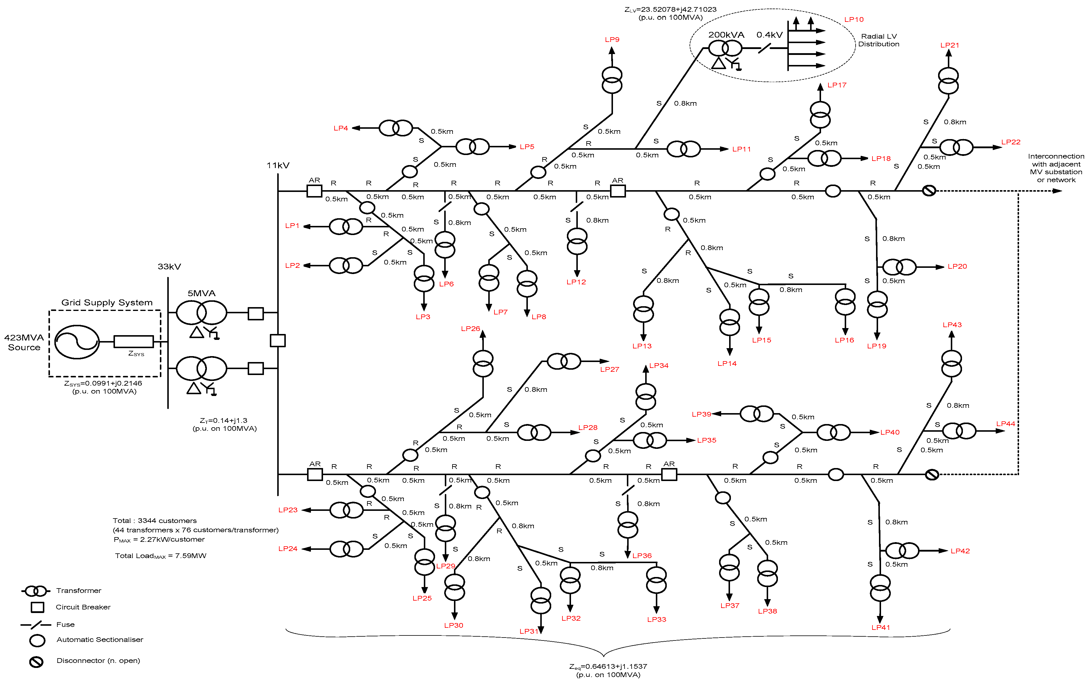
2.1. Suburban MV Network
2.2. Mean Fault Rates and Mean Time to Repair (MTTR)
2.3. Fault Types
2.4. Guaranteed Standard of Performance
3. Reliability Methodologies
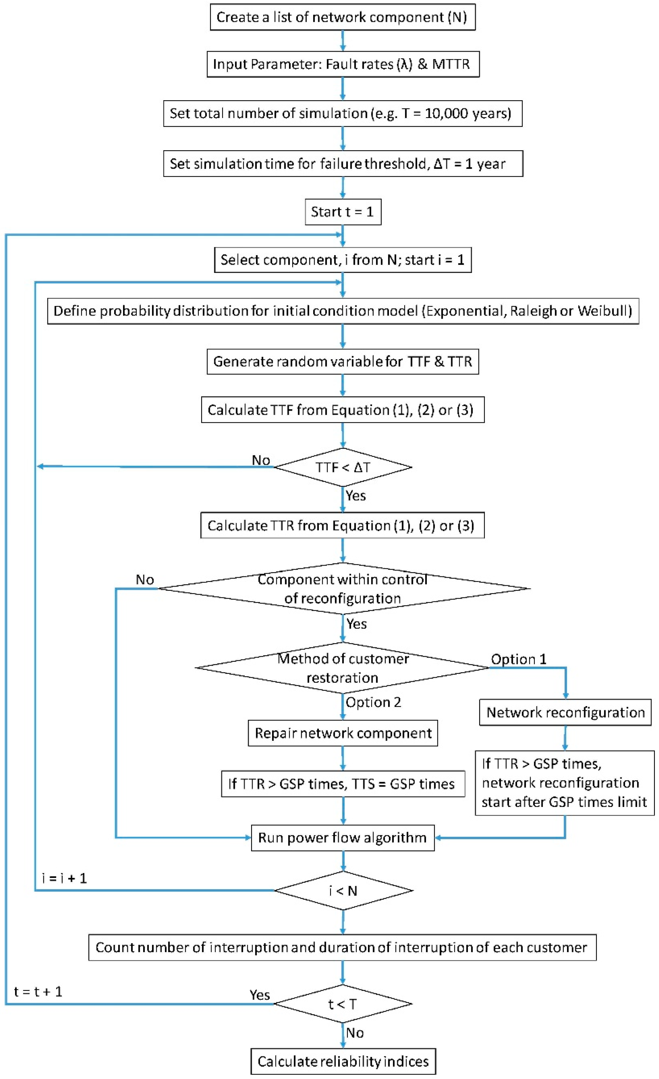
3.1. Monte Carlo Simulation (MCS) Procedures
3.2. Considered Scenarios
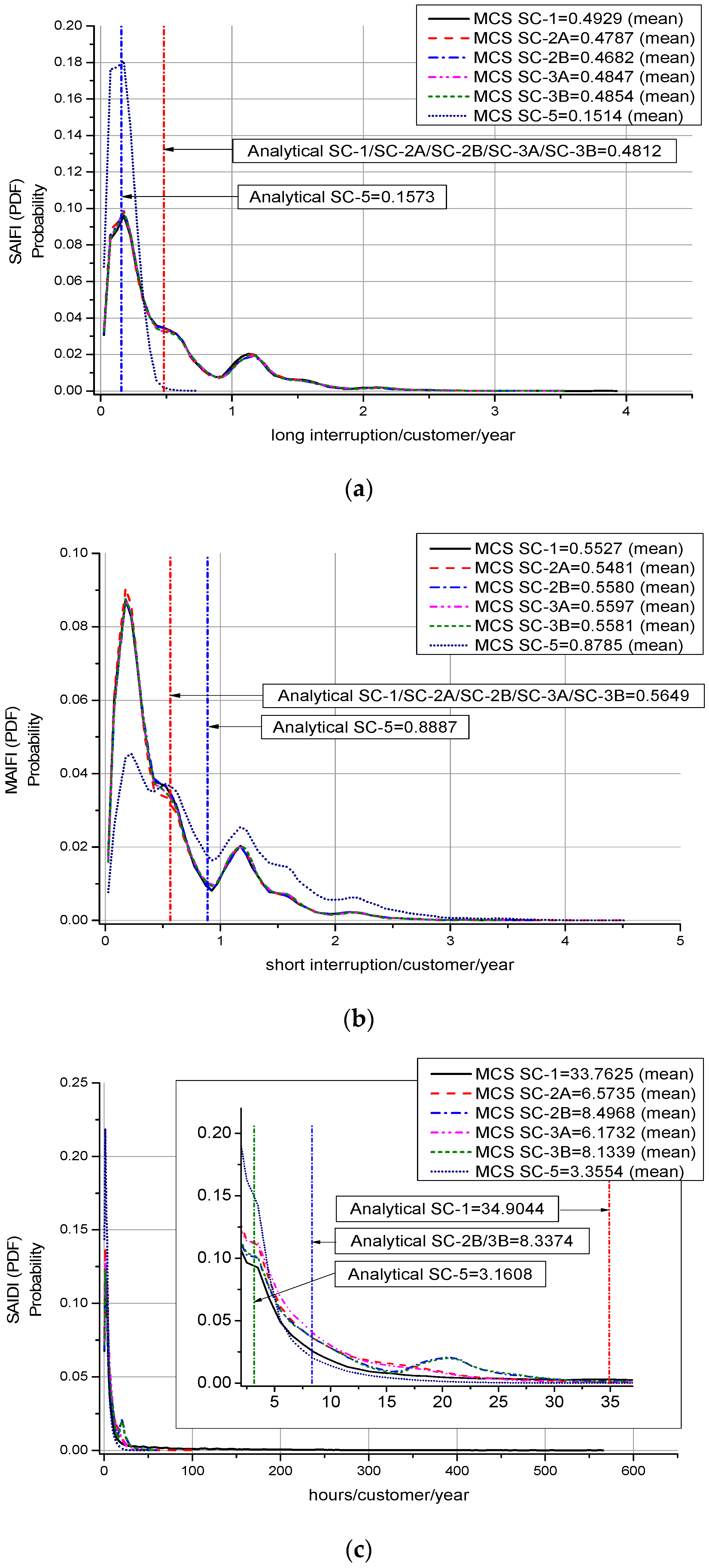
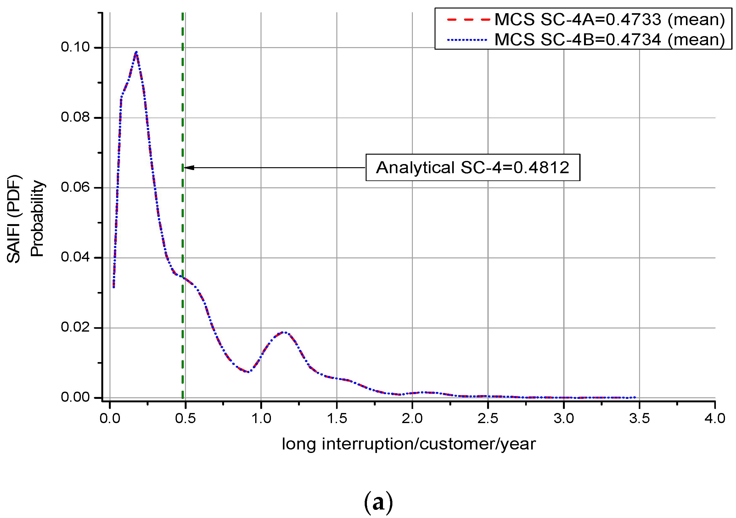
4. Reliability Performance Results
5. Discussion
6. Conclusions
Author Contributions
Funding
Acknowledgments
Conflicts of Interest
References
- The Electricity Standard of Performance Regulations Statutory Instruments. Standard No.698; Office of Gas and Electricity Markets (OFGEM): London, UK, 2010.
- CEER. 6th CEER Benchmarking Report on the Quality of Electricity and Gas Supply 2016; Report Contin. Electricity Supply; CEER (Council of European Energy Regulators): Brussels, Belgium, 2016. [Google Scholar]
- Engineering Recommendation P2/6 Security of Supply; Energy Networks Association (ENA): London, UK, 2005; pp. 1–13.
- Liu, K.Y.; Sheng, W.; Liu, Y.; Meng, X. A network reconfiguration method considering data uncertainties in smart distribution networks. Energies 2017, 10, 618. [Google Scholar]
- Wen, J.; Tan, Y.; Jiang, L. A reconfiguration strategy of distribution networks considering node importance. PLoS ONE 2016, 11, 1–20. [Google Scholar] [CrossRef] [PubMed]
- Flaih, F.; Lin, X.; Abd, M.; Dawoud, S.; Li, Z.; Adio, O. A New Method for Distribution Network Reconfiguration Analysis under Different Load Demands. Energies 2017, 10, 455. [Google Scholar] [CrossRef]
- Nguyen, T.T.; Truong, A.V.; Phung, T.A. A novel method based on adaptive cuckoo search for optimal network reconfiguration and distributed generation allocation in distribution network. Int. J. Electr. Power Energy Syst. 2016, 78, 801–815. [Google Scholar] [CrossRef]
- Adoghe, A.U.; Awosope, C.O.A.; Ekeh, J.C. Asset maintenance planning in electric power distribution network using statistical analysis of outage data. Int. J. Electr. Power Energy Syst. 2013, 47, 424–435. [Google Scholar] [CrossRef]
- Vale, Z.; Soares, J.; Lobo, C.; Canizes, B. Multi-criteria optimisation approach to increase the delivered power in radial distribution networks. IET Gener. Transm. Distrib. 2015, 9, 2565–2574. [Google Scholar]
- Usberti, F.L.; Lyra, C.; Cavellucci, C.; González, J.F.V. Hierarchical multiple criteria optimization of maintenance activities on power distribution networks. Ann. Oper. Res. 2015, 224, 171–192. [Google Scholar] [CrossRef]
- Zare, M.R.; Hooshmand, R.; Eshtehardiha, S.; Poodeh, M.B. Effect of Time-Variability Weather Conditions on the Reliability of Distribution Systems. In Proceedings of the 7th WSEAS International Conference on Electric Power Systems, High Voltages, Electric Machines, Venice, Italy, 21–23 November 2007; pp. 160–165. [Google Scholar]
- Carpaneto, E. Distribution system minimum loss reconfiguration in the Hyper-Cube Ant Colony Optimization framework. Electr. Power Syst. Res. 2008, 78, 2037–2045. [Google Scholar] [CrossRef]
- Fathabadi, H. Power distribution network reconfiguration for power loss minimization using novel dynamic fuzzy c-means (dFCM) clustering based ANN approach. Int. J. Electr. Power Energy Syst. 2016, 78, 96–107. [Google Scholar] [CrossRef]
- Shirmohammadi, D.; Hong, H.W. Reconfiguration of electric distribution networks for resistive line losses reduction. IEEE Trans. Power Deliv. 1989, 4, 1492–1498. [Google Scholar] [CrossRef]
- Kumar, K.S.; Jayabarathi, T. Power system reconfiguration and loss minimization for an distribution systems using bacterial foraging optimization algorithm. Int. J. Electr. Power Energy Syst. 2012, 36, 13–17. [Google Scholar] [CrossRef]
- Ferdavani, A.K.; Zin, A.A.M.; Khairuddin, A.; Naeini, M.M. Reconfiguration of Radial Electrical Distribution Network through Neighbor-Chain Updating method. In Proceedings of the TENCON 2011—2011 IEEE Region 10 Conference, Bali, Indonesia, 21–24 November 2011; pp. 991–994. [Google Scholar]
- Imran, A.M.; Kowsalya, M. A new power system reconfiguration scheme for power loss minimization and voltage profile enhancement using Fireworks Algorithm. Int. J. Electr. Power Energy Syst. 2014, 62, 312–322. [Google Scholar] [CrossRef]
- Shareef, H.; Ibrahim, A.A.; Salman, N.; Mohamed, A.; Ai, W.L. Power quality and reliability enhancement in distribution systems via optimum network reconfiguration by using quantum firefly algorithm. Int. J. Electr. Power Energy Syst. 2014, 58, 160–169. [Google Scholar] [CrossRef]
- Rajaram, R.; Kumar, K.S.; Rajasekar, N. Power system reconfiguration in a radial distribution network for reducing losses and to improve voltage profile using modified plant growth simulation algorithm with Distributed Generation (DG). Energy Rep. 2015, 1, 116–122. [Google Scholar] [CrossRef]
- Nguyen, T.T.; Truong, A.V. Distribution network reconfiguration for power loss minimization and voltage profile improvement using cuckoo search algorithm. Int. J. Electr. Power Energy Syst. 2015, 68, 233–242. [Google Scholar] [CrossRef]
- Gupta, N.; Swarnkar, A.; Niazi, K.R. Distribution network reconfiguration for power quality and reliability improvement using Genetic Algorithms. Int. J. Electr. Power Energy Syst. 2014, 54, 664–671. [Google Scholar] [CrossRef]
- Hernando-Gil, I.; Ilie, I.-S.; Collin, A.J.; Acosta, J.L.; Djokic, S.Z. Impact of DG and energy storage on distribution network reliability: A comparative analysis. In Proceedings of the 2012 IEEE International Energy Conference and Exhibition (ENERGYCON), Florence, Italy, 9–12 September 2012; pp. 605–611. [Google Scholar]
- Lakervi, E.; Holmes, E. Electricity Distribution Network Design. Available online: https://books.google.com.hk/books?hl=zh-TW&lr=&id=TpW28vHkE-0C&oi=fnd&pg=PR11&dq=Electricity+Distribution+Network+Design&ots=ppzWMReCr2&sig=_Kjze7swVrRLUPYoGwiMubQX4Qg&redir_esc=y#v=onepage&q=Electricity%20Distribution%20Network%20Design&f=false (accessed on 4 March 2019).
- Code of Practice for the Protection and Control of HV Circuits; CE Electric UK: Newcastle upon Tyne, UK, 2015; pp. 1–30.
- Charlesworth, D. Primary Network Design Manual; EON Central Network: Coventry, UK, 2007; pp. 1–118. [Google Scholar]
- Powergrid, N. Code of Practice for the Protection and Control of HV Circuits (DSS/007/010); Northern Powergrid: Newcastle upon Tyne, UK, 2011. [Google Scholar]
- Puret, C. MV Public Distribution Networks throughout the World; E/CT: Cheshire, UK, 1992. [Google Scholar]
- Guaranteed Standards of Performance for Metered Demand Customers of Electricity Distribution Companies in England, Wales & Scotland. Available online: https://www.google.com.hk/url?sa=t&rct=j&q=&esrc=s&source=web&cd=1&ved=2ahUKEwiEy-6phujgAhUyE6YKHWr7AFoQFjAAegQIABAC&url=https%3A%2F%2Fwww.ukpowernetworks.co.uk%2Finternet%2Fen%2Fabout-us%2Fdocuments%2FUKPN-DNO-NOR-Jan-2013-final-UKPN-branded.pdf&usg=AOvVaw24dnU4UsB7pt8jgUx_Fqrp (accessed on 4 March 2019).
- DRAKA Product Range Cable Specifications; Draka UK Limited: Eastleigh, UK, 2010.
- Specifications for Electricity Service and Distribution Cables for Use during the Installation of New Connections; Scottish & Southern Energy Power Distribution: Glasgow, UK, 2010.
- Information to Assist Third Party in the Design and Installation of New Secondary Substations for Adoption or Use by SSE Power Distribution; SSE Power Distribution: Glasgow, UK, 2007.
- Distribution Long Term Development Statement for the Years 2011/12 to 2015/16; SP Distribution and SP Manweb: Glasgow, UK, 2011.
- National System and Equipment Performance Report; Energy Networks Association (ENA): London, UK, 2010.
- Allan, R.; de Oliveira, M. Evaluating the reliability of electrical auxiliary systems in multi-unit generating stations. IEE Proc. C Gener. Transm. Distrib. 1980, 127, 65–71. [Google Scholar] [CrossRef]
- Stanek, E.; Venkata, S. Mine power system reliability. IEEE Trans. Ind. Appl. 1988, 24, 827–838. [Google Scholar] [CrossRef]
- Farag, A.; Wang, C.; Cheng, T. Failure analysis of composite dielectric of power capacitors in distribution systems. Electr. Power Syst. Res. 1998, 44, 117–126. [Google Scholar] [CrossRef]
- Office of Gas and Electricity Markets. The Performance of Networks Using Alternative Splitting Configurations; Final Report on Technical Steering Group Workstream; Office of Gas and Electricity Markets (OFGEM): London, UK, 2004.
- Roos, F.; Lindah, S. Distribution system component failure rates and repair times—An overview. In Proceedings of the Nordic Distribution and Asset Management Conference, Espoo, Finland, 23–24 August 2004. [Google Scholar]
- Anders, G.; Maciejewski, H. A comprehensive study of outage rates of air blast breakers. IEEE Trans. Power Syst. 2006, 21, 202–210. [Google Scholar] [CrossRef]
- Office of Gas and Electricity Markets. Review of Electricity Transmission Output Measures; Final Report; Office of Gas and Electricity Markets (OFGEM): London, UK, 2008.
- He, Y. Study and Analysis of Distribution Equipment Reliability Data; Elforsk AB: Stockholm, Sweden, 2010. [Google Scholar]
- Office of Gas and Electricity Markets (OFGEM). Electricity Distribution Quality of Service Report 2008/09; Office of Gas and Electricity Markets: London, UK, 2009.
- Billinton, R.; Allan, R. Reliability Evaluation of Power Systems, 2nd ed.; Springer: New York, NY, USA, 1996. [Google Scholar]
- Bie, Z.; Zhang, P.; Li, G.; Hua, B.; Meehan, M.; Wang, X. Reliability Evaluation of Active Distribution Systems Including Microgrids. IEEE Trans. Power Syst. 2012, 27, 2342–2350. [Google Scholar] [CrossRef]
- Arya, L.D.; Choube, S.C.; Arya, R.; Tiwary, A. Evaluation of reliability indices accounting omission of random repair time for distribution systems using Monte Carlo simulation. Int. J. Electr. Power Energy Syst. 2012, 42, 533–541. [Google Scholar] [CrossRef]
- Zhang, H.; Li, P. Probabilistic analysis for optimal power flow under uncertainty. IET Gener. Transm. Distrib. 2010, 4, 553. [Google Scholar] [CrossRef]
- Alvehag, K.; Söder, L. Risk-based method for distribution system reliability investment decisions under performance-based regulation. IET Gener. Transm. Distrib. 2011, 5, 1062. [Google Scholar] [CrossRef]
- Hadjsaid, N.; Sabonnadiere, J.-C. Electrical Distribution Networks; John Wiley & Sons: Hoboken, NJ, USA, 2013. [Google Scholar]
- Hribar, L.; Duka, D. Weibull distribution in modeling component faults. In Proceedings of the ELMAR-2010, Zadar, Croatia, 15–17 September 2010; pp. 183–186. [Google Scholar]
- Rubinstein, R.Y.; Kroese, D.P. Simulation and the Monte Carlo Method; John Wiley & Sons, Inc.: Hoboken, NJ, USA, 2016. [Google Scholar]


| Operating Voltage (kV) | Feeder Type | Id. | Cross Section (mm2) | Resistance/km | Reactance/km |
|---|---|---|---|---|---|
| (p.u. on 100 MVA) | |||||
| 11 | Overhead Lines or Mixed | R | 150 | 0.11259 | 0.18363 |
| S | 100 | 0.14658 | 0.26189 | ||
| 0.4 | D | 95 | 0.32 | 0.075 | |
| E | 50 | 0.443 | 0.076 | ||
| H | 95 | 0.32 | 0.085 | ||
| 0.23 | L | 35 | 0.851 | 0.041 | |
| Operating Voltage (kV) | Vector Group | Rating (MVA) | Resistance | Reactance | Tap Range | Tap Step | |
|---|---|---|---|---|---|---|---|
| (p.u. on 100 MVA) | Min | Max | |||||
| 33/11 | Dyn11 | 5 | 0.14 | 1.3 | 0.85 | 1.045 | 0.0143 |
| 11/0.4 | Dyn11 | 0.2 | 7.5 | 22.5 | 0.95 | 1.05 | 0.025 |
| Power Component | Voltage Level (kV) | Mean Fault Rate λmean (Faults/Year) | MTTR μmean (Hours/Fault) | ||
|---|---|---|---|---|---|
| [33] | [34,35,36,37,38,39,40,41] | [33] | [34,35,36,37,38,39,40,41] | ||
| Overhead Lines | <11 | 0.168 | 0.21 | 5.7 | - |
| 11 | 0.091 | 0.1 | 9.5 | - | |
| 33 | 0.034 | 0.1 | 20.5 | 55 | |
| Cables | <11 | 0.159 | 0.19 | 6.9 | 85 |
| 11 | 0.051 | 0.05 | 56.2 | 48 | |
| 33 | 0.034 | 0.05 | 201.6 | 128 | |
| Transformers | 11/0.4 | 0.002 | 0.014 | 75 | 120 |
| 33/0.4 | 0.01 | 0.014 | 205.5 | 120 | |
| 33/11 | 0.01 | 0.009 | 205.5 | 125 | |
| Buses | 0.4 | - | 0.005 | - | 24 |
| 11 | - | 0.005 | - | 120 | |
| >11 | - | 0.08 | - | 140 | |
| Circuit Breakers | 0.4 | - | 0.005 | - | 36 |
| 11 | 0.0033 | 0.005 | 120.9 | 48 | |
| 33 | 0.0041 | - | 140 | 52 | |
| Fuses | <11 | 0.0004 | - | 35.3 | - |
| Supply Restoration Time | Compensation Paid to: | ||
|---|---|---|---|
| No. of Customers Interrupted | Maximum Supply Restoration Time | Domestic Customers | Non-Domestic Customers |
| <5000 | 18 h | £54 | £108 |
| After each succeeding 12 h | £27 | ||
| ≥5000 | 24 h | £54 | £108 |
| After each succeeding 12 h | £27 | ||
| Maximum | £216 | ||
| Multiple Interruptions | Compensation (all customers) | ||
| Four or more interruptions (≥4), each lasting at least three hours (≥3 h) | £54 | ||
| Description of Scenarios |
|---|
| Scenario SC-1: No reconfiguration and repair/replace network component in accordance with GSP (time to supply—TTS) in the network |
| Scenario SC-2: All long interruption (LI) (including transfer to alternative supplies and reconfiguration) up to maximum 18 h (in accordance to GSP)—OPTION 1 |
| SC-2A: Reconfiguration at random hours up to 18 h |
| SC-2B: Reconfiguration at exactly maximum 18 h |
| Scenario SC-3: Replacement of all LI repair time with TTS (within the control of reconfiguration, as in scenario SC-2) up to maximum 18 h (in accordance GSP)—OPTION 2 |
| SC-3A: Replacement of all LI repair time with random hours up to 18 h |
| SC-3B: Replacement of all LI repair time with exactly 18 h |
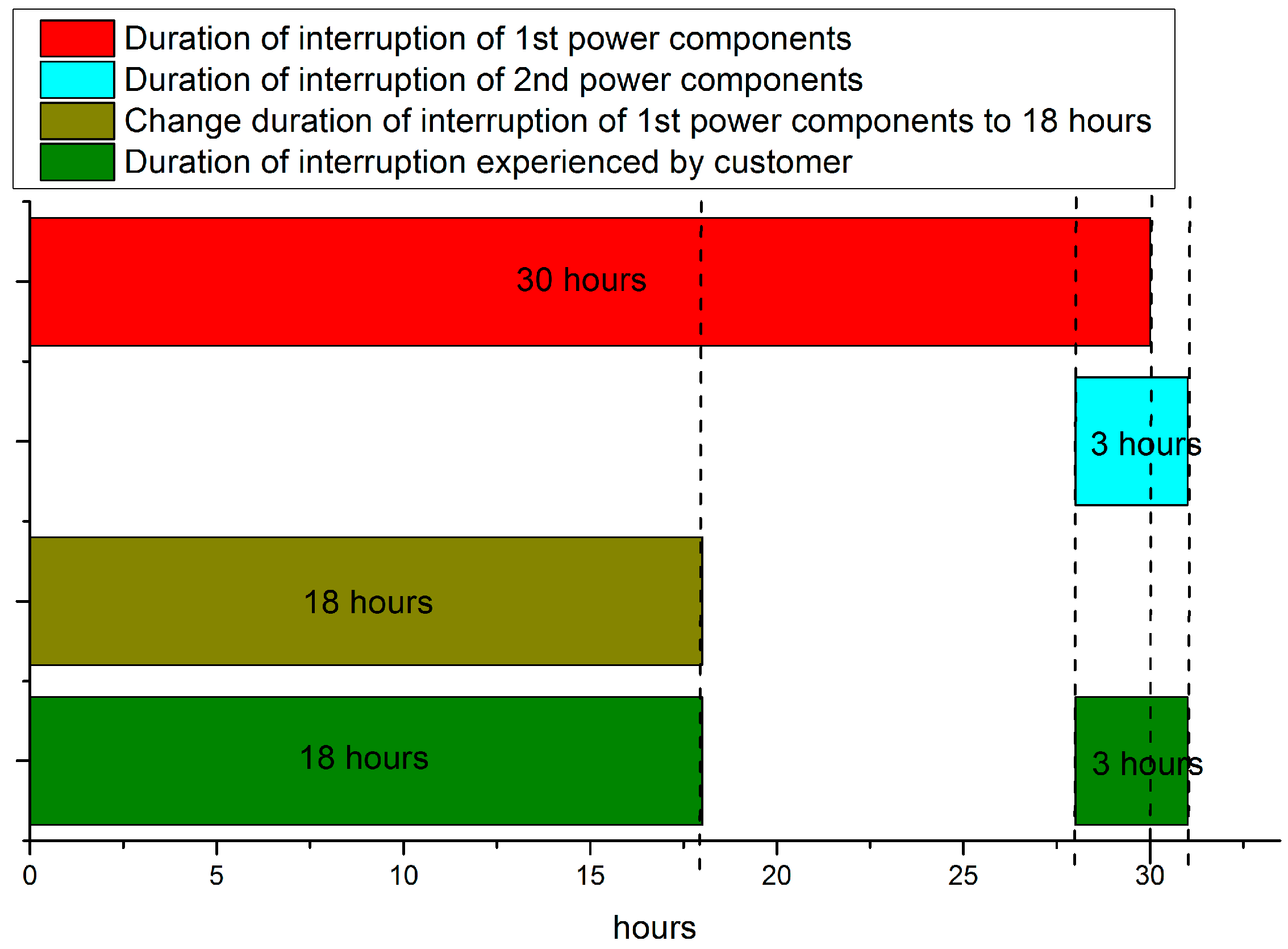
| Scenario SC-4: All LIs (including transfer to alternative supplies and reconfiguration) up to maximum 3 h |
| SC-4A: Reconfiguration at random hours up to 3 h |
| SC-4B: Reconfiguration at exactly 3 h |
| Scenario SC-5: Time for transfer to alternative supply and reconfiguration are exactly 3 min |
| Scenario | Indices | Probabilistic (Mean Values) |
|---|---|---|
| SC-1 | SAIFI | 0.4929 |
| MAIFI | 0.5527 | |
| SAIDI | 33.7625 | |
| CAIDI | 68.4914 | |
| ENS | 3539.4823 | |
| SC-2A | SAIFI | 0.4787 |
| MAIFI | 0.5481 | |
| SAIDI | 6.5735 | |
| CAIDI | 13.7321 | |
| ENS | 669.5330 | |
| SC-2B | SAIFI | 0.4682 |
| MAIFI | 0.5580 | |
| SAIDI | 8.4968 | |
| CAIDI | 18.1494 | |
| ENS | 842.8723 | |
| SC-3A | SAIFI | 0.4847 |
| MAIFI | 0.5597 | |
| SAIDI | 6.1732 | |
| CAIDI | 12.7374 | |
| ENS | 625.1351 | |
| SC-3B | SAIFI | 0.4854 |
| MAIFI | 0.5581 | |
| SAIDI | 8.1339 | |
| CAIDI | 17.6588 | |
| ENS | 831.2357 | |
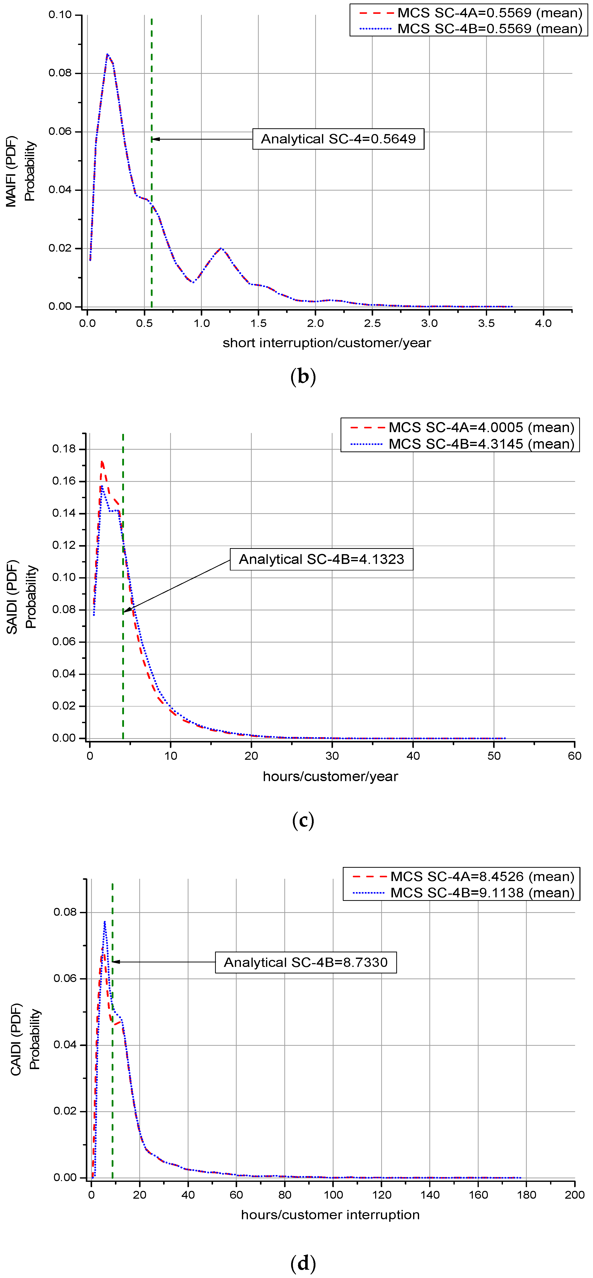
| SC-4A | SAIFI | 0.4733 |
| MAIFI | 0.5569 | |
| SAIDI | 4.0005 | |
| CAIDI | 8.4526 | |
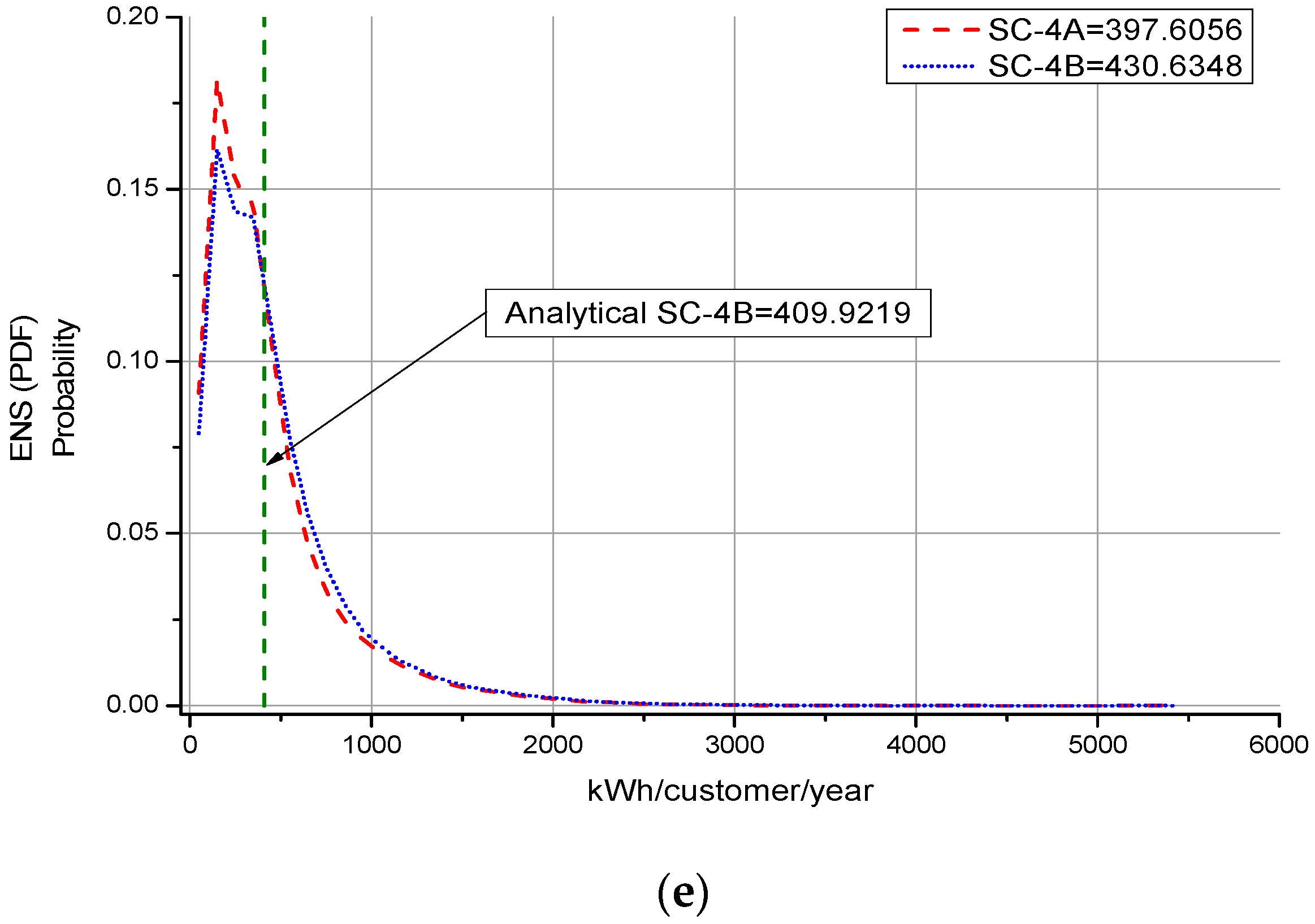
| ENS | 397.6056 | |
| SC-4B | SAIFI | 0.4734 |
| MAIFI | 0.5569 | |
| SAIDI | 4.3145 | |
| CAIDI | 9.1138 | |
| ENS | 430.6348 | |
| SC-5 | SAIFI | 0.1514 |
| MAIFI | 0.8785 | |
| SAIDI | 3.3554 | |
| CAIDI | 22.1576 | |
| ENS | 346.5313 |
© 2019 by the authors. Licensee MDPI, Basel, Switzerland. This article is an open access article distributed under the terms and conditions of the Creative Commons Attribution (CC BY) license (http://creativecommons.org/licenses/by/4.0/).
Share and Cite
Muhammad Ridzuan, M.I.; Djokic, S.Z. Energy Regulator Supply Restoration Time. Energies 2019, 12, 1051. https://doi.org/10.3390/en12061051
Muhammad Ridzuan MI, Djokic SZ. Energy Regulator Supply Restoration Time. Energies. 2019; 12(6):1051. https://doi.org/10.3390/en12061051
Chicago/Turabian StyleMuhammad Ridzuan, Mohd Ikhwan, and Sasa Z. Djokic. 2019. "Energy Regulator Supply Restoration Time" Energies 12, no. 6: 1051. https://doi.org/10.3390/en12061051
APA StyleMuhammad Ridzuan, M. I., & Djokic, S. Z. (2019). Energy Regulator Supply Restoration Time. Energies, 12(6), 1051. https://doi.org/10.3390/en12061051