Flow Conditions for PATs Operating in Parallel: Experimental and Numerical Analyses


1
Department of Civil Engineering, Architecture and Georesources (DECivil) and CEris member, Instituto Superior Técnico, University of Lisbon, 1049-001 Lisboa, Portugal
2
Hydraulic and Environmental Engineering Department, Universitat Politècnica de València, 46022 Valencia, Spain
3
Department of Hydraulic, Geotechnical and Environmental Engineering, Università di Napoli Federico II, via Claudio, 21, Napoli 80125, Italy
*
Author to whom correspondence should be addressed.
Energies 2019, 12(5), 901; https://doi.org/10.3390/en12050901
Submission received: 24 January 2019
/
Revised: 21 February 2019
/
Accepted: 5 March 2019
/
Published: 8 March 2019
(This article belongs to the Special Issue Electrical Energy Production in the Water Sector)
Abstract
:Micro-hydro systems can be used as a promising new source of renewable energy generation, requiring a low investment cost of hydraulic, mechanical, and electrical equipment. The improvement of the water management associated with the use of pumps working as turbines (PATs) is a real advantage when the availability of these machines is considered for a wide range of flow rates and heads. Parallel turbomachines can be used to optimize the flow management of the system. In the present study, experimental tests were performed in two equal PATs working in parallel and in single mode. These results were used to calibrate and validate the numerical simulations. The analysis of pressure variation and head losses was evaluated during steady state conditions using different numerical models (1D and 3D). From the 1D model, the installation curve of the system was able to be defined and used to calculate the operating point of the two PATs running in parallel. As for the computational fluid dynamics (CFD) model, intensive analysis was carried out to predict the PATs′ behavior under different flow conditions and to evaluate the different head losses detected within the impellers. The results show system performance differences between two units running in parallel against a single unit, providing a greater operational flow range. The performance in parallel design conditions show a peak efficiency with less shock losses within the impeller. Furthermore, by combining multiple PATs in parallel arrangement, a site’s efficiency increases, covering a wide range of applications from the minimum to the maximum flow rate. The simulated flow rates were in good agreement with the measured data, presenting an average error of 10%.
1. Introduction
Hydropower is a renewable energy source, is non-polluting, with low operational costs, and is environmentally friendly compared to other sources of energy [1,2]. Considered as a promising solution to provide energy in micro or large scales, hydropower is the most renewable energy produced accounting for 90% of the total worldwide renewable energy [3]. Micro-hydropower schemes can provide a new solution for the energy scarcity mostly detected in rural and isolated areas, where the extension of the electric grid is techno-economically unfeasible [2,4].
Micro-hydro systems must have optimal components selection and operation to minimize the overall costs. The application of a pump as turbine (PAT) instead of a conventional turbine is an alternative solution due to its easy implementation and reduced investment costs [5]. The advantages of pumps, in turbine mode, over conventional hydro turbines are: cost effective, less complex, available for a wide range of applications with short delivery time, and feasible [6,7]. Thus, the use of a PAT for micro-hydropower offers a low-cost solution as compared to a conventional micro-hydro turbine.
In recent years, the possibility of using PATs is an attractive solution for simultaneously controlling pressure and the energy generation and improving the sustainability and management of water systems [8,9,10,11,12]. Mostly, pumps work as turbines, in the range 1–500 kW, with 5–15 m and 50–150 L/s for head and flow rates, respectively. For heads ranging from 15 to 100 m and flow rates ranging from 50 to 1000 L/s, double suction pumps or multi centrifugal pumps in a parallel arrangement, are suitable [13]. The introduction of the PATs in water systems demonstrated the need to use different machines in parallel to reach all flow range along line [11]. Several studies proposed parallel use, but none combined experimental and analytical analyses to describe this configuration [10].
PATs can be planned to take into account the minimum flow rate running in parallel to achieve a better performance considering the system’s flow variations, which in water pipe systems are commonly dependent on the variable demand pattern. When examining or designing a PAT system, the process demands must first be established and the most energy efficient solution included. Variation of flow rate is achieved by switching on and off additional PATs to meet demand. The combined PAT curve is obtained by adding the flow rates at a specific head. The efficiency response provides an essential cost advantage; by keeping the operating efficiency as high as possible across variations in the system’s flow demand, the energy and maintenance costs of the PAT can be significantly reduced. If two or more PATs are operating in parallel, they can be switched on/off according to the available flow [12]. In this situation, the flow rate and pressure requirements for an optimal energy production can be managed using multiple PATs in reverse mode [13]. Moreover, running PATs in parallel requires a suitable control, to operate near the best efficiency point (BEP) conditions as possible being an advantage over a single turbine [8,14,15]. Hence, detailed investigation is required before deciding the number of PATs.
In this research, two PATs running in parallel and in a single mode were examined experimentally and numerically, using hydraulic solvers and computational fluid dynamics (CFD) models. Different inlet flow rates were tested for two configurations: one single PAT working and two PATS running in parallel. A 1D model was used to define the installation curve of the system, where two general purpose valves (GPV) were used to define the PATs. Several scenarios were simulated in order to study pressure fluctuations, losses distribution, and net head availability in each layout. Head losses can be estimated in an easy way in pipes, valves, elbows, among others singularities, but they are still not known in PATs, in particular during parallel operation. Thus, the main focus of this research is to know not only the variation of the best efficiency when PATs are installed in parallel and their influence in the improvement of the flow water management in real case studies, but also to evaluate the head losses distribution during reverse mode.
2. Head Losses within PATs
When the machine operates in reverse mode, the pattern of loss distribution differs from the pump mode as a consequence of the reverse flow. Hence, to account the performance and behavior of PATs, one of the utmost factors is the identification of the incurred losses. According to [10,16,17,18], the relationship between pumps and turbines depends on: (i) the flow pattern, due to the specific speed of each machine, and (ii) losses that are related to leaks and frictions. When the fluid passes through the impeller, it is under non-uniform velocity distribution friction effects, flow separation, shear stress, and leakage losses during pump and turbine modes. However, the magnitude of these losses is not the same, since the energy transfer from the rotating impeller to the fluid or vice-versa is not achieved in the same way for pump or turbine modes since the machine was designed to operate as a pump. When a PAT operates at optimum flow conditions, pressure and flow direction act on the impeller resulting in shock and friction losses [14,19], which can be classified as internal losses due to fluid friction in the stationary and rotating blade passage.
The flow within the impeller and in the draft tube is decelerating. Therefore, the frictional losses are related to skin friction and boundary layer separation that depend on the friction factor length of the flow passage and the turbulent fluid velocity [16,20,21]. Also, a certain leakage of fluid from the high pressure side of the machine to the low pressure side through the small passages between the impeller and the casing can be noticed, leading to a waste flow energy [14,22]. The leakage losses comprise a small fraction of the total loss. In addition, a small part of the fluid passing through the leaks around the impeller does not contribute to the energy transfer [2].
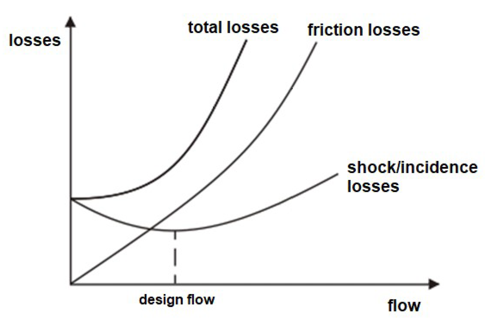
During the off-design conditions, the direction of the relative velocity of fluid at the impeller inlet does not match with the inlet blade angle, due to the lack of a guide vane. As a result, the fluid flow cannot enter the blade passage smoothly by sliding along the blade surface [16,20]. These losses of energy are known as incidence or shock losses, as shown in Figure 1 Shock losses usually occur at low velocities and reach the minimum value at the designed flow rate [20,23,24]. Therefore, the total losses can be defined by Equation (1):
where are the total losses in PAT (m.wc.); are the friction losses inside of impeller (mw.c.); and are the incidence losses of the flow inside of the impeller (mw.c.).
In fact, the shock losses should be zero, at the designed flow rate. However, as shown in Figure 1, incidence losses comprise both shock losses and impeller entry losses due to a change in the direction of the flow from a radial to axial direction, in the vaneless space (i.e., gap), before acting in the blades. The impeller entry losses are similar to a pipe bend and are very small compared to other losses [19,22]. Thus, the incidence losses show a non-zero minimum value at the designed flow rate.
When passing from an increased flow rate in a convergence passage (i.e., during turbine mode) to a divergence way (i.e., in pump mode), the friction losses increase [14], as well as the leakages and vorticities, due to a pressure variation. Thus, shock losses have an important role in a PAT behavior, in particular when associated with smaller rotational speeds [14,25,26,27].
3. Experimental Set-Up
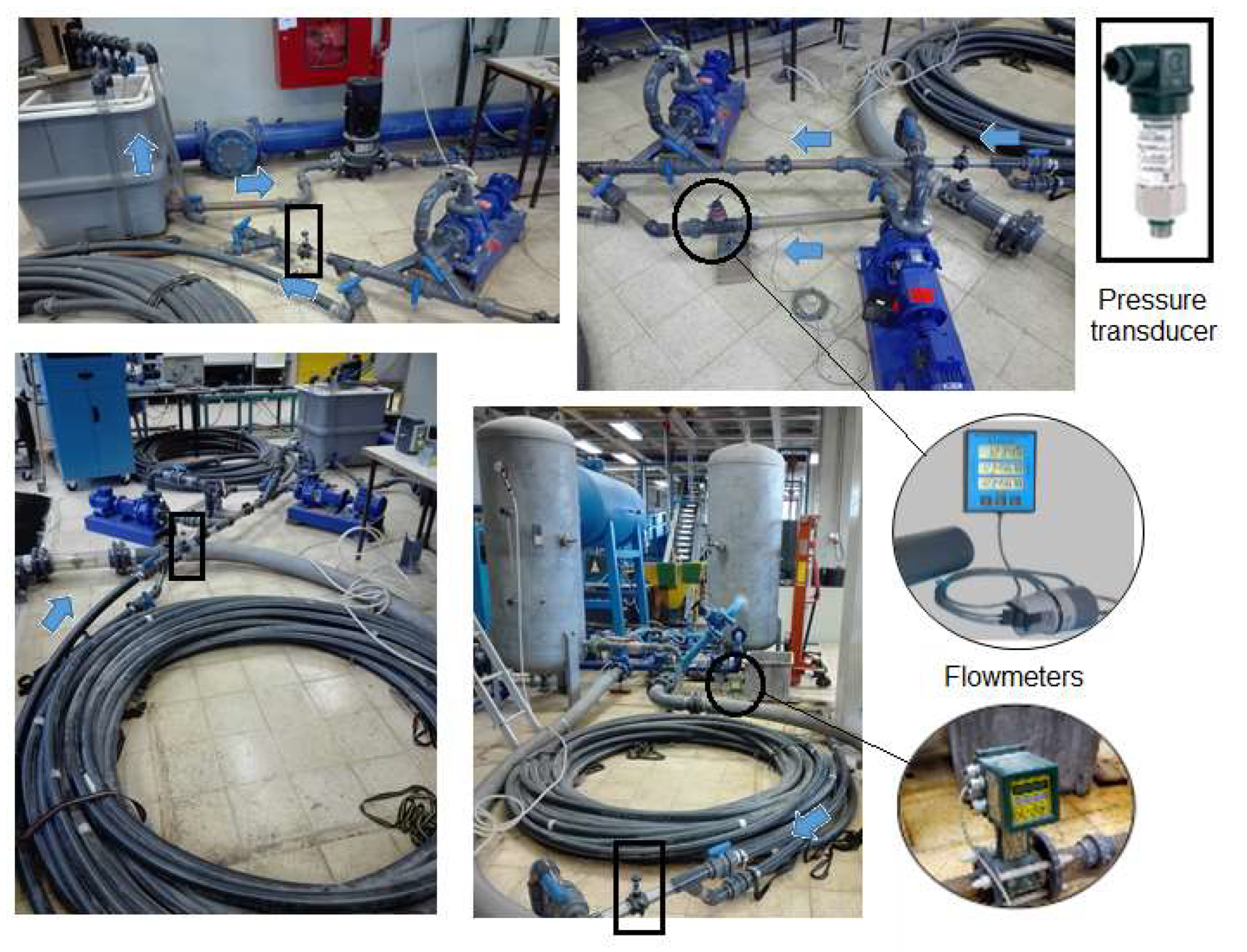
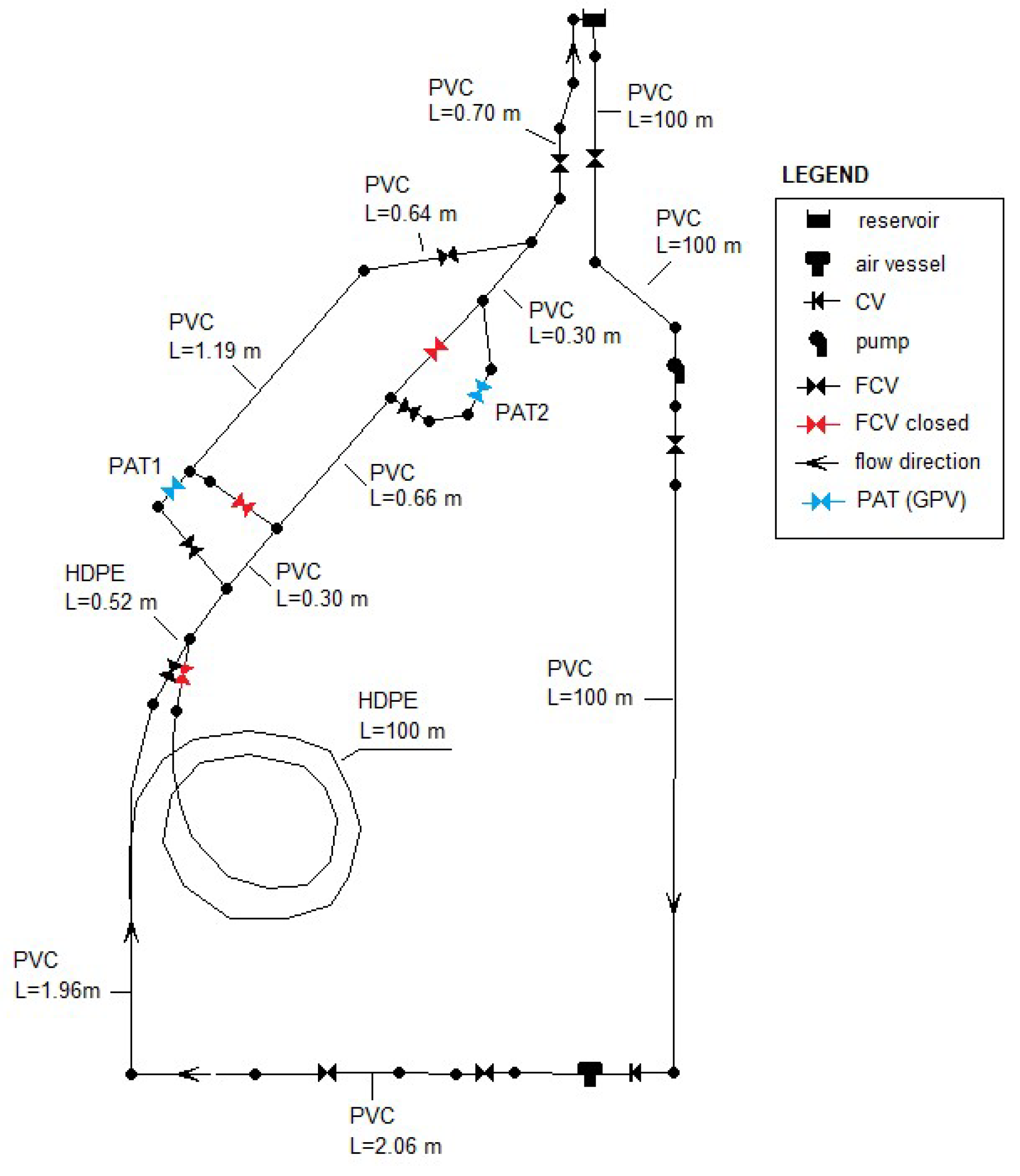
Figure 2 shows the scheme and photos where several experimental tests were conducted on two parallel PATs (Etanorm 32-125 from KSB) at the Hydraulic Laboratory in the Department of Civil Engineering, Instituto Superior Técnico, Universidade de Lisboa. The experimental facility was composed of polyethylene and PVC pipes with a nominal diameter (ND) of 50 mm, regulated by an air vessel, with a maximum pressure of 125 m. Ball valves were installed along the system, for flow control and regulation. Two pressure transducers and a flowmeter were also deployed in the system to characterize different parameters at specific significant points, such as two electromagnetic flowmeters located downstream of the air vessel and downstream of PAT1, as shown in Figure 2, respectively. The pressure transducers, installed upstream and downstream of the PATs, present a pressure range of 0 to 10 bar with an accuracy of 0.25%.
Several experimental tests were carried out twirling the PATs at different rotational speeds starting from 200 to 1150 rpm, for the two configurations (two PATs in parallel and a single PAT) by regulating the flow rate. During each test, the data were recorded (i.e., the discharge Q, net head h, and rotational speed N). Table 1 shows the test results and the PATs’ range application.
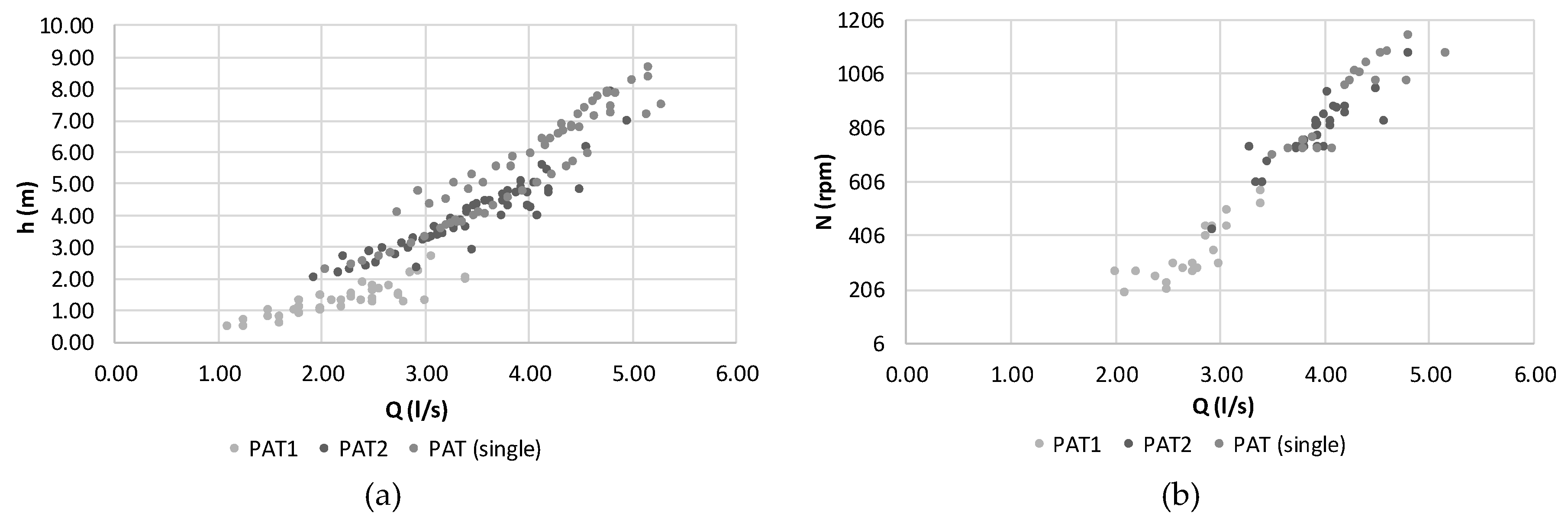
Figure 3 presents the PATs’ curves, in each machine, working in single and in parallel modes. Data exhibited different values for each PAT during the parallel tests, since the impellers run at different speeds and consequently different flow rates. Due to the lab pipe system non-symmetric layout for two PATs in parallel, different flow rates and head to each PAT, the total that passes through PAT1 (upstream) is around 22% less than at PAT2 (downstream), allowing a better flow adaptation to the water system demand (with low flows at right and higher values during the rush hours).
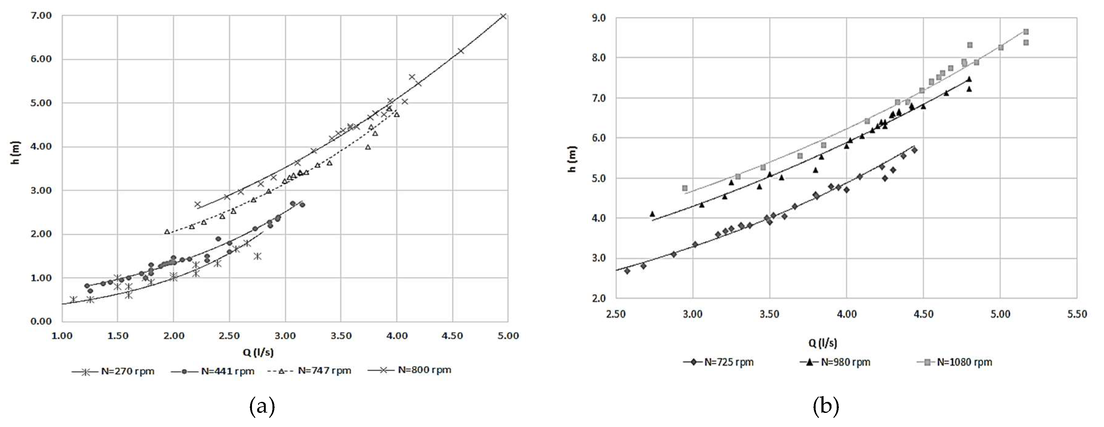
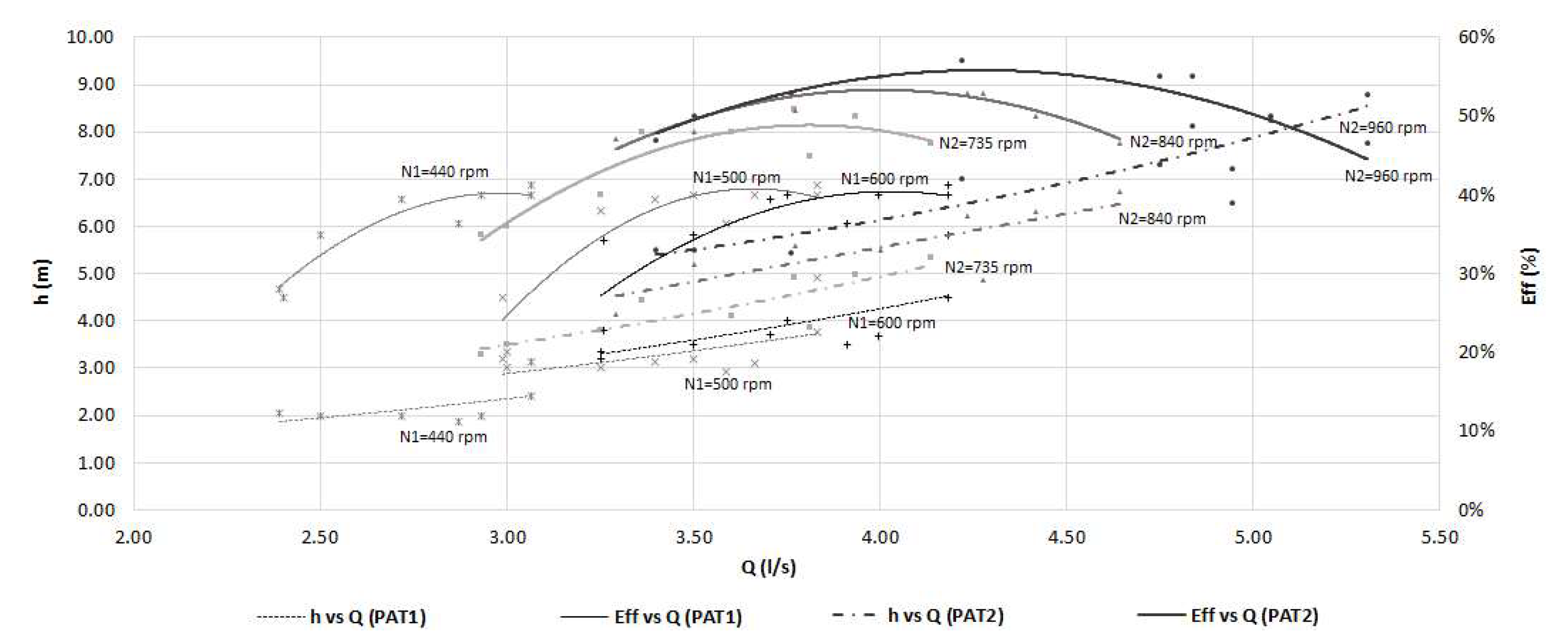
Figure 4a presents the characteristic curves (CC) of the PATs for different rotational speeds (i.e., 270–441 rpm for PAT1 and 735–800 rpm for PAT2) when the machines operate in parallel in a non-symmetric configuration. Figure 4b also shows PATs operating in single mode (i.e., 725–1080 rpm), identifying the rotational speed in each PAT configuration.
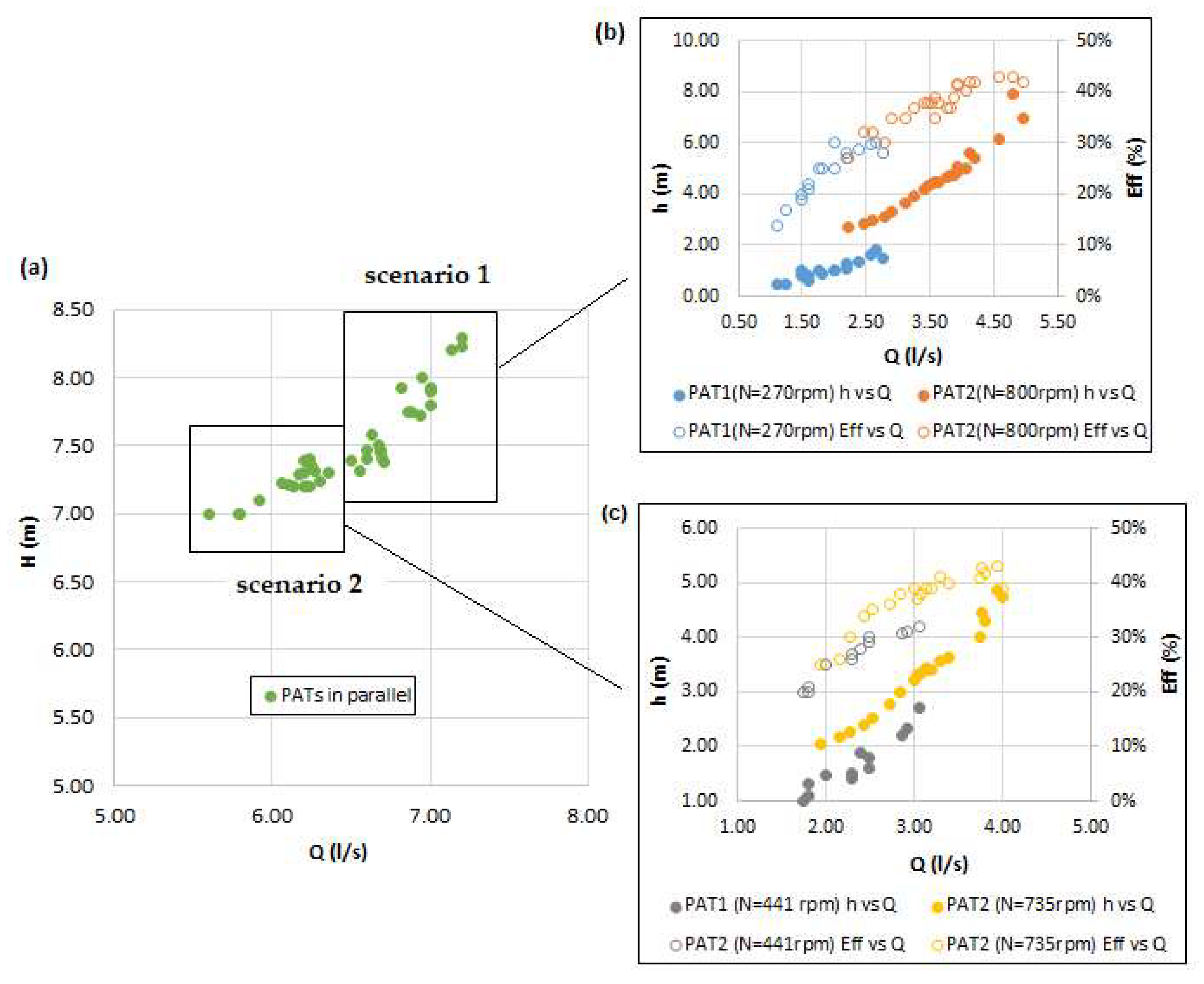
Figure 5a shows two flow combinations between 5.80 and 7.20 L/s in parallel mode. In scenario 1, until a total flow of 6.60 L/s, PAT1 rotated at 270 rpm (i.e., 2.40 < Q < 2.87 L/s) against 800 rpm for PAT2 (i.e., 2.90 < Q < 3.95 L/s), as shown in Figure 5b. As for scenario 2, at higher than 6.60 L/s, PAT 1 and PAT2 rotated at 441 rpm (2.4 L/s < Q < 3.0 L/s) and 735 rpm (3.77 L/s < Q < 4.81 L/s), respectively, as shown in Figure 5c.
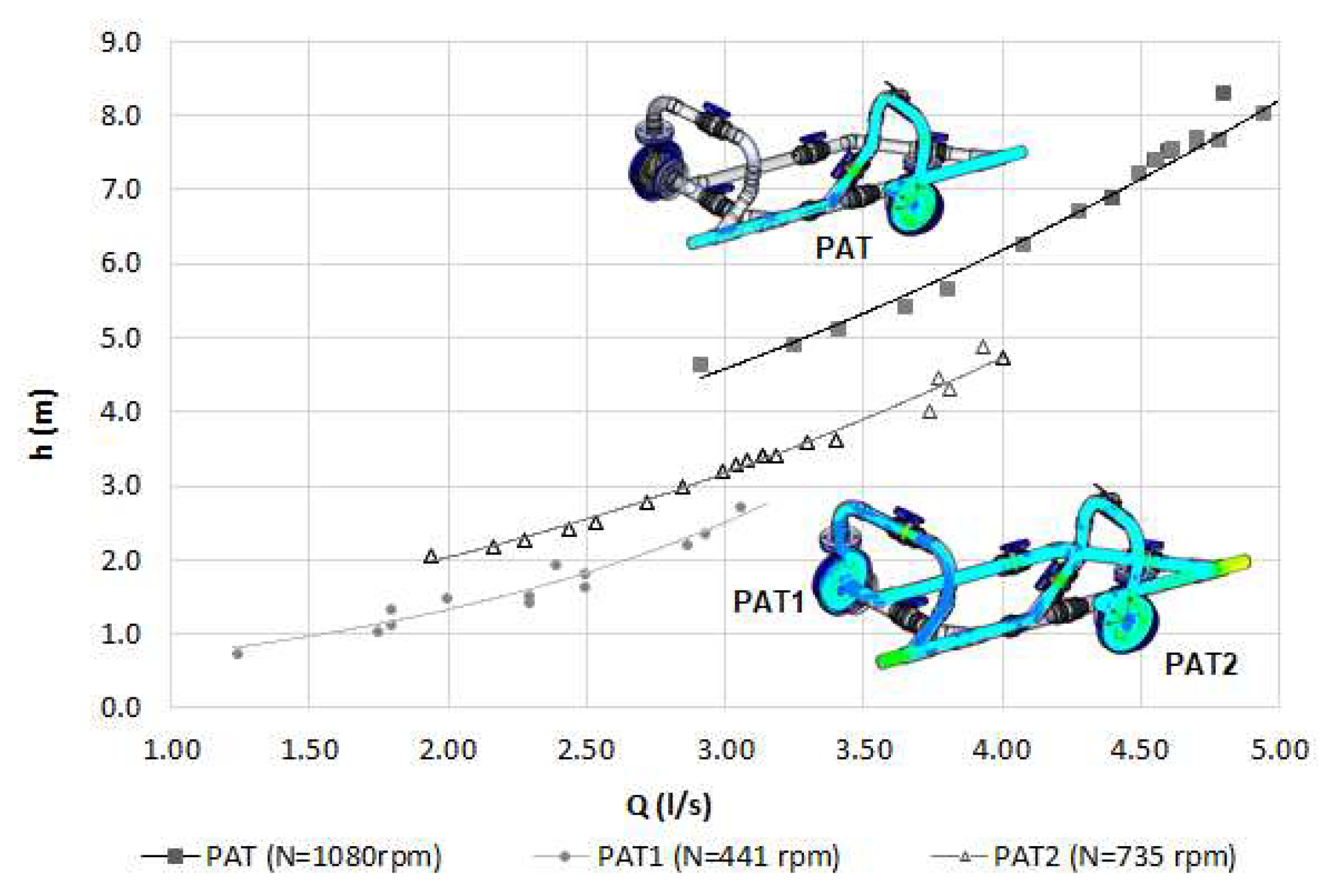
Figure 6 shows the single PAT attaining the rotational speed N = 1080 rpm. The fraction of the flow by both PATs induces consequent reductions on the flow and rotational speed of each PAT in parallel. The experimental tests were used in the CFD model for calibration and validation.
4. Numerical Simulations
4.1. EPANET Model
The experimental set-up was modelled in EPANET [15] which is a hydraulic solver model from EPA-US that uses a visual interface to model pressurized systems. EPANET calculates the hydraulic head and pressure at every node; the flow rate, the flow velocity, and the head loss in each pipe branch and the hydraulic head in each tank or air vessel. The water system of the experimental set-up was built with the following elements: 1 tank, 1 pump, 10 open flow control valves (FCV), 2 closed FCV, 2 PATs, 1 check valve (CV), and 1 air-vessel. Since EPANET does not have a predefined turbine object as a network element, the 2 PATs were simulated using GPV, defining the flow-head loss curve correspondent to the PATs’ characteristic curves, as shown in Figure 7.
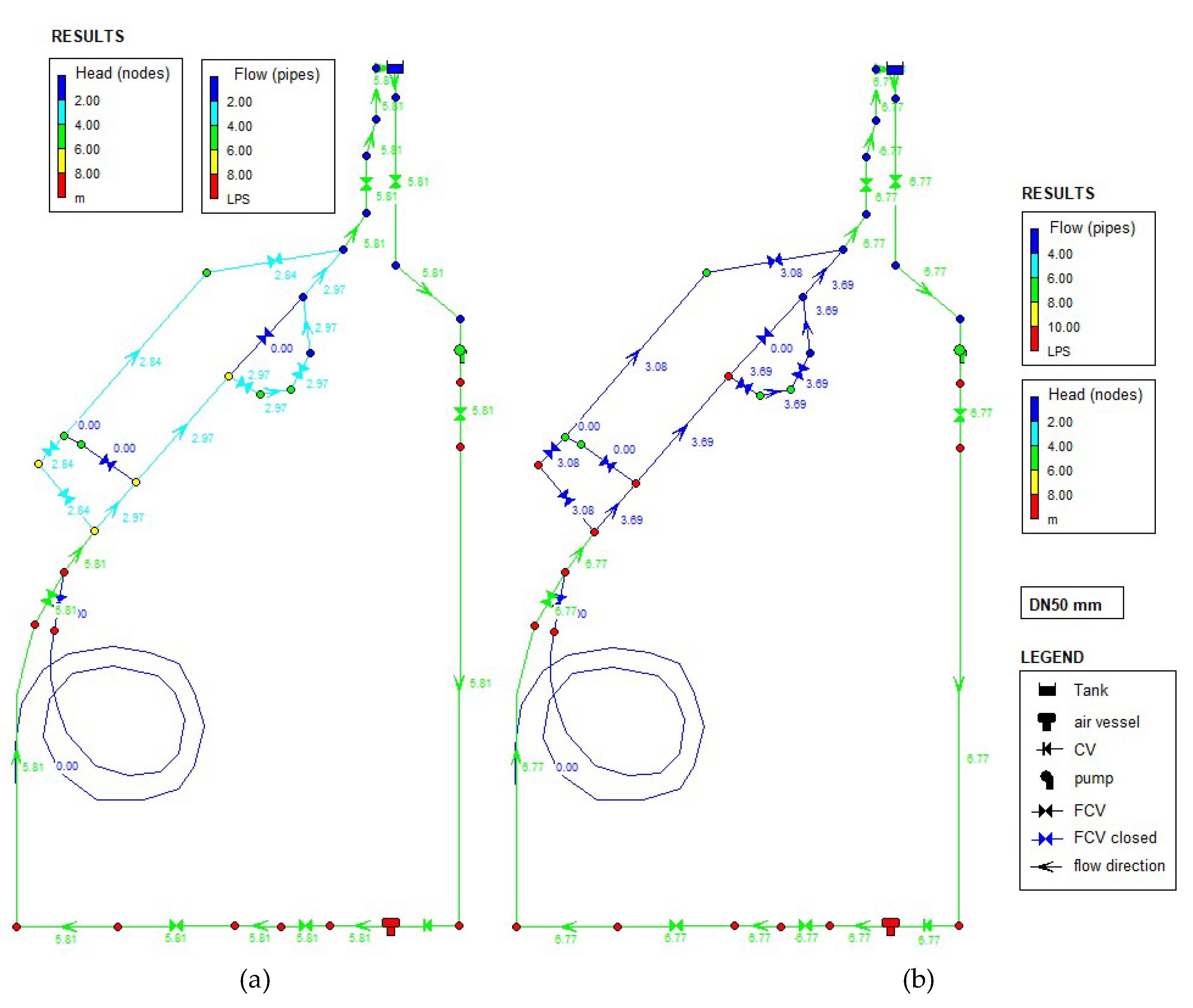
The time for the simulation was set to 5 h with a time step of 0.2 h (12 min). The network was calibrated, as shown in Figure 8, considering the characteristic curves of the PATs, as shown in Figure 4, both single and parallel operation, the inlet and outlet pressure in the air-vessel, and the water level in the tank.
The results show, for two of the tested scenarios with the corresponding CC of the PATs (from Figure 4), reliable values with correlation factors above 0.98 between 1D and experimental tests. This model allows for the obtaining of the system curve of the network for different values of operating flow.
4.2. CFD Model
4.2.1. PAT Geometry and Mesh
Computational fluid dynamics (CFD) is an effective tool for predicting the performance of PATs, identifying losses in hydraulic machine components, such as in the volute, impeller, draft tube, bends, and valves, and in the designing and performance analysis of fluid dynamics inside turbo machines [24]. These tools allow modelers to simulate the hydraulic flow in virtual conditions, due to the advances in numerical algorithms and computing power. Several parameters can be investigated using CFD models (e.g., flow separation zones, vorticity, paths inside the impeller, cavitation analysis, loss distribution, shear stress), which are very difficult to perform and visualize by experimental tests. The calibration of these models enables the extrapolation of the analysis to other flow conditions. Also, CFD can provide a pinpoint insight of local flow phenomena and pressure fluctuations along the pipe network [1]. One of the major benefits of calibrated CFD models is that it does not require development of complex physical models, being quite pertinent in particular in complex hydro mechanical devices with interaction of different components, or shapes and operating modes [28].
The most time consuming stages during the calibration process is related to the mesh definition. Thus, it is necessary to find a balance between a high mesh resolution for suitable accuracy and a low mesh resolution in order to reduce the computational time under particular computer specifications [20]. This process can be optimized until reaching a reasonable cpu time without impairing the accuracy. This reduction of cpu time is crucial for the calibration procedure, since several scenarios need to be tested and may take several hours to be completed, plus the time for analyses and modifications.
The PATs’ system was built in SolidWorks—FloEFD model. The governing equations were discretized and solved using the finite volume method (FVM) on a spatial rectangular computational mesh refined locally at the solid/fluid interfaces and in specified fluid regions, where high gradients are expected, according to [20]. FloEFD solves the Navier–Stokes equations and employs the transport equations for the turbulent kinetic energy and its dissipation rate, (i.e., the k-ε model). The conservation laws for mass and momentum in Cartesian coordinate system rotation can be written in the conservation form as [29]:
where, is the fluid density, is the fluid velocity, and is the viscous shear stress tensor. For Newtonian fluids this tensor is expressed as [19]:
Where the Reynolds-stress tensor, following Boussinesq assumption, is [29]:
Herein, is the Kronecker delta function (it is equal to 1 when i = j, and zero otherwise), is the turbulent eddy viscosity coefficient, is the dynamic viscosity coefficient, and is the turbulent kinetic energy. For the k-ε turbulence model, two basic turbulence properties are defined, namely, the turbulent kinetic energy k and the turbulent dissipation ε [16].
where, is a turbulent viscosity factor, with , and y defines the distance to the wall.
A Semi-Implicit Method for Pressure-Linked Equations (SIMPLE) algorithm was used to couple the velocity and pressure [29]. A relative error for the convergence criterion was considered less than 10−4. The rotating components were computed in the Cartesian system attached to the rotating parts, i.e., the stationary parts must be axisymmetric relative to the rotation axis [16].
The generation of the mesh begins with the definition of a rectangular computational domain automatically built, enclosing the solid body with the orthogonal boundary planes to the specified axes of the Cartesian coordinates system, according to [30]. Following [30], the intersection of these planes defines the set of rectangular cells that creates the base mesh. The software crosses the mesh cells sequentially and for each cell, it parses the geometrical configuration inside the cell, followed by a refinement criterion [30]. Hence, for each cell, a refinement value is calculated individually according to an algorithm that controls the type of refinement. Setting refinement levels individually for each criterion makes it possible to influence the total number of generated cells. The refinement level is the number of times that is refined relative to the initial cell in the base mesh [20].
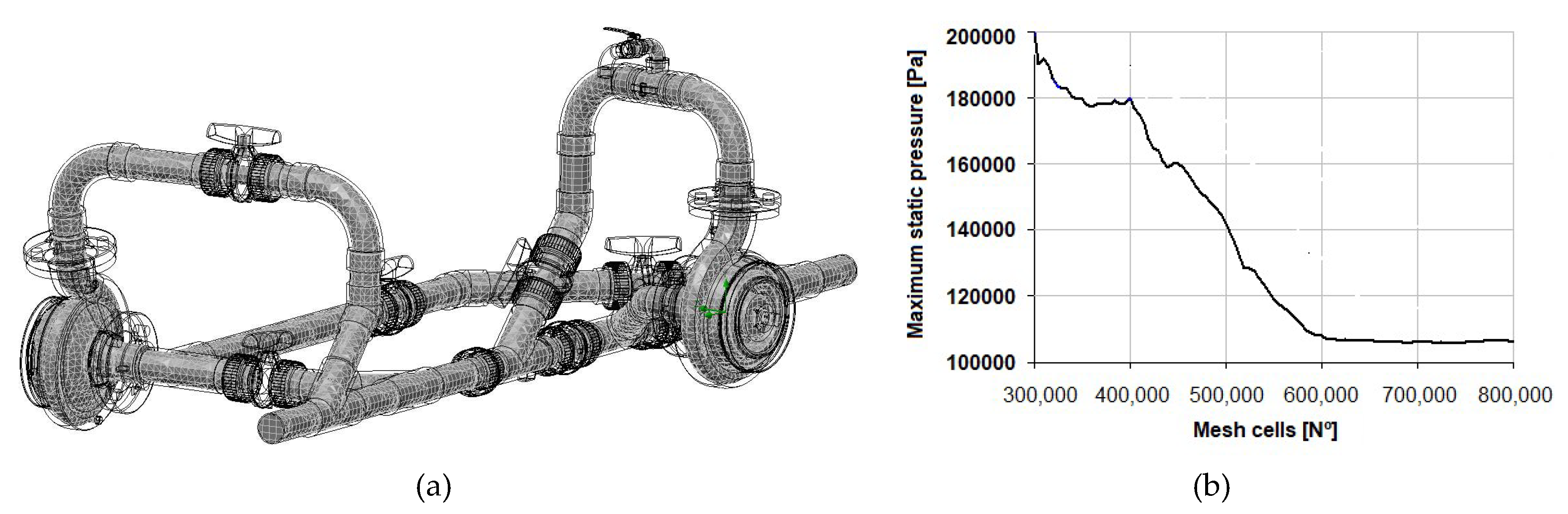
Thus, the mesh is refined such that the solution is left to be dependent on the mesh size. By ensuring that there is no mesh space dependency, a mesh sensitivity analysis is conducted by triggering the solution-adaptive meshing. This allows to increase automatically the number of cells in areas with high flow gradient while still maintaining the flow solution [20]. The mesh was performed by starting with an initial coarse mesh with 85,832 cells, followed by a mesh refinement process. The process was stopped when the difference in the maximum static pressure for a specific point of the domain, between consecutive meshes was less than 2%, which occurred for 713,954 cells, as shown in Figure 9.
4.2.2. Boundary Conditions
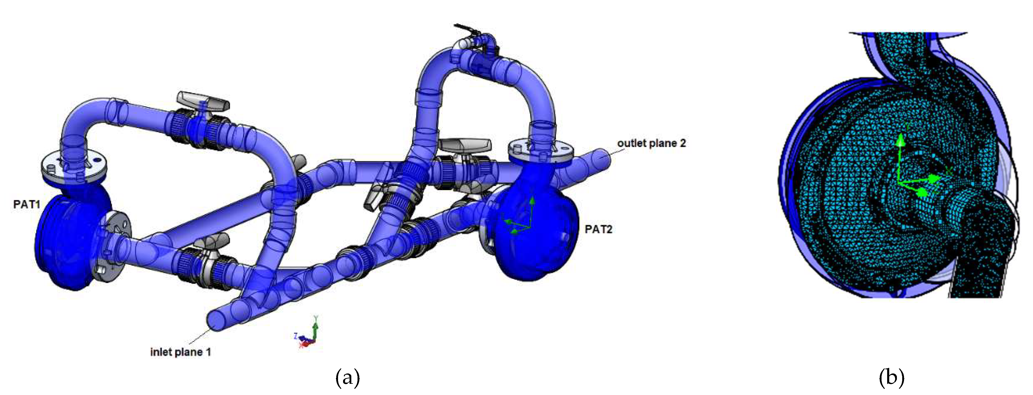
The simulations were carried out at the identical load points from the experimental study. The variables, such as mass flow rate, outlet pressure, and rotational speed, were transferred from experimental measurements. The mass flow rate used in the numerical model was the discharge across the PAT system without any leakage. The boundary conditions comprised the flow rate at the inlet plane 1, as shown in Figure 10a, the constant static pressure at the outlet plane 2, and the rotational speed set for each impeller. The standard k-ε was used together with a standard wall function. The wall interface was set to a no-slip condition over the wetted surface.
In the CFD model, it was necessary to specify the rotating zones used to analyze the flow within the impeller. The rotating solid component, surrounded by an axisymmetric rotating zone and the fluid flow equations in the non-rotating zones (stationary) of the computational domain, were solved in the non-rotating Cartesian global coordinate system [29]. Thus, the influence of the rotation’s effect on the flow was taken into account in the equations written in each of the rotating coordinate systems. Internal boundary conditions were set at the fluid boundaries of the rotating zones, to connect solutions obtained within the rotating zones and in the non-rotating part of the computational domain [29]. Consequentially, to correctly set these boundary conditions and the rotating coordinate system, a rotating region was specified [16].
5. Results and Discussion
5.1. Pressure Variation and Velocity Streamlines Distribution
Numerical simulations were developed for the two PATs operating in parallel and in a single mode, as shown in Figure 11. As switching from single mode to parallel, lower rotational speed curves are concentrated towards the bottom left in Figure 11 and for subsequent higher rotational speeds the h-Q-η curves move towards the top right in Figure 11. The individual PAT presented different values of efficiency, which depended on the hydraulic condition under each steady state regime.
Simulation and experimental results showed the PAT flow rate of 3.80 L/s at the BEP (working in a single mode). In parallel mode, the rotational speed in each PAT was different, influencing the h-Q-η curves, respectively, in PAT1 and PAT2, as shown in Figure 11. Both PATs display different rotational speeds covering a wide range of discharge values when working in parallel.
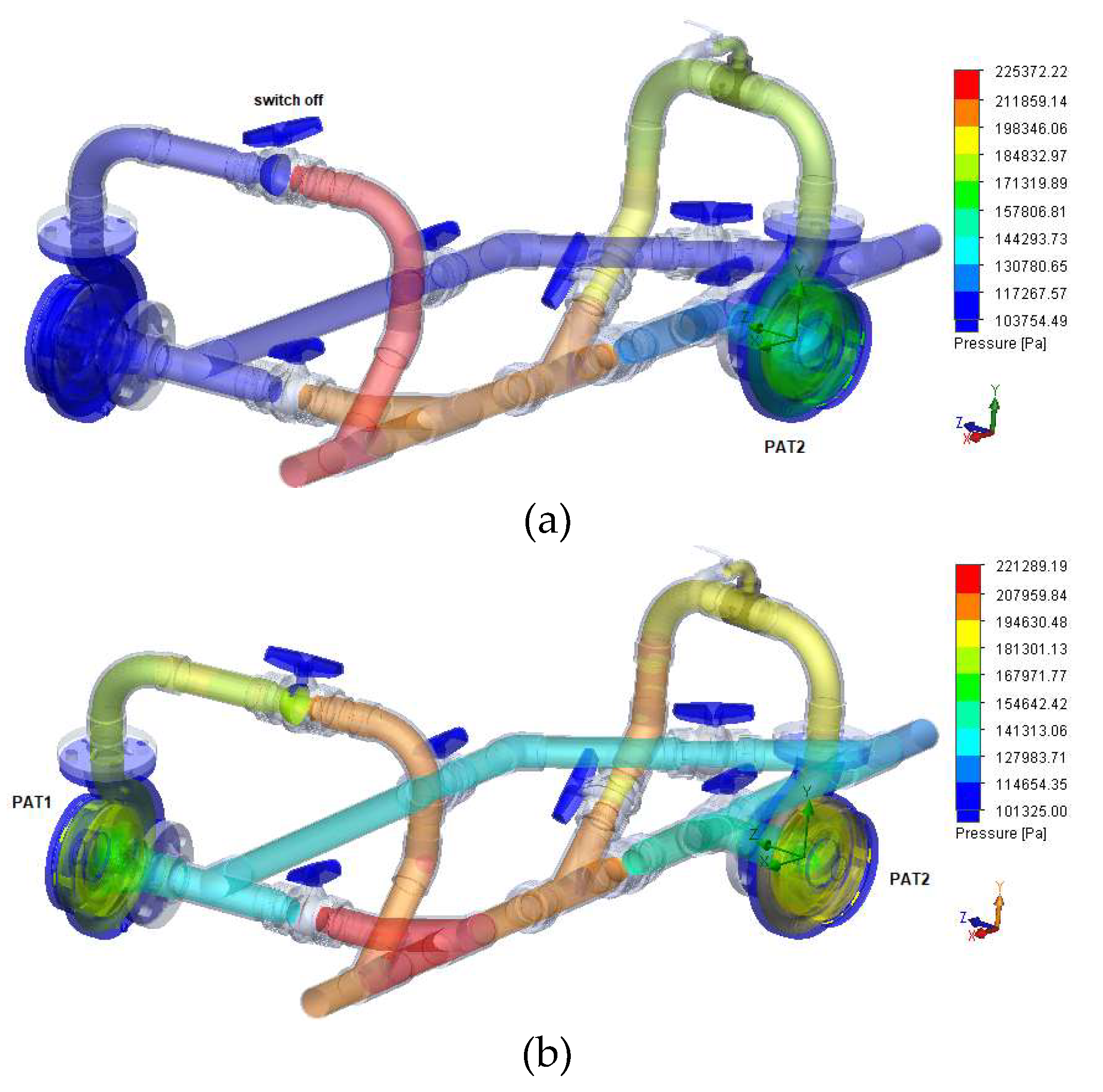
Figure 12a shows the pressure variation, of the single PAT2, at BEP condition. Overall, in Figure 10b, the simulation analysis concluded lower flow values and rotational speeds during parallel PATs operation, due to the designed non-symmetric configuration.
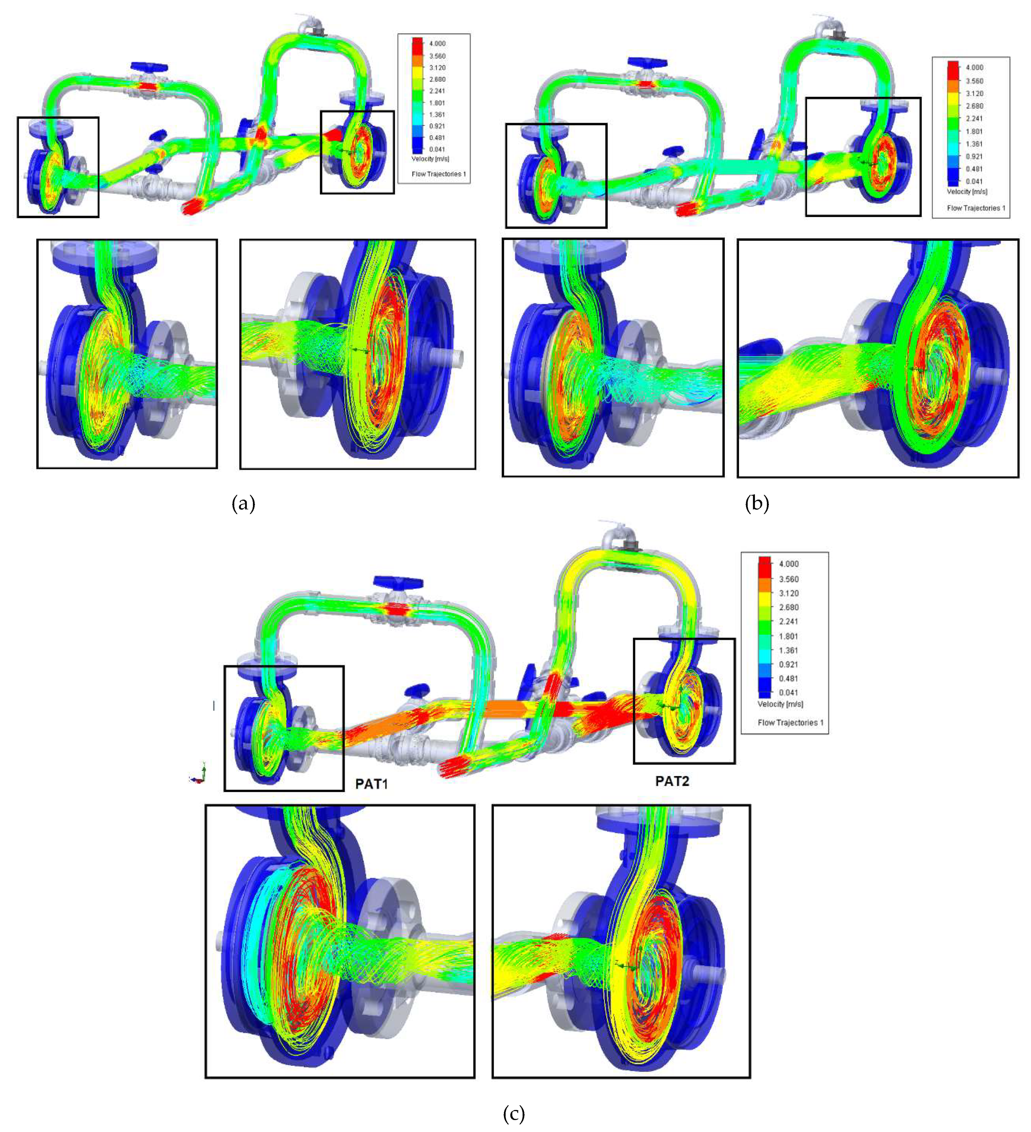
Figure 13 shows the velocity streamlines distribution, specifically the rotation of the flow through the two impellers and along the draft tube. The flow near the impeller varies with the rotational speed, inducing different behaviors: low velocity values in the vortex core (i.e., near the axis of the draft tube) that was formed downstream of the runner, and the remarkable velocity streamlines that reach the wall of the draft tube due to the flow rotation, visible in Figure 13c.
The rotational behavior was also verified as well as the centrifugal force that arose with the increase of the impeller rotation. The flow entered the volute and exerted a radial force on the impeller, thereby imparting a rotational speed to the rotor [25]. Consequently, as the speed ratio increased, a high concentration of velocity streamlines migrated from the outside to the core side of the runner. Hence, with the rotational speed increasing, additional vibrations, turbulences, and consequently, dissipative effects, arose [17,18,24,31,32].
5.2. Analysis of the Head Losses of the PATs System
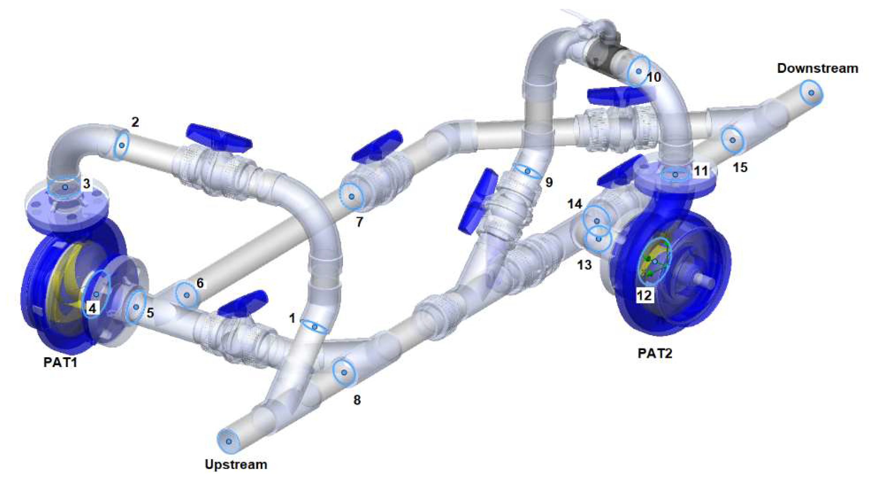
In the CFD model, numerical simulations were carried out to determine the losses, in different components for different inlet conditions. Monitor points were defined, in the computational domain, by dividing the system according to Figure 14. The regions of losses were identified as 1 and 9 in the inlet derivations, for the respective PATs, immediately upstream of the inlet curve (points 2 and 10), upstream of the casing (points 3 and 11), in the rotating impeller (points 4 and 12), in the draft tube (points 5, 6, 13 and 14), and downstream of the draft tube (points 7 and 15).
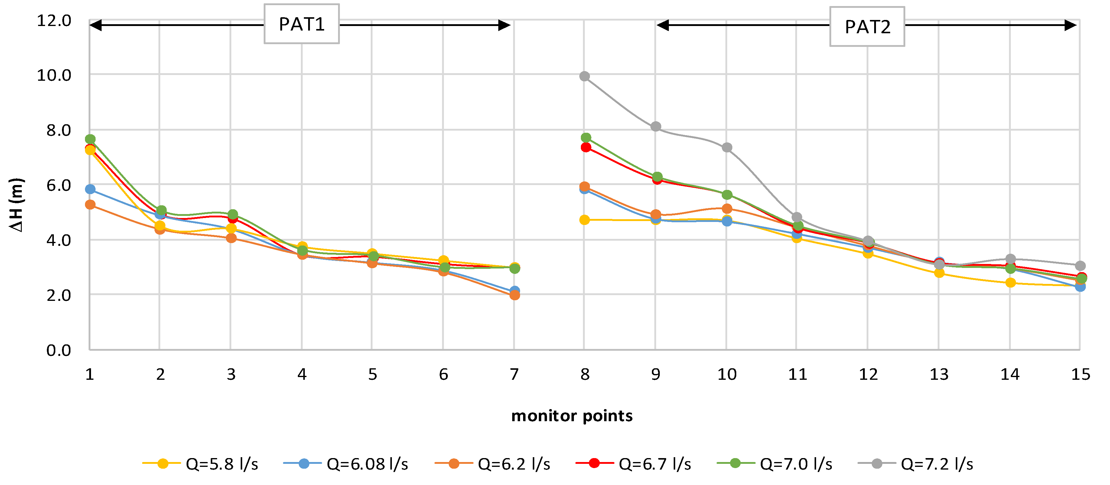
Figure 15 shows the internal losses distribution in the control volume at different flow rates, in parallel mode, obtained from CFD simulations. Losses until the volute casing (before points 3 and 11) show increasing losses with the flow in inlet pipes. After that, the losses of the impeller zone (points 4 and 12, points 5‒7, and 13‒15) were concentrated points of rotating flow almost independent of the flow. The draft tube losses were associated to the swirl flow.
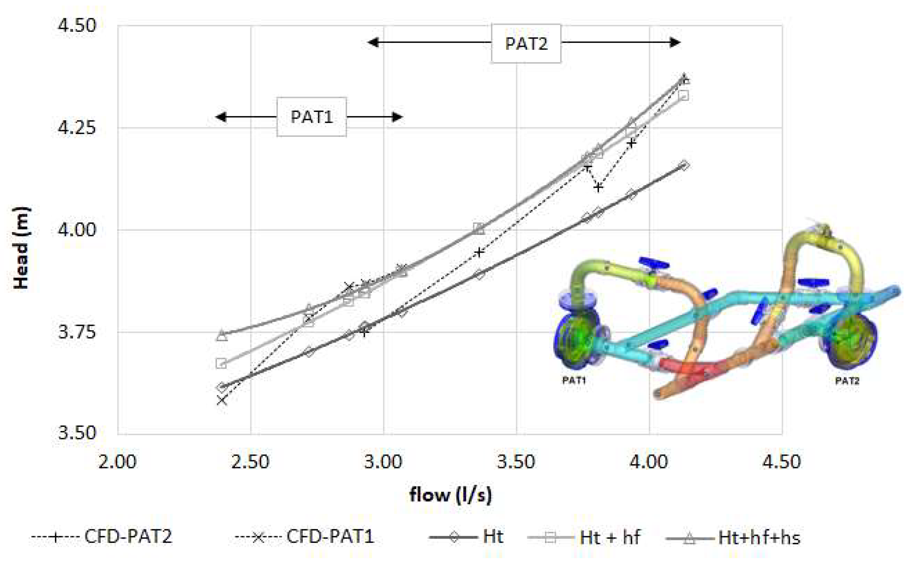
In order to understand the behavior of the flow inside the machine, the pressure loss was studied to estimate the head provided by each PAT when installed in parallel. Based on Figure 12, the recovered head can be discretized by Equation (8):
where is the head (m.wc.); is the theoretical recovered head considering the Euler equation (m.wc.).
Table 2 shows three formulations based on experiments to determine the theoretical head, the impeller friction losses, and the shock losses. These formulations were adopted according to the literature [27,33,34,35].
In order to check the validity of the CFD model, a comparison between these empirical formulations, as shown in Table 2, and the head losses obtained inside the two impellers based on CFD simulations were established, as shown in Figure 16. The impeller shock losses present a smaller impact on the head stage compared to the friction losses. The lowest losses were reached when the shock losses within the impeller were the smallest (points 4 and 12 from Figure 15). The results from the CFD model indicate that the overall performance of the two runners was in the range of performance variation by the empirical models presenting reduced errors (between 0.2‒2% for PAT 1 and 0.4‒4% for PAT2).
5.3. Comparisons
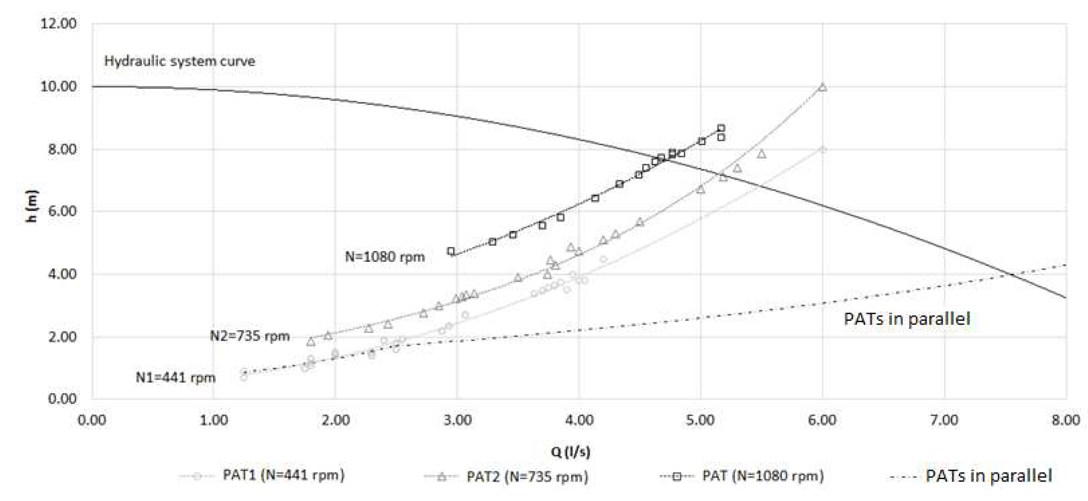
When the flow is different from the normal rated conditions, two PATs in parallel can better cover it. When setting up the system with two PATs in parallel it is possible to run the system for low and medium flow rates with PAT1 or PAT2 or using together for a large flow rate with both PATs in operation. From the EPANET model, the installation curve of the system was defined, as shown in Figure 17, and used to calculate the operating point of the two PATs running in parallel against one single PAT. For the H-Q curve of PATs in parallel, for 1.25 L/s < Q < 2.80 L/s is equal to the H-Q curve of PAT1, since the characteristic curve of PAT2 does not reach the head of PAT1. For Q > 2.5 L/s the H-Q curve for PATs in parallel is obtained by adding the flow rates and contributions from each PAT at the system head, resulting, in this case, an operating point of Q = 7.6 L/s and H = 4 m. The increasing of head losses in the PATs during parallel system is prominent, with the increasing of the flow conditions.
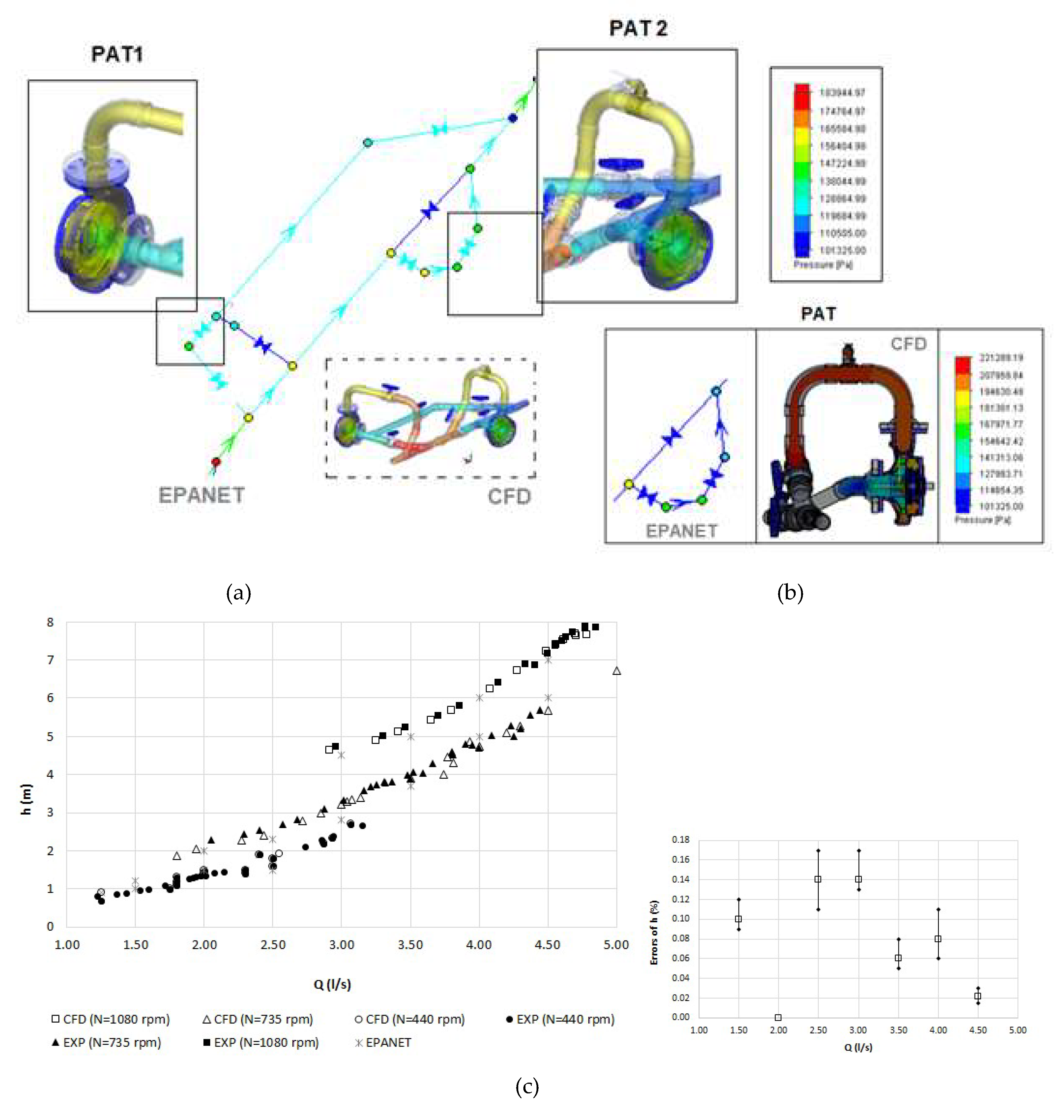
Comparing the head losses achieved in the EPANET (1D) and in the CFD (3D) models, the 1D results show good accordance with experiments in terms of pressure and flow rates. The average head losses given by EPANET from upstream to downstream of PAT1 and PAT2, as shown in Figure 18, running in parallel, are about 1.5 m, against 1.9 m from the CFD model and 1.8 m from experiments. Switching into single mode, where the flow rate is reduced, the head losses between the upstream and downstream of the runner correspond to the increasing of the net head. The slight mismatch between numerical modelling and experimental results was due to certain uncertainties in the CFD model (e.g., geometry, partial dissipation), which shows an error range between 3% and 17%.
Not only the geometry differences between real PATs and models, but also the typology of the system, contributes to the percentage of the head drop and the evaluation of local head losses during the simulations. Also, these mechanical losses were associated to the scale effect frictions and bearings, the surface roughness of the tested model, shock and leakages between the impeller and the case, and the eventually entrapped air associated with bubbles, responsible for additional turbulence and swirl effects.
Nevertheless, the PAT’s head provided by both models, such as in EPANET and 3D CFD models, was quite similar to the collected experiments, showing the ability of both models to analyze accurately, depending on the degree of detail required (i.e., along the pipe system—EPANET, inside the PAT system configuration—CFD).
6. Conclusions
This research improves the understanding of PAT systems where the flow varies along with time. From established PAT theory, the testing operation of two PATs used in parallel and in single mode were analyzed. As a new idea, the research developed experimental and numerical analyses using different PAT behavior in a single and in parallel modes with different rotational speeds. This analysis contributes to improve the behavior of PAT systems in order to search the best operating conditions associated with water distribution systems. The analysis studied the characteristic curves (i.e., H-Q and η–Q for different N) as well as the variation of the head losses in each PAT system.
Experimental tests were developed for different rotational speeds in each PAT according to input data conditions. Experimental measurements (i.e., flow rate, rotational speed, and pressure) were transferred to the simulation models. The calibration was conducted under steady state conditions, comparing the simulated and experimental losses in several monitor points distributed along the PATs’ control volume. The main conclusions can be summarized as follows:
- (1)
- The characteristic curves were rather different from PAT1 to PAT2 due to different rotational speeds and flow rates, associated to each PAT, even for equal machines working in parallel mode;
- (2)
- During the steady state operating condition, in the parallel configuration, the optimal point was obtained for a total flow of Q =7.50 L/s and H = 4 m; corresponding to Q = 4.00 L/s for PAT1 and Q = 3.53 L/s for PAT2, associated to N1 = 440 rpm and N2 = 735 rpm, respectively;
- (3)
- Although parallel operation increases the total flow rate, it also causes greater head losses, with a reduction in the flow rate in each PAT, and consequentially, alterations in the efficiency of each PAT;
- (4)
- In the CFD model, the head losses can be estimated in accordance with empirical formulations, with acceptable errors, allowing a better comprehension of the flow pattern inside the PAT system;
- (5)
- The benefits of PATs working in parallel are the possibility for covering higher flow range conditions than for a single PAT.
- (6)
- Comparing the CFD model with experimental tests, the optimal point for total flow during numerical simulations was achieved for Q = 7.6 L/s and H = 4 m. Also, the predicted flow rates were in good agreement with the measured data, presenting an average error of 10%.
This research contributes to improve the knowledge (experimental and numerical) in PAT systems when they are operating in parallel mode. This is a crucial point, since there is still a reduced amount of published research considering the experimental operation of PAT systems, and this is the first in parallel mode. The developed analyses show the need to calibrate the simulation models (such as CFD and EPANET) in order to develop suitable energy analyses in the water sector. These analyses will contribute as interesting tools for water managers to increase the efficiency of water supply systems, considering the total head losses, in the estimation of the available net head and associated energy production. The research has shown these losses are non-negligible, depending on the system configuration and when the flow is out of the best efficiency point.
Author Contributions
The author H.M.R. has contributed the idea. H.M.R. and A.C. have contributed the revision of the document, and the supervising of the research. M.P.-S. contributed to describe the results and conclusions. M.S. conceived the experimental tests, conceived and developed the numerical modelling, and the analysis of results.
Funding
This research was funded by project REDAWN (Reducing Energy Dependency in Atlantic Area Water Networks) EAPA_198/2016 from INTERREG ATLANTIC AREA PROGRAMME 2014-2020.
Acknowledgments
The authors wish to thank to the project REDAWN (Reducing Energy Dependency in Atlantic Area Water Networks) EAPA_198/2016 from INTERREG ATLANTIC AREA PROGRAMME 2014-2020, CERIS and the DECivil Hydraulic Laboratory, for the support in the developments and the experiments on pumps working as turbines.
Conflicts of Interest
The authors declare no conflict of interest.
References
- Ismail, M.A.; Othman, A.K.; Islam, S.; Zen, H. End suction centrifugal pump operating in turbine mode for microhydro applications. Adv. Mech. Eng. 2015, 7. [Google Scholar] [CrossRef]
- Jain, S.V.; Patel, R.N. Investigations on pump running in turbine mode: A review of the state-of-the-art. Renew. Sustain. Energy Rev. 2014, 30, 841–868. [Google Scholar] [CrossRef]
- Darmawi, R.; Sipahutar, S.M.; Bernas, M.S.; Imanuddin, M.S. Renewable energy and hydropower utilization tendency worldwide. Renew. Sustain. Energy Rev. 2013, 17, 213–215. [Google Scholar] [CrossRef] [Green Version]
- García, I.F.; Ferras, D.; Mc Nabola, A. Potential of energy recovery and water saving using micro-hydropower in rural water distribution networks. J. Water Resour. Plann. Manag. 2019, 145, 05019001. [Google Scholar] [CrossRef]
- Ramos, H.; Borga, A. Pumps as turbines: An unconventional solution to energy production. Urban Water 1999, 1, 261–263. [Google Scholar] [CrossRef]
- Williams, A.A. Pumps as turbines for low cost micro hydropower. Renew. Energy 1996, 9, 1227–1234. [Google Scholar] [CrossRef]
- Motwani, K.H.; Jain, S.V.; Patel, R.N. Cost analysis of pump as turbine for pico hydropower plants—A case study. Procedia Eng. 2013, 51, 721–726. [Google Scholar] [CrossRef]
- Orchard, B.; Klos, S. Pumps as turbines for water industry. World Pumps 2009, 2009, 22–23. [Google Scholar] [CrossRef]
- Yang, S.S.; Derakhshan, S.; Kong, F.Y. Theoretical, numerical and experimental prediction of pump as turbine performance. Renew. Energy 2012, 48, 507–513. [Google Scholar] [CrossRef]
- Pérez-Sánchez, M.; López-Jiménez, P.; Ramos, H.M. Modified affinity laws in hydraulic machines towards the best efficiency line. Water Resour. Manag. 2018, 3, 829–844. [Google Scholar] [CrossRef]
- Pérez-Sánchez, M.; Sánchez-Romero, F.J.; López-Jiménez, P.; Ramos, H.M. PATs selection towards sustainability in irrigation networks: Simulated annealing as a water management tool. Renew. Energy 2018, 116, 234–249. [Google Scholar] [CrossRef]
- Alatorre-Frenk, C. Cost Minimisation in Micro-Hydro Systems Using Pumps-as-Turbines; University of Warwick: Coventry, UK, 1994. [Google Scholar]
- Carravetta, A.; Derakhshan, S.; Ramos, H.M. Pumps as Turbines, Fundamentals and Applications; Springer International Publishing: New York, NY, USA, 2018; ISSN 2195-9862. [Google Scholar]
- Spangler, D. Centrifugal pumps in reverse. An alternative to conventional turbines. Water Wastewater Int. 1988, 3, 13–17. [Google Scholar]
- Ramos, H. Guidelines for Design of Small Hydropower Plants; Western Regional Energy Agency & Network: Belfast, UK, 2000; ISBN 972 96346 4 5. [Google Scholar]
- Pérez-Sánchez, M.; Simão, M.; López-Jiménez, P.; Ramos, H.M. CFD analyses and experiments in a PAT modeling: Pressure variation and system efficiency. Fluids 2017, 2, 51. [Google Scholar] [CrossRef]
- Chapallaz, G.; Eichenberger, J.M.; Fischer, P. Manual on Pumps Used as Turbines; Vieweg: Braunschweig, Germany, 1992. [Google Scholar]
- Ramos, H.M.; Almeida, A.B. Dynamic orifice model on waterhammer analysis of high and medium heads of small hydropower schemes. J. Hydraul. Res. 2001, 39, 429–436. [Google Scholar] [CrossRef]
- Derakhshan, S.; Nourbakhsh, A. Experimental study of characteristic curves of centrifugal pumps working as turbines in different specific speeds. Exp. Therm. Fluid Sci. 2008, 32, 800–807. [Google Scholar] [CrossRef]
- Simão, M.; Pérez-Sánchez, M.; Carravetta, A.; López-Jiménez, P.; Ramos, H.M. Velocities in a centrifugal PAT operation: Experiments and CFD analyses. Fluids 2017, 3, 3. [Google Scholar] [CrossRef]
- Vieira, T.S.; Siqueira, J.R.; Bueno, A.D.; Morales, R.; Estevam, V. Analytical study of pressure losses and fluid viscosity effects on pump performance during monophase flow inside an ESP stage. J. Pet. Sci. Eng. 2015, 127, 245–258. [Google Scholar] [CrossRef]
- Fecarotta, O.; Aricò, C.; Carravetta, A.; Martino, R.; Ramos, H.M. Hydropower potential in water distribution networks: Pressure control by PATs. Water Resour. Manag. 2015, 29, 699–714. [Google Scholar] [CrossRef]
- Carravetta, A.; Giudice, G.; Fecarotta, O.; Ramos, H.M. Pump as turbine (PAT) design in water distribution network by system effectiveness. Water 2013, 5, 1211–1225. [Google Scholar] [CrossRef]
- Agarwal, T. Review of pump as turbine (PAT) for micro-hydropower. Int. J. Emerg. Technol. Adv. Eng. 2012, 2, 163–169. [Google Scholar]
- Derakhshan, S.; Mohammadi, B.; Nourbakhsh, A. Efficiency improvement of centrifugal reverse pumps. J. Fluids Eng. 2009, 131, 211039. [Google Scholar] [CrossRef]
- Rossman, L.A. EPANET 2 User’s Manual; U.S. Environmental Protection Agency (EPA): Cincinnati, OH, USA, 2000.
- Fecarotta, O.; Carravetta, A.; Ramos, H.M.; Martino, R. An improved affinity model to enhance variable operating strategy for pumps used as turbines. J. Hydraul. Res. 2016, 54, 332–341. [Google Scholar] [CrossRef]
- Buono, D.; Frosina, E.; Mazzone, A.; Cesaro, U.; Senatore, A. Study of a pump as turbine for a hydraulic urban network using a tridimensional CFD modeling methodology. Energy Procedia 2015, 82, 201–208. [Google Scholar] [CrossRef]
- Mentor Graphics Corporation. FloEFD Technical Reference; Mentor Graphics Corporation: Wilsonville, OR, USA, 2011. [Google Scholar]
- Abilgaziyev, A.; Nogerbek, N.; Rojas-Solórzano, L. Design optimization of an oil-air catch can separation system. J. Transp. Technol. 2015, 5, 15. [Google Scholar] [CrossRef]
- Ramos, H.M.; Almeida, A.B. Dynamic effects in micro-hydro modelling. Int. Water Power Dam Constr. 2003, 55, 22–25. [Google Scholar]
- Frosina, E.; Dario, B.; Senatore, A. A Performance prediction method for Pumps as Turbines (PAT) using a Computational Fluid Dynamics (CFD) modeling approach. Energies 2017, 10, 103. [Google Scholar] [CrossRef]
- Sun, D.; Prado, M.G. Single-phase model for ESP’s performance. In Proceedings of the TUALP Annual Advisory Board Meeting, Tulsa/Oklahoma, Oklahoma City, OK, USA, 23‒26 March 2002; p. 42. [Google Scholar]
- Thin, K.C.; Khaing, M.; Aye, K.M. Design and performance analysis of centrifugal pump. World Acad. Sci. Eng. Technol. China 2008, 46, 422–429. [Google Scholar]
- Bing, H.; Tan, L.; Cao, S.L.; Lu, L. Prediction method of impeller performance and analysis of loss mechanism for mixed-flow pump. Sci. China Technol. Sci. 2012, 55, 1988–1998. [Google Scholar] [CrossRef]
Figure 1.
Identification of hydraulic losses in a pump as turbine (PAT).

Figure 2.
Experimental set-up at IST (DECivil-Lab).

Figure 3.
PATs’ characteristic operating points when working in parallel and in a single mode: (a) h curve; (b) N curve.
Figure 3.
PATs’ characteristic operating points when working in parallel and in a single mode: (a) h curve; (b) N curve.

Figure 4.
Identification of experimental characteristic curves: (a) PATs working in parallel mode (with 270 rpm ≤ PAT1 ≤ 441 rpm and 747 rpm ≤ PAT2 ≤ 800 rpm); (b) one PAT working in single mode (725 rpm ≤ PAT ≤ 1080 rpm).
Figure 4.
Identification of experimental characteristic curves: (a) PATs working in parallel mode (with 270 rpm ≤ PAT1 ≤ 441 rpm and 747 rpm ≤ PAT2 ≤ 800 rpm); (b) one PAT working in single mode (725 rpm ≤ PAT ≤ 1080 rpm).

Figure 5.
Parallel PATs in operation: (a) global system of two PATs in parallel: scenario 1—total flow range between 5.80 L/s and 6.60 L/s, and scenario 2—total flow range between 6.70 L/s and 7.20 L/s; (b) scenario 1 by each PAT; (c) scenario 2 by each PAT.
Figure 5.
Parallel PATs in operation: (a) global system of two PATs in parallel: scenario 1—total flow range between 5.80 L/s and 6.60 L/s, and scenario 2—total flow range between 6.70 L/s and 7.20 L/s; (b) scenario 1 by each PAT; (c) scenario 2 by each PAT.

Figure 6.
Experimental PATs’ operating conditions used in the CFD model.

Figure 7.
Schematic of the experimental set-up in EPANET. CV: check valve; FCV: flow control valves; GPV: general purpose valves.
Figure 7.
Schematic of the experimental set-up in EPANET. CV: check valve; FCV: flow control valves; GPV: general purpose valves.

Figure 8.
Calibration of the network: (a) scenario 1—Q = 5.81 L/s; (b) scenario 2—Q = 6.77 L/s.

Figure 9.
Computational fluid dynamics (CFD) model: (a) defined mesh; (b) convergence of maximum static pressure results vs. different number of mesh cells.
Figure 9.
Computational fluid dynamics (CFD) model: (a) defined mesh; (b) convergence of maximum static pressure results vs. different number of mesh cells.

Figure 10.
PAT system set-up: (a) fluid volume in PATs operating in parallel; (b) PAT geometry mesh.
Figure 10.
PAT system set-up: (a) fluid volume in PATs operating in parallel; (b) PAT geometry mesh.

Figure 11.
Performance of PATs working in parallel (PAT1 and PAT2) mode.

Figure 12.
Pressure variation of the single PAT2 operation for the best efficiency point (BEP) (a); and for the parallel mode (N1 = 440 rpm and Q1 = 2.93 L/s) for PAT1 and (N2 = 735 rpm and Q2 = 3.77 L/s) for PAT2 (b).
Figure 12.
Pressure variation of the single PAT2 operation for the best efficiency point (BEP) (a); and for the parallel mode (N1 = 440 rpm and Q1 = 2.93 L/s) for PAT1 and (N2 = 735 rpm and Q2 = 3.77 L/s) for PAT2 (b).

Figure 13.
Velocity streamlines for: (a) Q = 5.80 L/s with N1 = 400 rpm and N2 = 700 rpm; (b) Q = 6.70 L/s with N1 = 440 rpm and N2 = 735 rpm; (c) Q = 7.20 L/s with N1 = 440 rpm and N2 = 735 rpm (with PAT1 on the left, PAT2 on the right).
Figure 13.
Velocity streamlines for: (a) Q = 5.80 L/s with N1 = 400 rpm and N2 = 700 rpm; (b) Q = 6.70 L/s with N1 = 440 rpm and N2 = 735 rpm; (c) Q = 7.20 L/s with N1 = 440 rpm and N2 = 735 rpm (with PAT1 on the left, PAT2 on the right).

Figure 14.
Location of monitor points in the control volume between inlet and outlet of PATs.

Figure 15.
Head losses at monitor points along the PATs system for different total flow values.

Figure 16.
Hydraulic losses distribution in each PAT.

Figure 17.
Operation of PATs working in parallel (PAT1, PAT2, and PATs) and in single mode (PAT).

Figure 18.
Head losses determined in parallel mode (a) and in single mode (b). Comparison between experimental results and modeling predictions with the associated errors (c).
Figure 18.
Head losses determined in parallel mode (a) and in single mode (b). Comparison between experimental results and modeling predictions with the associated errors (c).


Table 1.
Experimental tests. Q: discharge; N: rotational speed; h: net head.
| Condition | QPAT1 (L/s) | QPAT2 (L/s) | NPAT1 (rpm) | NPAT2 (rpm) | h PAT1 (m) | h PAT2 (m) |
|---|---|---|---|---|---|---|
| PATs in Parallel | 2.66 | 3.94 | 284 | 816 | 1.80 | 5.05 |
| 2.93 | 3.93 | 427 | 812 | 2.34 | 4.88 | |
| 2.56 | 3.74 | 300 | 725 | 1.66 | 4.00 | |
| 2.39 | 4.81 | 250 | 1083 | 1.34 | 7.93 | |
| 2.93 | 4.07 | 427 | 813 | 2.34 | 5.04 | |
| 2.39 | 3.81 | 250 | 754 | 1.34 | 4.30 | |
| 3.07 | 3.93 | 497 | 772 | 2.70 | 4.87 | |
| 2.93 | 3.77 | 427 | 735 | 2.34 | 4.45 | |
| 3.07 | 4.13 | 497 | 875 | 2.70 | 5.59 | |
| 2.87 | 2.93 | 400 | 427 | 2.19 | 2.34 | |
| 3.40 | 4.20 | 520 | 860 | 2.04 | 4.80 | |
| 3.00 | 4.10 | 300 | 880 | 1.31 | 4.01 | |
| 2.80 | 3.46 | 280 | 680 | 1.26 | 2.90 | |
| 3.40 | 4.50 | 570 | 950 | 1.98 | 4.82 | |
| 2.50 | 4.20 | 230 | 880 | 1.37 | 4.70 | |
| 2.75 | 4.00 | 300 | 850 | 1.47 | 4.30 | |
| 2.10 | 4.03 | 190 | 935 | 1.33 | 4.23 | |
| 2.50 | 3.42 | 205 | 600 | 1.29 | 4.10 | |
| 2.95 | 3.35 | 350 | 600 | 2.26 | 3.85 | |
| 2.05 | 1.14 | 440 | 735 | 1.40 | ||
| 2.16 | 1.31 | 1.50 | ||||
| 2.45 | 1.73 | 1.80 | ||||
| 2.63 | 1.96 | 2.00 | ||||
| 2.95 | 2.36 | 2.40 | ||||
| 3.24 | 2.71 | 2.80 | ||||
| 3.38 | 2.87 | 3.00 | ||||
| 3.52 | 3.02 | 3.20 | ||||
| 3.64 | 3.16 | 3.40 | ||||
| 3.77 | 3.30 | 3.60 | ||||
| 3.89 | 3.43 | 3.80 | ||||
| 4.00 | 3.56 | 4.00 | ||||
| 4.12 | 3.69 | 4.20 | ||||
| 4.23 | 3.81 | 4.40 | ||||
| 2.39 | 3.26 | 270 | 830 | 1.34 | 3.90 | |
| 2.66 | 3.11 | 1.80 | 3.63 | |||
| 2.56 | 2.78 | 1.66 | 3.14 | |||
| 2.00 | 2.60 | 1.00 | 2.97 | |||
| 1.80 | 2.22 | 0.90 | 2.69 | |||
| 2.00 | 2.90 | 1.05 | 3.29 | |||
| 2.20 | 2.48 | 1.50 | 2.85 | |||
| 2.75 | 3.42 | 1.50 | 4.19 | |||
| Single PAT | 3.81 | 725 | 4.54 | |||
| 3.95 | 724 | 4.78 | ||||
| 4.09 | 725 | 5.03 | ||||
| 4.23 | 726 | 5.29 | ||||
| 4.80 | 980 | 7.22 | ||||
| 4.42 | 980 | 6.82 | ||||
| 4.80 | 979 | 7.46 | ||||
| 4.17 | 980 | 6.20 | ||||
| 4.34 | 1080 | 8.26 | ||||
| 4.80 | 1080 | 8.38 | ||||
| 4.76 | 1081 | 7.91 | ||||
| 4.95 | 1150 | 8.66 | ||||
| 4.49 | 1079 | 7.19 | ||||
Table 2.
Formulations to estimate the head of PAT [26].
Table 2.
Formulations to estimate the head of PAT [26].
| Ref. | Parameter | Formula | Complement |
|---|---|---|---|
| [31,32,33,34] | net theoretical head (Ht) | ||
| [31,33] | friction loss (hf) | ||
| [34] | shock loss (hs) | kshock = 0.2 |
Subscripts 1 and 2 represent the inlet and outlet of the impeller; β—blade angle; Na—number of channels between blades; b—channel width.
© 2019 by the authors. Licensee MDPI, Basel, Switzerland. This article is an open access article distributed under the terms and conditions of the Creative Commons Attribution (CC BY) license (http://creativecommons.org/licenses/by/4.0/).
Share and Cite
MDPI and ACS Style
Simão, M.; Pérez-Sánchez, M.; Carravetta, A.; Ramos, H.M. Flow Conditions for PATs Operating in Parallel: Experimental and Numerical Analyses. Energies 2019, 12, 901. https://doi.org/10.3390/en12050901
AMA Style
Simão M, Pérez-Sánchez M, Carravetta A, Ramos HM. Flow Conditions for PATs Operating in Parallel: Experimental and Numerical Analyses. Energies. 2019; 12(5):901. https://doi.org/10.3390/en12050901
Chicago/Turabian StyleSimão, Mariana, Modesto Pérez-Sánchez, Armando Carravetta, and Helena M. Ramos. 2019. "Flow Conditions for PATs Operating in Parallel: Experimental and Numerical Analyses" Energies 12, no. 5: 901. https://doi.org/10.3390/en12050901
Note that from the first issue of 2016, this journal uses article numbers instead of page numbers. See further details here.