A Model to Predict Crosscut Stress Based on an Improved Extreme Learning Machine Algorithm


1
Intelligent Mine Research Center, Northeastern University, Shenyang 110004, China
2
School of Civil Engineering, The University of Sydney, Sydney, NSW 2006, Australia
*
Author to whom correspondence should be addressed.
Energies 2019, 12(5), 896; https://doi.org/10.3390/en12050896
Submission received: 8 February 2019
/
Revised: 28 February 2019
/
Accepted: 28 February 2019
/
Published: 7 March 2019
Abstract
:The analysis of crosscut stability is an indispensable task in underground mining activities. Crosscut instabilities usually cause geological disasters and delay of the project. On site, mining engineers analyze and predict the crosscut condition by monitoring its convergence and stress; however, stress monitoring is time-consuming and expensive. In this study, we propose an improved extreme learning machine (ELM) algorithm to predict crosscut’s stress based on convergence data, for the first time in literature. The performance of the proposed technique is validated using a crosscut response by means of the FLAC3D finite difference program. It is found that the improved ELM algorithm performs higher generalization performance compared to traditional ELM, as it eliminates the random selection for input weights. Furthermore, a crosscut construction project in an underground mine, Yanqianshan iron mine, located in Liaoning Province (China), is selected as the case study. The accuracy and efficiency of the improved ELM algorithm has been demonstrated by comparing predicted stress data to measured data on site. Additionally, a comparison is conducted between the improved ELM algorithm and other commonly used artificial neural network algorithms.
Keywords:
crosscut; stress; convergence; artificial neural network; extreme learning machine; FLAC3D1. Introduction
Surrounding rock stability in crosscuts has always been a major concern in underground mining activities. Crosscut accidents such as roof failures, rib falls, and rock blasts primarily resulted from stress concentration and could lead to casualties and huge economic loss [1,2,3,4]. For example, major roof failures in Australian underground mines have been known to result in the stoppage of crosscut construction for several months, causing a production loss of more than a hundred million dollars in some cases [5]. Generally, the crosscut stability can be monitored and predicted by analyzing stress and displacement in surrounding rock. In situ, the displacement of surrounding rock can be measured efficiently and economically by convergence instruments, such as tape extensometers, laser scanners (profilometers), and geodetic surveying (total stations) [6]. These instruments are usually placed at intervals between 5 m and 50 m relying on the rock properties. The convergence data of surrounding rock is processed manually or automatically as digital data and then transmitted to the data processing unit [7,8]. However, it is time-consuming and expensive to obtain the stress data of surrounding rock in crosscuts. Additionally, the stress-deformation relationship for surrounding rock in crosscuts is full of uncertainty, as it is affected by many factors such as lithology, rock mass structure, and groundwater [9,10]. Hence, it is of great practical significance to seek a commercially available way to obtain the stress distribution of surrounding rock in crosscuts.
Recently, artificial neural networks (ANN) have been applied extensively in tunnel displacement prediction [6], as it is an efficient identification method for its non-linear transformation and highly parallel computing. ANN has the advantages of reducing interference from irrelevant factors, using a specific set of criteria, considering lots of quantitative and qualitative factors and ensuring accuracy compared to traditional methods [11,12]. Flood and Kartam [13] introduced the application of ANN in civil engineering. Kim et al. [14] predicted the ground settlement resulting from tunnel excavation by using the neural network. Zhou and Li [15] used nonlinear support vector machines (SVM) and multiple linear regression models to evaluate the thickness of broken rock zone for deep crosscuts. Pourtaghi et al. [16] integrated the wavelet theory and ANN to predict maximum surface settlement caused by tunneling. Lai et al. [17] incorporated the ANN into predicting the soil deformation in tunnels. Chen et al. [18] used ANN optimized by the genetic algorithm to predict the collapse depth of thin-layered rock strata during tunneling, and the absolute error between predicted and measured collapse depths was less than 15%. Reported literatures have highlighted the application of ANN in predicting the displacement of surrounding rock in crosscuts. However, using ANN to predict stress based on displacement data is scare.
Gradient-based learning methods such as backpropagation (BP) neural network are usually adopted in ANN schemes, but problems (i.e., over-tuning, local minima, stopping criteria, and long computation time) existed [19]. To overcome these difficulties, a relatively novel algorithm for single-hidden-layer feedforward neural network called the Extreme Learning Machine (ELM) has been proposed recently in References [20,21]. The input weights and hidden biases in traditional ELM are randomly chosen, and the output weights are analytically determined by using Moore-Penrose generalized inverse. The input weights link the input layer to the hidden layer, while the output weights link the hidden layer to the output layer. ELM is a powerful classification model with extremely fast learning capacity and good generalization performance compared to traditional gradient-based learning method. Thus, ELM has been widely applied in many fields with its variants. For example, Yeu et al. [22] evaluated the performance of ELM on multiresolution access of terrain height information. Lian et al. [23] used the modified ensemble empirical mode decomposition-based ELM model to predict landslide displacement. They noticed the prediction obtained from ELM was consistently better than basic ANN. Li et al. [24] investigated the rock slope stability by using the extreme learning neural network and terminal steepest descent algorithm. Zhang et al. [25] evaluated the ELM performance on multicategory classification. Their results indicated that ELM produced comparable or better accuracies with reduced training time and implementation complexity compared to ANN and support vector machine methods.
However, the randomly assigned input weights and biases usually bring certain randomness and then reduce the generalization ability of ELM [26]. Several studies have worked on improve the generalization performance of traditional ELM. Liao and Feng [27] proposed a meta-ELM method to train the training data with base ELM hidden nodes, instead of using the ensemble method. They found the Meta-ELM is more feasible and effective compared to traditional ELM. Yadav et al. [28] used particle swarm combined with ELM to estimate the in-situ bioremediation system cost. Deng et al. [29] used a Fast SVD-Hidden-nodes based Extreme Learning Machine for determining the input weights and large-scale data analytics.
To the best of our knowledge, the application of ELM for stress prediction in crosscut’s surrounding rock is limited in the literature. In this paper, we develop an improved ELM by employing greedy algorithm, which could improve the unsatisfactory generalization performance of traditional ELM resulting from random selection for input weights. The improved ELM could be used as an effective and accurate prediction method to provide accurate information about stress data for surrounding rock and to analyze crosscut stability. A brief introduction on the traditional ELM is presented in Section 2. Section 3 introduces the algorithm of improved ELM, followed by a validation of its improvement using a crosscut response (Section 4) and its engineering application (Section 5). A comparison between improved ELM and other existing ANN algorithms is also conducted in Section 5. Finally, the conclusion drawn from the present study is summarized in Section 6.
2. A Brief Introduction to Traditional ELM
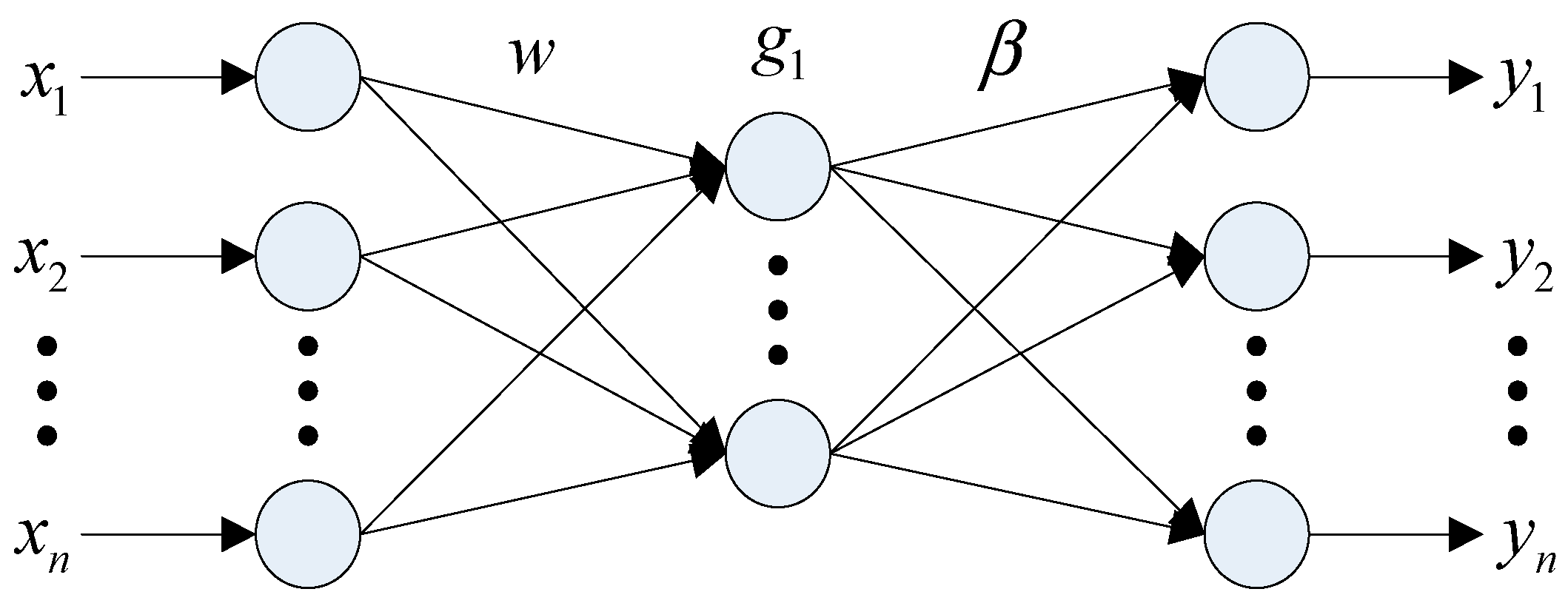
ELM is a typical single-hidden-layer feedforward neural network (SLFN). Unlike traditional learning algorithms in feedforward neural network where the parameters are tuned iteratively, ELM calculates the hidden layer node parameters mathematically, resulting in good generalization ability at extremely fast learning speed [30]. Structure of ELM is illustrated in Figure 1.
For N arbitrary distinct samples , where and , standard SFLN with hidden neurons and activation function g(x) are mathematically modelled as [30]:
where is the weight of the connection from the input neurons to the ith hidden neuron; is the weight vector connecting the ith output neurons and hidden neuron; is the jth output vector of SLFN; is the threshold of the ith hidden neuron; and presents the inner product of and .
Equation (1) can be written compactly as:
where
where H is the hidden–layer output matrix of the neural network. The ith column of H is the ith hidden nodes output vector corresponding to inputs x1, …, xN, and the jth row of H is the output vector of the hidden layer with respect to inputs xj.
The input weight wi and hidden biases bi is chosen randomly without knowing the training datasets. The output weight L is then solved with matrix computation formula = H+T, where H+ is Moore-Penrose of H and is the target value matrix. ELM not only tends to find the smallest norm weights, but also the smallest training error, and its pseudo code is shown in Algorithm 1 [20].
| Algorithm 1. Algorithm for traditional extreme learning machine |
| 1: for i = 1 to do |
| 2: randomly assign input weight wi |
| 3: randomly assign hidden bias bi |
| 4: calculate H |
| 5: calculate β = H+T |
3. Improved ELM Algorithm
As discussed earlier, the input weight of traditional ELM is random usually causing low generalization ability. Therefore, the greedy algorithm is firstly employed into this study to improve the generalization performance of traditional ELM. When solving the problem greedy algorithm always makes the best choice at present step and will consider local optimal solution rather than the overall optimization. The procedure of greedy algorithm includes four steps, e.g., (a) establishing a mathematical model to describe the problem, (b) dividing the problem into several sub-problems, (c) determining local optimal solution for each sub-problem, and (d) combining the all local optimal solutions [31]. The iteration process for greedy algorithm is summarized as follows. In the given dataset D and objective function f, the initial approximating value f0 is set at 0. The approximating value at kth iteration fk is determine based on fk−1, and the approximating error at (k − 1)th iteration τk−1 is calculated as f − fk. For each iteration, one is expected to reduce τk as much as possible. The analytical formula is expressed as
here
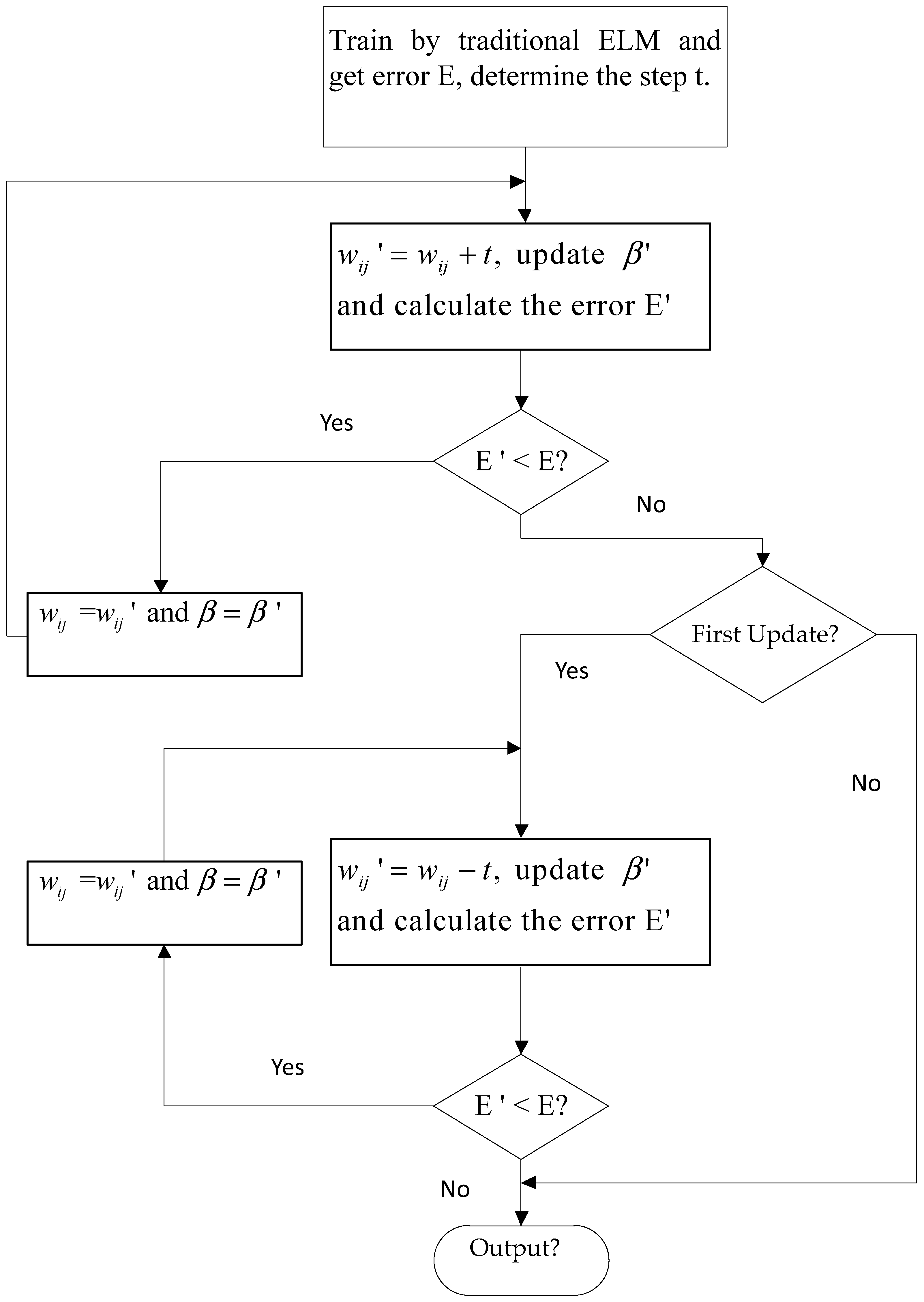
The incorporated greedy algorithm makes the traditional ELM system move in the direction of reducing the error when the error obtained from system cannot meet the requirement. Once the local minimum point is found, the searching step will be ended and then work on the rest data. Thus, the whole hidden layer can be changed with reducing the error significantly. Based on the traditional ELM model, the computational process for the improved ELM algorithm is shown in Figure 2.
The steps of constructing the crosscut stress prediction model are described as follows:
- (1)
- Establish relational model of stress-displacement based on traditional ELM.
- (2)
- Calculate the error E and determine the searching step t.
- (3)
- Modify input weight in hidden layer with t and get new input weight .
- (4)
- Update the new output layer weight β’.
- (5)
- Calculated the new error E’ and compare with old error E.
- (6)
- If E’ < E, and β’ replace previous parameters and then iterates.
- (7)
- If E’ > E in first change, the previous weight should be kept and then reverse lookup.
To illustrate the effectiveness of the proposed improved ELM algorithm, two studies including the numerical study and case study are presented in the following sections.
4. Verification with a Crosscut Response
4.1. Numerical Model
FLAC3D, which is a numerical software based on finite-difference method, has been widely used in mining engineering to analyze the ground subsidence and deformation and stress distribution of surrounding rock [32,33]. Based on FLAC3D, a three-dimensional model according to the mining condition was established to obtain stress-displacement data for ELM use, as shown in Figure 3, since the change of displacement in crosscuts is inconspicuous and difficult to get a lot of data in a short time [28].
As shown in Figure 3a, the model dimensions were taken as 20 m (−10 m~+10 m) on the X-axis, 35 m (0 m~35 m) on the Y-axis, and 20 m (−10 m~+10 m) on the Z-axis. The model has 32,436 nodes and 30,800 elements. In Figure 3b, the yellow part in the model middle is the tunnel which will be excavated. The width of tunnel is 4 m with a height of 3.8 m in a central line, and the radius in upper semi-circle part is 2.0 m. Six sampling points located in cross section between y = 5 m and y = 6 m to obtain stress-displacement data are illustrated in Figure 3c.
Another important part of numerical modelling is assigning the constitutive model, which describes the mechanical behaviour including yielding and post-crack of geomaterial [34]. In FLAC3D, elastic, strain softening, and Mohr-coulomb (mohr) models are often used for mining engineering. In this simulation, the mohr model is used to simulate the behaviour of surrounding rock (e.g., magnetite), since it can describe the granular materials with loose cementation in an ideal situation. Mechanical properties of magnetite simulated in this study are given in Table 1, based on laboratory tests and field investigations.
4.2. Data Collection
After crosscut excavation, the stress state balance in surrounding rock is disturbed. The displacement and stress will change with time until it reaches equilibrium. During the computational process, FLAC3D could record the displacement and stress information of monitoring points automatically. The displacement distribution in crosscut surrounding rock after excavation is shown in Figure 4. It can be noticed that the biggest settlement existed in the middle roof, which is corresponding to the monitoring point ID 21461 and ID 6061. Considering the difference of stress-displacement state between ID 21461 and ID 6061 is unremarkable, ID 21461 is chosen for ELM training and validation. The vertical stress and X, Y, and Z-direction displacements of ID 21461 are given in Figure 5. As shown, the displacement of ID 21461 in Y-direction is not significant compared to that in X and Z-directions. Additionally, the stability of a crosscut is usually influenced by the overlaying rock gravity and horizontal displacement in side-walls. Thus, the displacements in X and Z-directions of ID 21461 are taken as input, while the vertical stress of ID 21461 is considered as output.
To improve the accuracy of the ELM model, the displacement and stress data of the elements in the same position as ID 21461 along the Y axis in different cross sections, e.g., 10 < y < 11, 15 < y < 16, 20 < y < 25, 30 < y < 31 are chosen as training samples. The total number of training samples is 3000.
4.3. Traditional and Improved ELM Validation
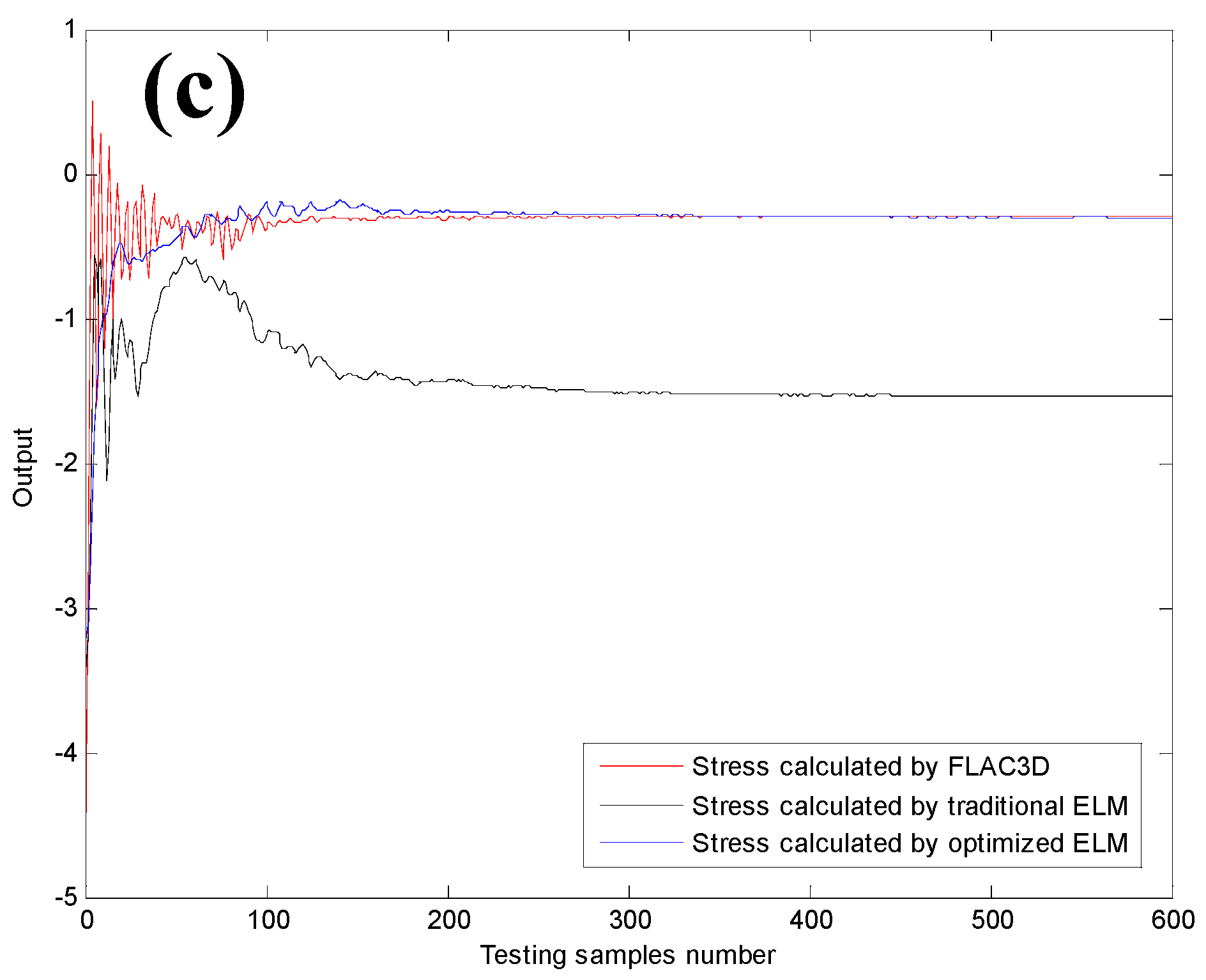
After training, the model is used to validate the vertical stress of elements in cross-sections 7 < y < 8, 13 < y < 14 and 17 < y < 18 according to their displacement data. By putting the displacement data obtained from X and Z-directions into the prediction model including traditional and improved ELM models, the relevant predictive vertical stress of elements can be obtained. Figure 6 compares the vertical stress obtained from two predictive models with measured data obtained from FLAC3D in three different cross-sections. It is worth noting that the vertical stress obtained from improved ELM model matches well with the results calculated by FLAC3D, regardless of the position of cross-section, especially for the residual stress. However, there is significant difference between traditional ELM predictions and numerical results.
To further validate the effectiveness and validity of the improved ELM model, additional vertical stress of 0.38 MPa was applied on the top surface of the numerical model to simulate increasing 10 m depth of the crosscut. Increasing depth leads to higher displacement and vertical stress in crosscut surrounding rock. During excavation of the crosscut, displacement information of elements in the middle roof in cross-sections 5 < y < 6, 10 < y < 11, 15 < y < 16, 20 < y < 21 was recorded and then employed into the improved ELM model. Figure 7 compares the vertical stress predicted by improved ELM model with that obtained from FLAC3D in four different cross-sections. As seen, the improved ELM model still predicts the vertical stress in high accuracy after changing the depth of excavated crosscut. Therefore, it may be concluded that the improved ELM algorithm is a promising technique to predict stress of surrounding rock in crosscut based on the displacement data. The improved ELM model will be applied in a case study of an underground crosscut in Yanqianshan Iron Mine.
5. Application to Yanqianshan Iron Mine
To illustrate its capability in engineering application, the improved ELM algorithm was used to predict the crosscut stress in Yanqianshan underground mine. The predictions from the improved ELM model were compared with the measured field data to evaluate the robustness of the proposed technique. In addition, the prediction performance of BP, ELM, genetic algorithm-based ELM (GA-ELM), and improved ELM were compared and discussed.
5.1. Engineering Background of Yanqianshan Iron Mine
Yanqianshan iron mine (YIM), located 22 km west of Anshan City, Liaoning Province, China, was commissioned in the 1960s. YIM includes three main orebodies (e.g., Fe1, Fe2, and Fe3) distributed in exploration lines from XVI to IX+100 as shown Figure 8. Fe1 is the main orebody with a strike length of 1600 m in the trans-meridional direction. Extraction procedure of YIM includes three parts, such as surface mining, transition stage mining, and underground mining. As shown in Figure 9, open-pit mining method with an annual production of 2.5 million ton was used in YIM between 1968 and 2012. The longest horizontal and vertical dimensions of pit are 1410 m and 710 m, respectively. The final pit depth is 276 m ranging from elevation −183 m to 93 m. Bench height is 12 m. For the transition stage, the target orebodies are ores in East and West hanging walls. The elevation of orebody in East-hanging wall ranges from −47 m and −123 m between exploration line VII-50~IX+100. The mining area in West-hanging wall starts from the exploration line XIV and ends at the west outskirts of open-pit with an orebody strike length ranging from 300 m to 550 m. For the underground mining stage, the mining depth is between −183 m and −500 m. The average thickness of underground orebody is 120 m with an average dip of 79°.
Currently, YIM is in the transition stage and mining the orebody in West hanging wall, which is also the case study in this paper. Drift-ramp and block caving method are selected to develop and extract the orebody in the West hanging wall. Two main haulages are constructed in level −51 m and −123 m, and the structural openings are in open-pit platform. The orebody is divided into 8 levels and each sublevel with a height of 18 m. Level +21 m is used to form the ore overburden layer. Considering the low stability of the hanging wall, there is a 20 m pillar between each ore layer and open-pit boundary.
5.2. Filed Data Collection
According to the geological condition and construction progress of West hanging wall, three monitoring areas were placed at #4, #5 and #6 crosscuts respectively on −33 m level, as shown in Figure 10a. Figure 10 also illustrates the drilling process for installing monitoring equipment. YHY200 borehole stress meter was used to record the stress variation. JSS30A Digital Display Convergence Meter with high precision was chosen to monitor the roof displacement, and tunnel section convergence continuous the monitoring system (TSCCMS) with a precision of 0.01 mm was used to record the horizonal displacement of surrounding rock. JSS30A and TSCCMS were placed near the location of borehole stress meter. The observation elapsed from January 2018 to March 2018, and data recorded every five days. A total number of 108 observations including 36 horizontal displacement values, 36 roof subsidence values, and 33 stress values were recorded, as shown in Figure 11.
As shown in the Figure 11a, it is clear that the convergence of these three crosscuts was between 4.9 mm and 8.2 mm. While there is slightly difference in convergence rate, the overall deformation law is similar, that is the crosscuts trend to convergent. The convergence rate is significantly dependent on mining progress. After drift blasting and excavation, the convergence value increases obviously. It is worth noting from Figure 11b, the roofs of these three monitored crosscuts performed deformation in different degrees, and the deformation value ranges from 0.77 mm to 2.47 mm. The monitoring points in #4 and #5 are influenced by mining activities, resulting in higher deformation in roof compared to that in #6. During the monitoring period, there were no extracting activities in #6. As shown in Figure 11c, the stress in monitored crosscuts has not changed distinctly with observed values between 0.18 MPa and 1.20 MPa. In general, the surrounding rock in the −33 m level could be kept stable during mining activities.
5.3. Training and Validation
The total number of collected vertical stress on the roof of crosscuts is 36 expressed as Z36. Accordingly, the measured convergence and roof displacements as shown in Figure 11a,b are named as X36 and Y36, respectively. The data is divided into training group (X24, Y24, and Z24) and validation group (X12, Y12, and Z12). After finishing training, X12 is incorporated into prediction models to obtain predictive results. For example, when validating the roof stress in #4 crosscut, the deformation including convergence and roof subsidence and roof stress of #5 and #6 crosscuts are selected as training data, while deformation of #4 crosscut is used as input. For comparison, the commonly used BP algorithms and GA-ELM are also used to predict crosscut stress.
To evaluate the prediction performance, three loss functions, namely root mean square error (RMSE), maximum relative error (MRE), and mean absolute percentage error (MAPE) are introduced as the evaluation criteria, as defined by Reference [23]
where ρ is the number of predictions; , is the in-situ data for time t, and is the predictive values for the same period.
The predicted stress of BP, ELM, GA-ELM, and improved ELM algorithms with the measured data in situ are compared in Figure 12 and Table 2. The training time, RMSE, MRE and MAPE of each algorithm are listed in Table 2 as well. As shown in Figure 12, we can find that predictions from the improved ELM model agree well with the field data in all crosscuts. GA-ELM model generally performs acceptable predictions on only #5 crosscut, but the prediction on the first 10 days still overestimate the field data significantly. The predictions of both BP and traditional ELM show are not accurate in all three cases. In general, four algorithms can predict the stress in crosscuts precisely at the beginning of monitoring. However, with times going by the predictions of BP, ELM, and GA-ELM gradually deviate the measured data in situ.
The results obtained from Table 2 obviously indicate that the prediction performance of the improved ELM model, is better than BP, ELM, and GA-ELM. The prediction precision of improved ELM has a significant improvement to traditional ELM where the RMSE, MRE, and MAPE reduce by 0.12MPa, 32.23%, and 15.94%, respectively. As expected the ELM shows the highest speed in prediction with a training time of 0.05 s, however, its performance is only slightly superior compared with BP. As for GA-ELM, although it performs acceptable precision with low RMSE (e.g., 0.13MPa), it is time-consuming compared with other three algorithms. In addition, the MRE obtained from GA-ELM is three times higher than that obtained from the improved ELM. The improved ELM algorithm computes quickly with a training time of only 1.70 s. Therefore, it can be concluded that the improved ELM algorithm is superior in predicting crosscut stress compared to BP, ELM, and GA-ELM.
6. Conclusions
Crosscut stability analysis has gained worldwide interests due to its importance in underground engineering projects. Stability analysis and prediction are commonly based on the crosscut convergence and stress data. However, it is time-consuming and expensive to monitor the crosscut stress. Therefore, an improved ELM algorithm is proposed in this paper to predict the crosscut stress using its convergence displacement. The capability of the improved ELM algorithm is then verified using a numerical model and a case study. The results show that traditional algorithm assigns input weight randomly leading to a fast computation speed, but unsatisfactory precision in stress prediction. The prediction accuracy and quality of ELM model was improved significantly by introducing greedy algorithm. In terms of different criteria, RMSE, MRE, and MAPE, it is found that for the test case of Yanqianshan Iron Mine, the improved ELM performs the best compared with BP, ELM, and GA-ELM algorithms. GA-ELM also shows acceptable prediction for #5 crosscut, however, it is time-consuming with a training time of 15.38 s, which is 14.37 times higher than that of the improved ELM algorithm. In conclusion, the improved ELM model can effectively improve the crosscut stress prediction and provide stability analysis for engineering projects, which is of great practical significance for future underground mining activities in Yanqianshan Iron Mine.
Author Contributions
X.L. proposed the improved algorithm; L.Y. set up the numerical experiments; X.Z. and L.W. collected the field data; X.L. and L.Y. finished the manuscript.
Funding
This work is financially funded by the Research Fund of National Natural Science Foundation of China (Grant No. 51674063) and the Fundamental Research Funds for the Central Universities (N170104017). The financial support is highly appreciated.
Conflicts of Interest
The authors declare that there is no conflict of interests regarding the publication of this paper.
References
- Qiu, J.P.; Yang, L.; Sun, X.G.; Xing, J. Strength characteristics and failure mechanism of cemented super-fine unclassified tailings backfill. Minerals 2017, 7, 58. [Google Scholar] [CrossRef]
- Yang, L.; Qiu, J.Q.; Jiang, H.Q.; Hu, S.Q.; Li, H.; Li, S. Use of cemented super-fine unclassified tailings backfill for control of subsidence. Minerals 2017, 7, 216. [Google Scholar] [CrossRef]
- Qiu, J.P.; Yang, L.; Xing, J.; Sun, X.G. Analytical Solution for Determining the Required Strength of Mine Backfill Based on its Damage Constitutive Model. Soil Mech. Found. Eng. 2018, 54, 371–376. [Google Scholar] [CrossRef]
- Yang, L.; Yilmaz, E.; Li, J.; Liu, H.; Jiang, H. Effect of superplasticizer type and dosage on fluidity and strength behavior of cemented tailings backfill with different solid contents. Constr. Build. Mater. 2018, 187, 290–298. [Google Scholar] [CrossRef]
- Shen, B.; King, A.; Guo, H. Displacement, stress and seismicity in crosscuts roofs during mining-induced failure. Int. J. Rock Mech. Min. Sci. 2008, 45, 672–688. [Google Scholar] [CrossRef]
- Adoko, A.C.; Jiao, Y.Y.; Wu, L.; Wang, H.; Wang, Z.H. Predicting tunnel convergence using multivariate adaptive regression spline and artificial neural network. Tunn. Undergr. Space Technol. 2013, 38, 368–376. [Google Scholar] [CrossRef]
- Kavvadas, M.J. Monitoring ground deformation in tunnelling: Current practice in transportation tunnels. Eng. Geol. 2005, 79, 93–113. [Google Scholar] [CrossRef]
- Simeoni, L.; Zanei, L. A method for estimating the accuracy of tunnel convergence measurements using tape distometers. Int. J. Rock Mech. Min. Sci. 2009, 46, 796–802. [Google Scholar] [CrossRef]
- Rogers, J.D.; Chung, J. Applying Terzaghi’s method of slope characterization to the recognition of Holocene land slippage. Geomorphology 2016, 265, 24–44. [Google Scholar] [CrossRef]
- Qiu, D.H.; Li, S.C.; Zhang, L.W.; Xue, Y.G. Application of GA-SVM in classification of surrounding rock based on model reliability examination. Min. Sci. Technol. 2010, 20, 428–433. [Google Scholar] [CrossRef]
- Abbas, M.; Morteza, B. Evolving neural network using a genetic algorithm for predicting the deformation modulus of rock masses. Int. J. Rock Mech. Min. Sci. 2010, 47, 246–253. [Google Scholar]
- Suchatvee, S.; Herbert, H.E. Artificial neural networks for predicting the maximum surface settlement caused by EPB shield tunneling. Tunn. Undergr. Space Technol. 2006, 21, 133–150. [Google Scholar]
- Flood, I.; Kartam, N. Neural networks in civil engineering I: Principles and understanding. J. Comput. Civ. Eng. 1994, 8, 131–148. [Google Scholar] [CrossRef]
- Kim, C.Y.; Bae, G.J.; Hong, S.W. Neural network based prediction of ground surface settlements due to tunneling. Comput. Geotech. 2001, 28, 517–547. [Google Scholar] [CrossRef]
- Zhou, J.; Li, X.B. Evaluating the Thickness of Broken Rock Zone for Deep Crosscuts using Nonlinear SVMs and Multiple Linear Regression Model. Procedia Eng. 2011, 26, 972–981. [Google Scholar] [CrossRef]
- Pourtaghi, A.; Lotfollahi-Yaghin, M.A. Wavenet ability assessment in comparison to ANN for predicting the maximum surface settlement caused by tunneling. Tunn. Undergr. Space Technol. 2012, 28, 257–271. [Google Scholar] [CrossRef]
- Lai, J.; Qiu, J.; Feng, Z.; Chen, J.X.; Fan, H.B. Prediction of soil deformation in tunnelling using artificial neural networks. Comput. Intell. Neurosci. 2016, 2016, 33. [Google Scholar] [CrossRef] [PubMed]
- Chen, D.F.; Feng, X.T.; Xu, D.P. Use of an improved ANN model to predict collapse depth of thin and extremely thin layered rock strata during tunnelling. Tunn. Undergr. Space Technol. 2016, 51, 372–386. [Google Scholar] [CrossRef]
- Huang, G.B. Learning capability and storage capacity of two-hidden-layer feedforward networks. IEEE Trans. Neural Netw. 2003, 14, 274–281. [Google Scholar] [CrossRef] [PubMed]
- Huang, G.B.; Zhu, Q.Y.; Siew, C.K. Extreme learning machine: Theory and applications. Neurocomputing 2006, 70, 489–501. [Google Scholar] [CrossRef]
- Zhu, Q.Y.; Qin, A.K.; Suganthan, P.N.; Huang, G.B. Evolutionary extreme learning machine. Pattern Recognit. 2005, 38, 1759–1763. [Google Scholar] [CrossRef]
- Yeu, C.W.T.; Lim, M.H.; Huang, G.B.; Agarwal, A.; Ong, Y.S. A new machine learning paradigm for terrain reconstruction. IEEE Geosci. Remote Sens. Lett. 2006, 3, 382–386. [Google Scholar] [CrossRef]
- Lian, C.; Zeng, Z.; Yao, W.; Tang, H. Displacement prediction model of landslide based on a modified ensemble empirical mode decomposition and extreme learning machine. Nat. Hazards 2013, 66, 759–771. [Google Scholar] [CrossRef]
- Li, A.J.; Khoo, S.; Lyamin, A.V.; Wang, Y. Rock slope stability analyses using extreme learning neural network and terminal steepest descent algorithm. Autom. Constr. 2016, 65, 42–50. [Google Scholar] [CrossRef]
- Zhang, R.; Huang, G.B.; Sundararajan, N.; Saratchandran, P. Multicategory classification using an extreme learning machine for microarray gene expression cancer diagnosis. IEEE/ACM Trans. Comput. Biol. Bioinform. 2007, 4, 485–495. [Google Scholar] [CrossRef] [PubMed]
- Zhao, G.; Shen, Z.; Miao, C.; Gay, R. Enhanced extreme learning machine with stacked generalization. In Proceedings of the IEEE International Joint Conference on Neural Networks, Hongkong, China, 1–8 June 2008; pp. 1191–1198. [Google Scholar]
- Liao, S.; Feng, C. Meta-ELM: ELM with ELM hidden nodes. Neurocomputing 2014, 128, 81–87. [Google Scholar] [CrossRef]
- Yadav, B.; Ch, S.; Mathur, S. Estimation of In-Situ Bioremediation System cost using a Hybrid Extreme Learning Machine (ELM)-Particle Swarm Optimization Approach. J. Hydrol. 2016, 543, 373–385. [Google Scholar] [CrossRef]
- Deng, W.Y.; Bai, Z.; Huang, G.B.; Zheng, Q.H. A Fast SVD-Hidden-nodes based Extreme Learning Machine for Large-Scale Data Analytics. Neural Netw. 2016, 77, 14–28. [Google Scholar] [CrossRef] [PubMed]
- Zhao, X.; Wang, G.; Bi, X.; Gong, P.; Zhao, Y. Xml document classification based on elm. Neurocomputing 2011, 74, 2444–2451. [Google Scholar] [CrossRef]
- Zhang, Z.; Schwartz, S.; Wagner, L.; Miller, W. A greedy algorithm for aligning DNA sequences. J. Comput. Biol. 2000, 7, 203–214. [Google Scholar] [CrossRef] [PubMed]
- Salmi, E.F.; Nazem, M.; Karakus, M. The effect of rock mass gradual deterioration on the mechanism of post-mining subsidence over shallow abandoned coal mines. Int. J. Rock Mech. Min. Sci. 2017, 91, 59–71. [Google Scholar] [CrossRef]
- Corkum, A.G.; Board, M.P. Numerical analysis of longwall mining layout for a Wyoming Trona mine. Int. J. Rock Mech. Min. Sci. 2016, 89, 94–108. [Google Scholar] [CrossRef]
- Zhao, M.J.; Sun, X.; Wang, S. Damage Evolution Analysis and Pressure Prediction of Surrounding Rock of a Tunnel Based on Rock Mass Classification. Electron. J. Geotech. Eng. 2014, 19, 603–627. [Google Scholar]
Figure 1.
Structure of ELM.

Figure 2.
Computational process of improved ELM algorithm.

Figure 3.
FLAC3D model for ELM: (a) the entire model, (b) front view of the model and (c) model after excavation.
Figure 3.
FLAC3D model for ELM: (a) the entire model, (b) front view of the model and (c) model after excavation.

Figure 4.
Displacement distributions in surrounding rock after crosscuts excavation.

Figure 5.
Stress and displacement variation of ID 21461: (a) X-direction displacement, (b) Y-direction displacement, (c) Z-direction displacement, and (d) vertical stress.
Figure 5.
Stress and displacement variation of ID 21461: (a) X-direction displacement, (b) Y-direction displacement, (c) Z-direction displacement, and (d) vertical stress.

Figure 6.
Comparison of Z-direction stress among predictive models and FLAC3D in (a) cross-section 7 < y < 8, and (b) 13 < y < 14 and (c) 17 < y < 18.
Figure 6.
Comparison of Z-direction stress among predictive models and FLAC3D in (a) cross-section 7 < y < 8, and (b) 13 < y < 14 and (c) 17 < y < 18.


Figure 7.
Comparison of Z-direction stress between improved ELM model and FLAC3D in (a) cross-section 5 < y < 6, and (b) 10 < y < 11, (c) 15 < y < 16 and (d) 20 < y < 21.
Figure 7.
Comparison of Z-direction stress between improved ELM model and FLAC3D in (a) cross-section 5 < y < 6, and (b) 10 < y < 11, (c) 15 < y < 16 and (d) 20 < y < 21.

Figure 8.
Geo-structure map of Yanqianshan Iron Mine.

Figure 9.
Engineering photo of open-pit in Yanqianshan Iron Mine.

Figure 10.
Engineering photos of (a) locations of monitoring points, (b) horizontal hole drilling, (c) vertical hole drilling, and (d) TSCCMS placement.
Figure 10.
Engineering photos of (a) locations of monitoring points, (b) horizontal hole drilling, (c) vertical hole drilling, and (d) TSCCMS placement.

Figure 11.
Variation of (a) convergence displacement, (b) roof displacement, and (c) stress with monitoring time.
Figure 11.
Variation of (a) convergence displacement, (b) roof displacement, and (c) stress with monitoring time.


Figure 12.
Comparison between output from prediction models and in-situ data of (a) #4 crosscut, (b) #5 crosscut, and (c) #6 crosscut.
Figure 12.
Comparison between output from prediction models and in-situ data of (a) #4 crosscut, (b) #5 crosscut, and (c) #6 crosscut.


Table 1.
Mechanical parameters of magnetite.
| Rock | Bulk Modulus (Mpa) | Shear Modulus (MPa) | Density (g/cm3) | Friction (°) | Cohesion (MPa) | Tensile Strength (Mpa) |
|---|---|---|---|---|---|---|
| Magnetite | 5246.9 | 3455.3 | 3.85 | 34.00 | 1.25 | 0.787 |
Table 2.
Comparison of prediction performance obtained from different algorithms.
| Algorithm | Training Time | RMSE (MPa) | MRE (%) | MAPE (%) | |||||||||
|---|---|---|---|---|---|---|---|---|---|---|---|---|---|
| #4 | #5 | #6 | Average | #4 | #5 | #6 | Average | #4 | #5 | #6 | Average | ||
| BP | 3.19 | 0.23 | 0.07 | 0.42 | 0.24 | 85.10 | 21.21 | 64.23 | 56.85 | 12.44 | 10.38 | 27.57 | 16.80 |
| ELM | 0.05 | 0.15 | 0.11 | 0.19 | 0.15 | 41.68 | 33.54 | 42.32 | 42.51 | 14.20 | 14.26 | 31.74 | 20.07 |
| GA-ELM | 15.38 | 0.12 | 0.08 | 0.16 | 0.13 | 30.38 | 31.04 | 50.27 | 37.23 | 12.44 | 10.38 | 27.57 | 16.80 |
| Improved ELM | 1.70 | 0.04 | 0.03 | 0.03 | 0.03 | 15.53 | 12.58 | 10.09 | 12.73 | 4.48 | 3.23 | 4.67 | 4.13 |
© 2019 by the authors. Licensee MDPI, Basel, Switzerland. This article is an open access article distributed under the terms and conditions of the Creative Commons Attribution (CC BY) license (http://creativecommons.org/licenses/by/4.0/).
Share and Cite
MDPI and ACS Style
Liu, X.; Yang, L.; Zhang, X. A Model to Predict Crosscut Stress Based on an Improved Extreme Learning Machine Algorithm. Energies 2019, 12, 896. https://doi.org/10.3390/en12050896
AMA Style
Liu X, Yang L, Zhang X. A Model to Predict Crosscut Stress Based on an Improved Extreme Learning Machine Algorithm. Energies. 2019; 12(5):896. https://doi.org/10.3390/en12050896
Chicago/Turabian StyleLiu, Xiaobo, Lei Yang, and Xingfan Zhang. 2019. "A Model to Predict Crosscut Stress Based on an Improved Extreme Learning Machine Algorithm" Energies 12, no. 5: 896. https://doi.org/10.3390/en12050896
Note that from the first issue of 2016, this journal uses article numbers instead of page numbers. See further details here.