Transient Response Estimation of an Offshore Wind Turbine Support System

Abstract

To obtain reliable estimations of the dynamic responses of high-rising marine structures such as offshore wind turbines with obvious nonzero initial conditions, traditional frequency-domain methods cannot be employed because they provide only steady-state results. A novel frequency-domain transient response estimation method for offshore wind turbines is presented in this paper. This method builds upon a recent, significant theoretical development, which found that expressions of external loads in the frequency domain can be obtained by discretizing their eigenvalues and corresponding complex coefficients rather than directly by discrete Fourier transform (DFT) analysis, which makes it possible to deal with nonzero conditions in the frequency domain. One engineering advantage of this approach is its computational efficiency, as the motion equations of the system can be solved in the frequency domain. In order to demonstrate this approach, a case of a monopile-supported wind turbine with nonzero initial conditions was investigated. The numerical results indicate that the approach matches well with the time-domain method, except for a small, earlier portion of the estimated responses. A second case study of a sophisticated, jacket support wind turbine, involving practical issues such as complex external loads and computation efficiency, is also discussed, and comparisons of the results with the time-domain method and traditional frequency-domain method using the commercial software ANSYS are included here.

1. Introduction

The estimation of the dynamic responses of offshore wind turbine support structures, which transfer top loads to the surrounding soil, is one of the most important components in the design of wind turbine structures and may occupy up to 35% of the total installation costs (Arany et al., 2015) [1]. There are varying designs for such support structures, depending on the surrounding environment, including gravity bases or monopiles for shallow water, jacket supports for relatively deep water, and floating options for much deeper water (Pérez-Collazo et al., 2015) [2]. A new generation of high-output wind turbines supported by tall and slender towers has been led by recent developments, which aim to obtain the most economic and productive configurations for wind turbines. These tall towers are generally regarded to be relatively flexible and lightly damped structures, as they are usually constructed with lightweight and high-strength materials. Thus, during the dynamic analysis of offshore wind turbine support structures, wave-induced motion, turbine motion, and nonzero deflections or velocities (initial conditions) of the tower or support structure must be considered simultaneously.

The response estimation of such structures may be conducted in either the time domain (TD) or the frequency domain (FD), with each having its own distinct merits [3]. An analysis through the TD method is known as the process of convolution integral, which can estimate a particular solution, as well as a homogeneous solution. As discussed by Perez [4] and Hegseth et al. [5], the convolution terms in a TD model are difficult to analyze and design in motion control systems because TD simulations for linear or nonlinear transient problems with convolution terms are computationally demanding. In addition, convolution is a linear operation, and different approaches can be followed to obtain an approximately equivalent linear system in the form of transfer functions and state-space models [6,7]. Muk et al. [8] performed some numerical studies of two jacket-type offshore wind turbines’ behavior and structural dynamics under combined wind–wave conditions in the FD. In order to simulate the loads on wind turbines, Seidel [9] adopted the sequential coupling and full coupling methods, and the measurement data from the DOWNVInD project was used to validate these methods. Additionally, based on a nonlinear TD, the fatigue damage to a jacket structure induced by waves was investigated by Jia [10].

Considering the limitation of water depth when using a monopile or tripod foundation, jacket structures have been used to support offshore wind turbines at water depths of 40–100 m. Nevertheless, they are still at an early stage of their development in offshore wind farming applications. Furthermore, they have great potential to develop into an esteemed solution after continued development in the industry [11]. Meanwhile, an emerging problem is that engineers must pay considerable attention to computational efficiency during a dynamic analysis because of the complexity of the support structure. To obtain reliable and cost-effective estimations of the dynamic responses of offshore wind turbines with jacket structures, the decoupled or integrated analysis method was used to study wind turbine behavior and the structural dynamics of jacket support structures in earlier studies [12]. In fact, a better alternative for improving the computational efficiency of offshore wind turbines may be solving motion equations in the FD, especially when thousands of load cases need to be analyzed. However, traditional FD methods typically offer only a steady-state solution based on the assumption that the initial states of the system are at rest, which means that the transient parts of the estimated responses are not correct and cannot be used for further analysis [13].

Although the dynamic responses of marine structures are generally analyzed in the FD by a first-order potential theory approach and by assuming that the wave process is Gaussian [14,15], a significant limitation is related to the periodic assumption required by the utilization of discrete Fourier transformation (DFT), which often suffers from the problem of frequency leakage. Liu [16] proposed a novel dynamic transient response estimation method, which transfers from the FD into the Laplace domain (LD). Building upon Liu’s work [16], this paper presents a further application of the aforementioned method to offshore wind turbines with transient responses, which involve practical issues, such as the complicated forms of wind turbine loads. Here, two types of offshore wind turbine support structures are discussed: a monopile support, which is used to demonstrate the accuracy of the proposed approach, and a jacket support to represent the case of a more sophisticated structure subjected to complicated external loads. The commercial software ANSYS will be used to make a comparison of the results of the proposed method and the TD method and traditional FD method.

2. Materials and Methods

2.1. Preliminaries

2.1.1. Wave Spectrum

It is well-known that a wave spectrum is always described as a function of frequency, which means that the energy transmitted by a wave field at a specific time is required when calculating irregular wave loads. One widely used function is the JONSWAP spectrum, and the energy density $S\left(f\right)$ of a wave is defined by [17]

$$S(f)=\frac{\alpha g^2}{{(2\pi )}^4}{f}^{-5}\exp \left[-\frac{5}{4}{\left(\frac{f}{f_p}\right)}^{-4}\right]{\gamma }^{\exp \left[-0.5{\left(\frac{f-f_p}{\sigma f_p}\right)}^2\right]}$$

(1)

where $f$ is the wave frequency in Hz, $f_p$ is the spectral peak frequency, g is the acceleration of gravity, $\alpha$ is the generalized Phillips’ constant, $\sigma$ is the spectral width parameter, and γ is the peak-enhancement factor [18].

For a given wave spectrum, the time history of an irregular wave can be generated by the linear superposition of harmonic wave components [19]. Thus, the wave height $h(x,t)$ is expressed by

$$h(x,t)=\frac{1}{2}{\displaystyle \sum _{n=1}^q{A}_n\cos (k_{n}x-2\pi f_{n}t+{\phi }_n)}$$

(2)

where $k_n$ is the wave number, $f_n$ is the wave frequency, $A_n$ the wave amplitude, and ${\phi }_n$ is the phase angle.

2.1.2. Wave Loads

The Morison equation is generally used to represent the wave loads in the analysis of slender structures, such as jacket structures and monopile structures. However, for large volume structures, a wave diffraction analysis is performed to determine the local (pressure force) and global wave loads. As a result, the Morison equation is defined by [17]

$$dF=d{F}_M+d{F}_D=C_M\rho \pi \frac{D^2}{4}\ddot{x}dz+C_D\rho \frac{D}{2}\left|\dot{x}\right|\dot{x}dz$$

(3)

where dF represents the differential form of F, dF_M represents the inertia forces, dF_D represents the drag forces, C_D and C_M represent drag and inertia coefficients, respectively, D represents the diameter of the cylinder, ρ represents the density of water, $\dot{x}$ represents the velocity of water induced by horizontal waves, the $\ddot{x}$ represents the acceleration of water, and $z$ is the vertical axis while the original point is set on the seabed of the still water level.

2.1.3. Discrete Fourier Transform

A periodic function $z(t)$, in which the period T can be represented in terms of complex exponentials [20], can be used as follows:

$$z(t)={\displaystyle \sum _{n=-\infty }^{\infty }{c}_n{e}^{i{\omega }_{n}t}}$$

(4)

where the complex Fourier coefficients $c_n$ are shown as

$$c_n=\frac{1}{T}{\displaystyle {\int }_{-\frac{T}{2}}^{\frac{T}{2}}z(t)}{e}^{-i{\omega }_{n}t}dt$$

(5)

in which $i=\sqrt{-1}$ and ${\omega }_n$ are the frequencies resolutions.

2.1.4. FD Dynamical Analysis Method

The governing equation of a multidimensional degree-of-freedom (DOF) linear system with viscous damping can be expressed as [3]

$$M\ddot{\overline{x}}(t)+C\dot{\overline{x}}(t)+K\overline{x}(t)=\stackrel{⌢}{f}(t)$$

(6)

where M represents the mass matrices, K represents the stiffness matrices, C represents the damping matrices, $\stackrel{⌢}{f}(t)$ is the load vector, and $\ddot{\overline{x}}(t)$ denotes the acceleration of the displacement vector $\overline{x}(t)$.

Equation (6) can be transformed into the FD, which is shown as

$$\left[-M{\omega }^2+i\omega C+K\right]\tilde{X}(\omega )=\stackrel{⌢}{F}(\omega )$$

(7)

where $\stackrel{⌢}{F}(\omega )$ is the Fourier transform of $\stackrel{⌢}{f}(t)$ and $\tilde{X}(\omega )$ is the Fourier transform of the response $\overline{x}(t)$.

Thus, the complex responses are

$$\tilde{X}(\omega )=\overline{H}(\omega )\stackrel{⌢}{F}(\omega )$$

(8)

where $\overline{H}(\omega )$ denotes the complex frequency–response function (FRF). Equation (8) could be used to obtain the TD series by implementing the inverse Fourier transform.

2.2. Wind Turbine Loadings

2.2.1. Offshore Wind Turbine Model with Initial Conditions

Normally, the support structure of an offshore wind turbine is subjected to two main kinds of loads: random fluid loads ${\stackrel{⌢}{f}}_{hydro}$ and aerodynamic loads ${\stackrel{⌢}{f}}_{aero}$. Specifically, ${\stackrel{⌢}{f}}_{hydro}$ includes loads caused by random waves and corresponding currents, and ${\stackrel{⌢}{f}}_{aero}$ often comes from the effects of winds on blades, towers, and the support structure. The main purpose of this study is to find a better method to analyze the support structure of offshore wind turbines in the frequency domain by improving computational efficiency. Thus, the effects of the wind turbine will be represented by equivalent wind turbine loads added at the six DOFs at the top or bottom of the tower. So, similar to Equation (6), the following can be obtained:

$$M\ddot{\overline{x}}(t)+C\dot{\overline{x}}(t)+K\overline{x}(t)={\stackrel{⌢}{f}}_{hydro}(t)+{\stackrel{⌢}{f}}_{aero}(t)$$

(9)

Considering the nonzero displacement $\overline{x}(0)$ and velocities $\dot{\overline{x}}(0)$ during the operation of an offshore wind turbine, Equation (6) is converted to the Laplace domain as

$$M\left[s^2\overline{X}(s)-s\overline{x}(0)-\dot{\overline{x}}(0)\right]+C\left[s\overline{X}(s)-\overline{x}(0)\right]+K\overline{X}(s)={\stackrel{⌢}{F}}_{hydro}(s)+{\stackrel{⌢}{F}}_{aero}(s)$$

(10)

where $\overline{X}(s)$ is the Laplace transform of $\overline{x}(t)$, and ${\stackrel{⌢}{F}}_{hydro}(s)$ and ${\stackrel{⌢}{F}}_{aero}(s)$ are the initial external loadings ${\stackrel{⌢}{f}}_{hydro}(t)$ and ${\stackrel{⌢}{f}}_{aero}(t)$, respectively.

Rewriting Equation (10), the following is obtained:

$$\left(M{s}^2+Cs+K\right)\overline{X}(s)={\stackrel{⌢}{F}}_{hydro}(s)+{\stackrel{⌢}{F}}_{aero}(s)+{\stackrel{⌢}{F}}_{disp}(s)+{\stackrel{⌢}{F}}_{velo}(s)$$

(11)

where

$${\stackrel{⌢}{F}}_{disp}(s)=(sM+C)\overline{x}(0)$$

(12)

and

$${\stackrel{⌢}{F}}_{velo}(s)=M\dot{\overline{x}}(0).$$

(13)

From Equation (11), it can be concluded that Equation (11) cannot be solved directly in the frequency domain by applying DFT (similar to Equation (8)) because of the nonzero initial conditions $\overline{x}(0)$ and $\dot{\overline{x}}(0)$.

2.2.2. Calculation of External force in the Frequency Domain without Using DFT

One possible way to estimate the responses of the support structure of the offshore wind turbine with nonzero initial conditions is to discretize Equation (11) in the frequency domain using $s=i2\pi f$, where $f$ is the frequency in Hz. Because DFT cannot be used to calculate ${\stackrel{⌢}{F}}_{disp}(s)$ and ${\stackrel{⌢}{F}}_{velo}(s)$ directly, each component of ${\stackrel{⌢}{f}}_{hydro}(t)$ or ${\stackrel{⌢}{f}}_{aero}(t)$ can be written by

$${\stackrel{⌢}{F}}_m(s)={\displaystyle \sum _{n=1}^q\frac{{\epsilon }_n}{s-{\lambda }_n}}$$

(14)

where $q$ is the number of terms, m represents the mth DOF, and ${\lambda }_n$ and ${\epsilon }_n$ are the nth eigenvalue and corresponding residue of the mth DOF, respectively.

The counterpart of Equation (14) in the TD is the so-called Prony series obtained by

$$f_m(t)={\displaystyle \sum _{n=1}^q{\epsilon }_n{e}^{{\lambda }_{n}t}}0\le \mathrm{t}\le \mathrm{T}.$$

(15)

Thus, the discrete form of Equation (15) is illustrated by

$$f_{k,m}(t)={\displaystyle \sum _{n=1}^q{\epsilon }_n{z}_n^k}$$

(16)

where $z_n^k=e^{{\lambda }_n\Delta t}$ and $\Delta t$ is the time interval of $f_{k,m}$.

When calculating Equation (15), one challenge is to obtain ${\lambda }_n$ and ${\epsilon }_n$ in Equation (16). Therefore, the Hankel matrix $\widehat{H}(k)$ is defined as

$$\widehat{H}(k)=\left[\begin{array}{cccc}{f}_{k,m}& f_{k+1,m}& \cdots & f_{k+b-1,m}\\ f_{k+1,m}& f_{k+2,m}& \cdots & f_{k+b,m}\\ ⋮& ⋮& \ddots & ⋮\\ f_{k+a-1,m}& f_{k+a,m}& \cdots & f_{k+a+b-2,m}\end{array}\right]$$

(17)

where a is the number of rows and b is the number of columns.

If k = 0 and k = 1 in Equation (17), applying the singular value decomposition (SVD) of $\widehat{H}(0)$, Equation (17) can be written as [21]

$$\widehat{H}(0)=\left[\begin{array}{cc}{U}_1& U_2\end{array}\right]\left[\begin{array}{cc}{S}_1& 0\\ 0& 0\end{array}\right]\left[\begin{array}{c}{V}_1^T\\ V_2^T\end{array}\right]=U_1{S}_1{V}_1^T$$

(18)

$$\widehat{H}(1)=U_1{S}_1^{1/2}A{S}_1^{1/2}{V}_1^T$$

(19)

Thus, $\stackrel{⌢}{A}$ should be realized as

$$\stackrel{⌢}{A}=S_1^{-1/2}{U}_1^T\widehat{H}(1)V_1^{}{S}_1^{-1/2}$$

(20)

Because the computed eigenvalues of $\stackrel{⌢}{A}$ are $z_n$ ($n=1,2,\dots ,q$), the ${\lambda }_n$ in Equation (15) is ${\lambda }_n=\ln (z_n)/\Delta t$. The computed ${\lambda }_n$ should be substituted, the $f_{k,m}$ should be discretized into Equation (16), and then the complex coefficients ${\epsilon }_n$ ($n=1,2,\dots ,q$) could be estimated using the least squares technique.

Therefore, by substituting the estimated ${\lambda }_n$, ${\epsilon }_n$, and $s=i2\pi f$ into Equation (14), the following is obtained:

$${\stackrel{⌢}{F}}_m(f)={\displaystyle \sum _{n=1}^q\frac{{\epsilon }_n}{i2\pi f-{\lambda }_n}}.$$

(21)

One method to discretize Equation (21) is by multiplying by $\delta f$, which is a frequency interval. Then, Equation (21) would be derived as follows:

$${\stackrel{⌢}{F}}_{k,m}^{+}(f)={\displaystyle \sum _{n=1}^q\frac{{\epsilon }_n}{i2\pi \stackrel{⌢}{k}\delta f-{\lambda }_n}},\stackrel{⌢}{k}=0,1,\dots \frac{P}{2}-1$$

(22)

where P is the number of sampled points excited by the external forces.

So far, a new expression of each external force in the frequency domain can be obtained without using DFT.

2.2.3. Response Estimation of Support Structures with Nonzero Initial Conditions

For simplification, based on the linear assumption, the simultaneous, multiple-input problem (Equation (11)) is decomposed into a series of single-input equations by

$$\left(M_m{s}^2+C_{m}s+K_m\right){\overline{X}}_m(s)={\stackrel{⌢}{F}}_{hydro,m}(s)+{\stackrel{⌢}{F}}_{aero,m}(s)+{\stackrel{⌢}{F}}_{disp,m}(s)+{\stackrel{⌢}{F}}_{velo,m}(s)$$

(23)

where ${\overline{X}}_m(s)$ is the response corresponding to the mth external force in the LD.

Substituting Equation (22), Equation (12), and Equation (13) into the right side of the above equation (denoted as $P_{k,m}^{+}(\stackrel{⌢}{k}\delta f)$), the following is obtained:

$$P_{k,m}^{+}(\stackrel{⌢}{k}\delta f)={\displaystyle \sum _{n=1}^{q_d}\frac{{\epsilon }_{n,d}}{i2\pi \stackrel{⌢}{k}\delta f-{\lambda }_{n,d}}}+{\displaystyle \sum _{n=1}^{q_r}\frac{{\epsilon }_{n,r}}{i2\pi \stackrel{⌢}{k}\delta f-{\lambda }_{n,r}}}+(i2\pi \stackrel{⌢}{k}\delta fM+C)\overline{x}(0)+M\dot{\overline{x}}(0)$$

(24)

where the subscripts d and r denote the hydro- and aerodynamic forces, respectively.

To solve Equation (23) in the frequency domain, a similar form of the right side of Equation (23) to the results using DFT should be constructed by

$$P_{\stackrel{⌢}{k},m}(f_{\stackrel{⌢}{k}})=\left[P_{{}_{\stackrel{⌢}{k},m}}^{+}(f_{\stackrel{⌢}{k}}),P_{{}_{\stackrel{⌢}{k},m}}^{-}(f_{\stackrel{⌢}{k}})\right]$$

(25)

where $P_{{}_{\stackrel{⌢}{k},m}}^{-}(f_{\stackrel{⌢}{k}})$ is the conjugate of $P_{{}_{\stackrel{⌢}{k},m}}^{+}(f_{\stackrel{⌢}{k}})$ but from $\stackrel{⌢}{k}=-\frac{P}{2}+1,\dots ,-1$.

After replacing $\stackrel{⌢}{F}(\omega )$ with $P_{\stackrel{⌢}{k}}(f_{\stackrel{⌢}{k}})$ in Equation (8), the responses of the support structure of offshore wind turbines with nonzero initial conditions can be obtained

$$\tilde{X}(f)=\overline{H}(f)P_{\stackrel{⌢}{k}}(f_{\stackrel{⌢}{k}})$$

(26)

Comparing Equation (26) with traditional FD methods as shown in Equation (8), one difference is that the external forces ${\stackrel{⌢}{f}}_{hydro}(t)$ and ${\stackrel{⌢}{f}}_{aero}(t)$ cannot be obtained from implementing DFT, while from the discretization of Equation (21), the nonzero initial conditions could be taken into account in the response estimation of the support structures in the FD. Additionally, the periodic assumption of the external loads ${\stackrel{⌢}{f}}_{hydro}$ and ${\stackrel{⌢}{f}}_{aero}$ is not required in the proposed method.

3. Results and Discussion

3.1. A Monopile-Supported Wind Turbine with Nonzero Initial Conditions

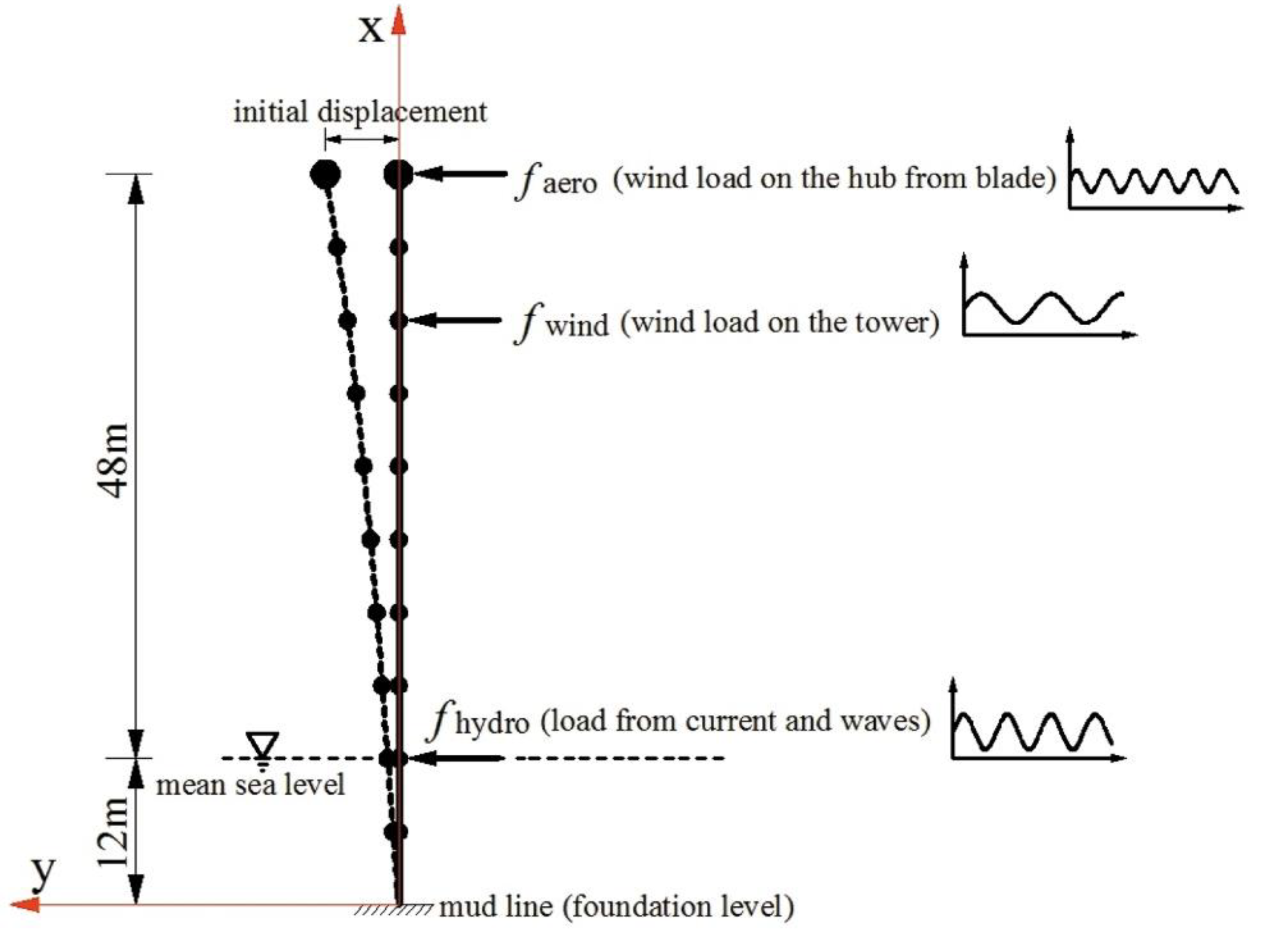
We chose the case of a monopile-supported wind turbine with a transient response as an example to verify the proposed method, as shown in Figure 1. The tower is modeled as a Euler–Bernoulli beam, with a concentrated mass set at the top of the tower to simulate the nacelle, hub, rotor blades, etc. The external diameter of the tower is 4 m with a wall thickness of 35 mm and a concentrated mass of 3.5 × 10⁵ kg. The elastic modulus is 2.05 × 10¹¹ N/m², and the mass density is 8450 kg/m³. The first two natural frequencies of the tower are f₁ = 1.0781 and f₂ = 6.7563 Hz, respectively.

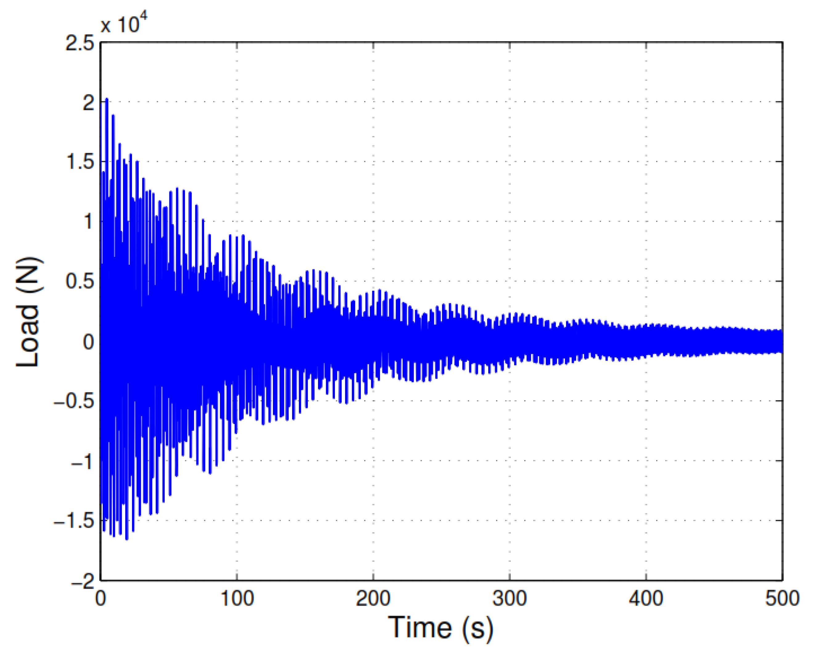
As described above, the theoretical purpose of the proposed method is to analyze the transient responses of the support structures caused by the heavy weight of the wind turbine. Therefore, the model damping should be obtained first. In this case, Rayleigh damping is selected in Figure 1 by $C=\alpha M+\beta K$ where $\alpha =\frac{4\pi f_1{f}_2}{f_1+f_2}\xi$ and $\beta =\frac{1}{\pi (f_1+f_2)}\xi$. Letting $\xi =0.3$ and substituting $f_1$ and $f_2$ into the above two equations, $\alpha$ = 0.3505 and $\beta$ = 0.0012 are obtained, respectively. Three types of loads are taken into account: the wind load on the hub from the blade ${\stackrel{⌢}{f}}_{aero}$, the wind load on the tower ${\stackrel{⌢}{f}}_{wind}$, and the wave load ${\stackrel{⌢}{f}}_{hydro}$. For simplification, the three types of loads are all simulated by the same formula:

$$f(t_k)={\displaystyle \sum _{n=1}^3{B}_n{e}^{{\xi }_n{t}_k}}\cos (2\pi f_n{t}_k+{\theta }_n)$$

(27)

The parameters in Equation (27) are shown in

Table 1. The parameters in Equation (29).

n	fn(Hz)	ζn	Bn(m)	θn(rad)
1	0.64	−0.003	40	−π/8
2	0.85	−0.01	100	−π/8
3	1.26	−0.01	80	π/6

. With the time interval ∆t = 0.1 s, the external load is shown in Figure 2 with a time period of 500 s.

3.1.1. Response Estimation of the Structure with Zero Initial Conditions

If the initial conditions are set to zero, the responses of the structure in the FD and TD can be estimated easily. Thus, the traditional FD methods and TD methods can be compared with the proposed method simultaneously. Implementing Equations (20) and (16), the eigenvalues ${\lambda }_n$ and the complex coefficients ${\epsilon }_n$ can be obtained, where n = 1, 2, 3:

$$\lambda =\left[\begin{array}{ccc}-0.0030\pm 4.0212i& -0.0030\pm 4.0212i& -0.0030\pm 4.0212i\\ -0.0100\pm 5.3407i& -0.0100\pm 5.3407i& -0.0100\pm 5.3407i\\ -0.0100\pm 7.9168i& -0.0100\pm 7.9168i& -0.0100\pm 7.9168i\end{array}\right]$$

(28)

and

$$\epsilon =\left[\begin{array}{ccc}1.8478\mp 0.7654i& 1.8478\mp 0.7654i& 1.8478\mp 0.7654i\\ 4.6194\pm 1.9134i& 4.6194\pm 1.9134i& 4.6194\pm 1.9134i\\ 3.4641\pm 2.0000i& 3.4641\pm 2.0000i& 3.4641\pm 2.0000i\end{array}\right]$$

(29)

After substituting Equations (28) and (29) into Equation (22) and then Equation (25), the discretized result without using DFT can be obtained by multiplying by a frequency interval $\delta f$ = 0.002 Hz. Because ${\stackrel{⌢}{f}}_{aero}$, ${\stackrel{⌢}{f}}_{wind}$, and ${\stackrel{⌢}{f}}_{hydro}$ are all simulated in Equation (27), the three types of loads share the same eigenvalues (Equation (26)) and complex coefficients (Equation (29)). Therefore, the structure responses can be estimated from the inverse Fourier transformation of Equation (26). Figure 3 shows the estimated response of the structure at the top of the tower in the y direction and the comparisons with the TD method and traditional FD method, respectively. From Figure 3, it can be concluded that the three methods agree well after a time of 5 s. The discrepancy between the TD and the FD method (0–5 s in Figure 3) comes from the fact that the traditional FD response is just the steady-state solution of Equation (6). Some differences in the estimated responses from 0 to 5 s can also be found between the proposed method and the TD method. This is due to the simplification of taking the real parts of the first complex number in Equation (25); a more detailed explanation can be found in Reference [15].

3.1.2. Free Response Estimation of the System

To consider the fact that the initial conditions at the start-up of the wind turbine should not be zero, three ideal scenarios were studied: (1) only the initial displacements have values while the initial velocities are zero, (2) only the initial velocities have values while the initial displacements are zero, and (3) a combination of both the displacements and velocities have values.

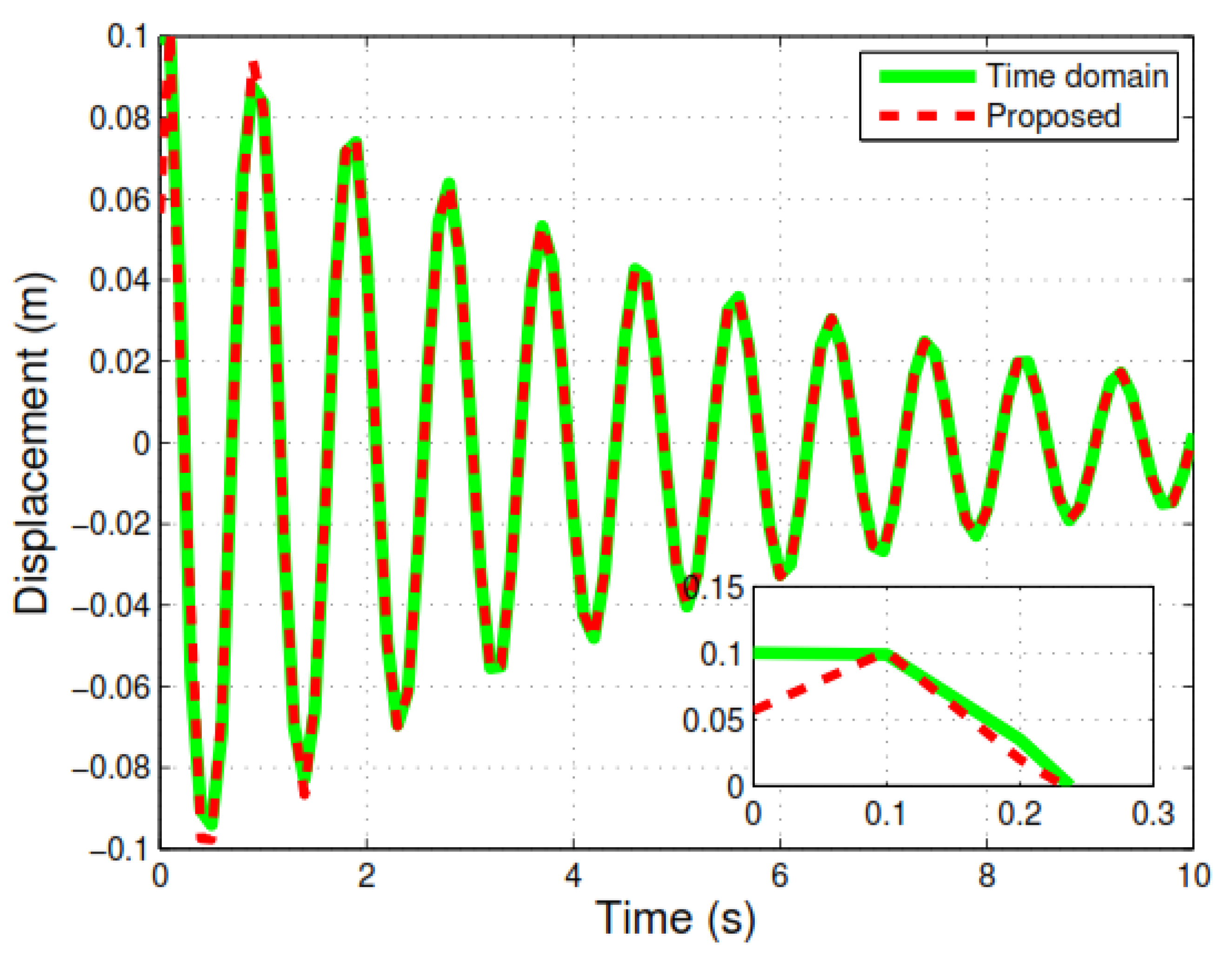
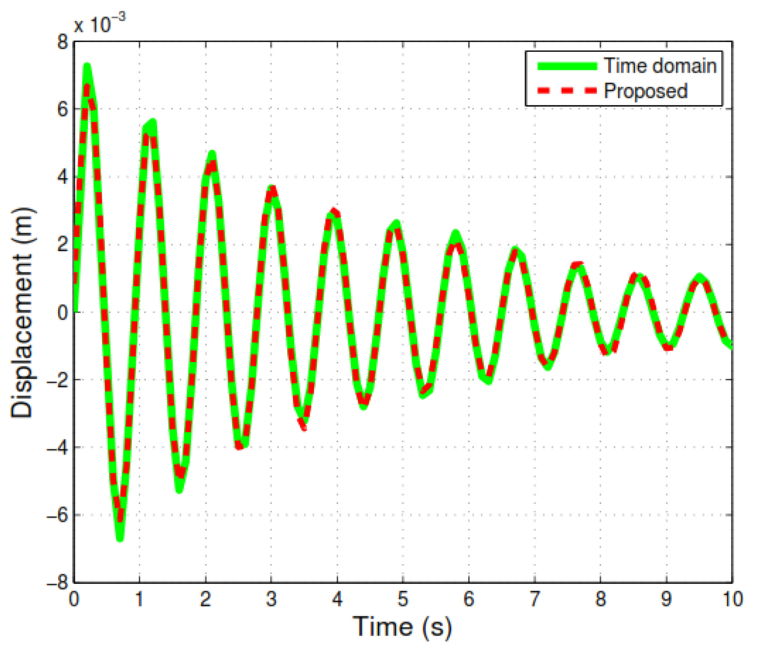
For the first scenario, we assume that the initial displacement at the top of the tower in the y direction is 0.1 m and that there is a linear decrease from the top to the bottom. To increase the computational efficiency, Equation (22) does not need to be calculated. Keeping δf = 0.002 Hz and implementing the inverse Fourier transformation of Equation (26), Figure 4 is obtained, which is the free response at the top of the tower in the y direction. It can be observed from Figure 4 that the responses of the tower with nonzero displacements can be obtained in the FD by using the proposed method and that the initial short-term discrepancy is unavoidable.

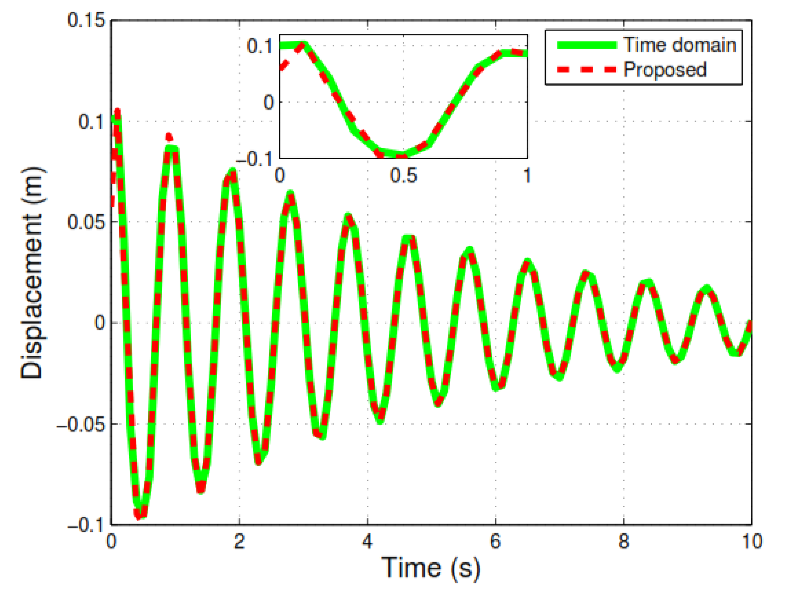
Similar to the first scenario, $\dot{\overline{x}}(0)$ = 0.25 m/s is applied to the top of the tower in the y direction in the second scenario. Figure 5 is a comparison of the estimated displacement corresponding to the same position in Figure 4, and it can be concluded that the results by the proposed method match well with those calculated by the TD method when only a nonzero velocity is applied.

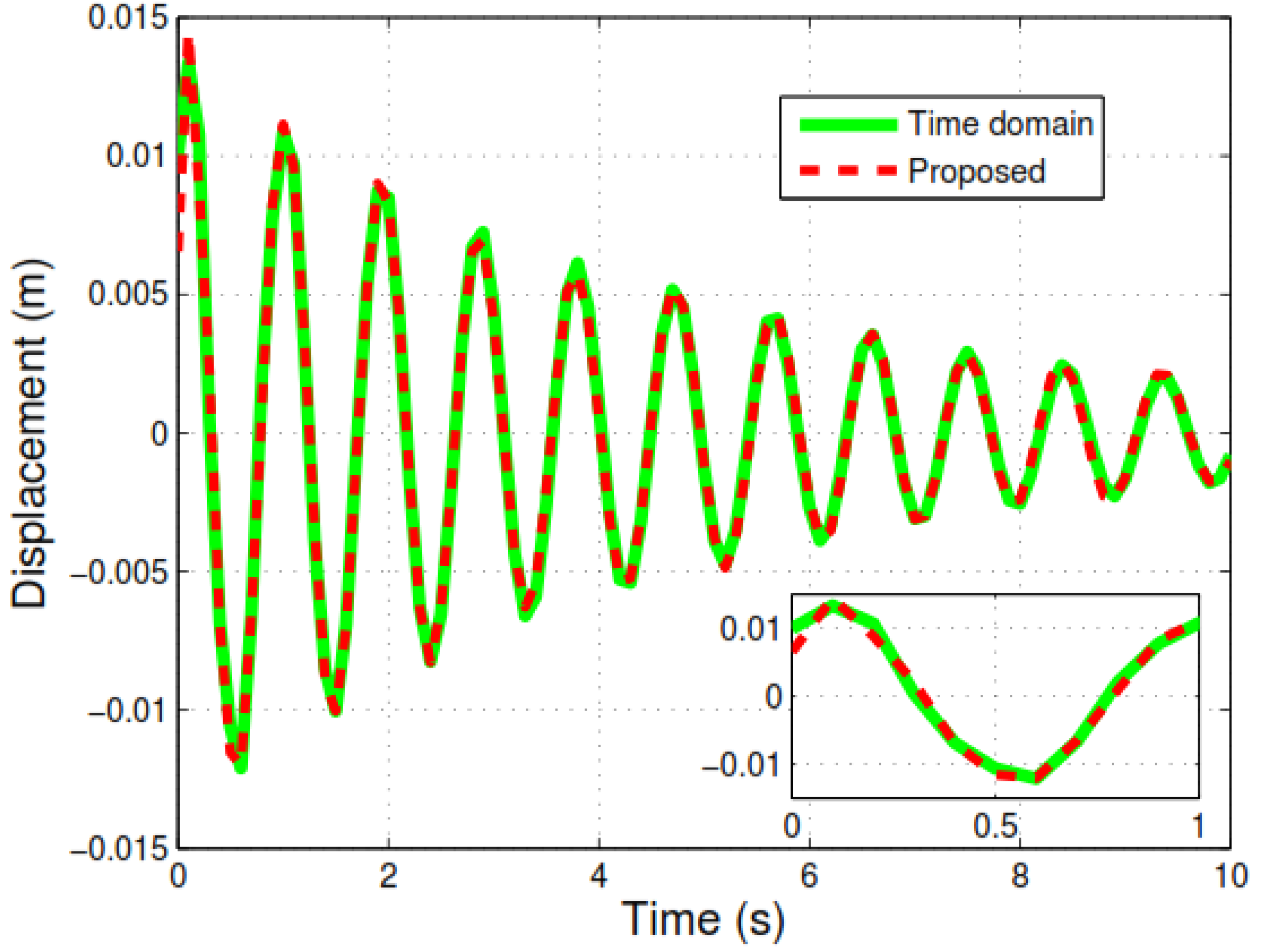
To ensure that the results from the three scenarios are comparable, the nonzero initial conditions used in Figure 4 and Figure 5 are adopted in the third scenario because it is a combination of the first two cases. Implementing the same procedure used in Figure 4 and Figure 5, the estimated response at the same position can be obtained, including a comparison with the results from the TD method, as shown in Figure 6. Figure 6 further demonstrates the accuracy and capability of the proposed method to address the problem of transient response estimation.

3.1.3. Response Estimation of the Structure with Nonzero Initial Conditions

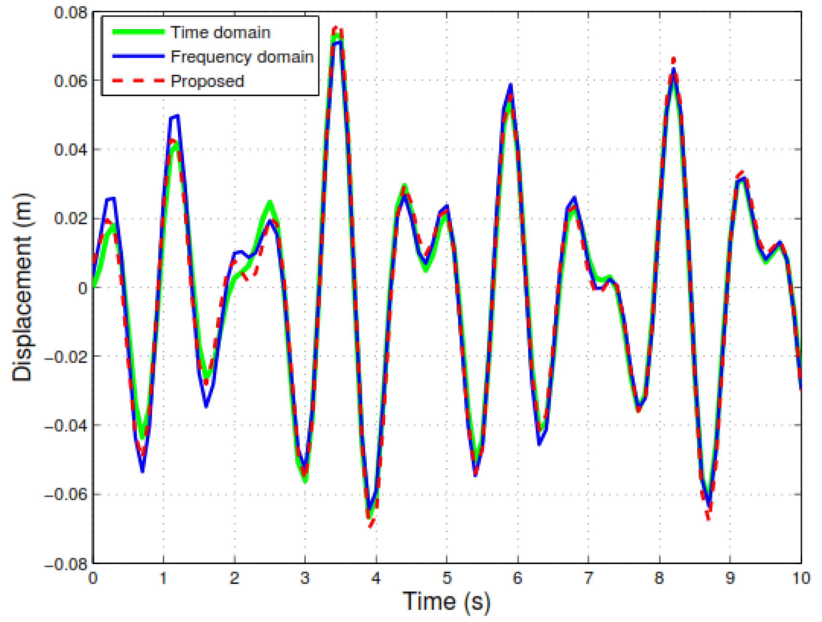
A general case is the response estimation of the structure subjected to all types of external loads, such as ${\stackrel{⌢}{f}}_{aero}$, ${\stackrel{⌢}{f}}_{wind}$, and ${\stackrel{⌢}{f}}_{hydro}$, and nonzero initial conditions $\overline{x}(0)$ and $\dot{\overline{x}}(0)$, which are taken into account simultaneously. To represent and simplify the general case, ${\stackrel{⌢}{f}}_{aero}$, ${\stackrel{⌢}{f}}_{wind}$, and ${\stackrel{⌢}{f}}_{hydro}$, generated by Equation (27), are applied to the positions as shown in Figure 1 and the nonzero conditions used in Figure 6 are maintained. By implementing the proposed method, Figure 7, which shows a comparison of estimated displacement using the TD method at the top of the tower in the y direction, is obtained. Figure 7 shows that the proposed method is capable of handling nonzero initial conditions in the FD and of estimating the responses of offshore wind turbine support structures.

3.2. A Jacket Support Offshore Wind Turbine

In the case of an offshore wind turbine with jacket support, two practical issues are discussed with respect to the application of the proposed method to a more sophisticated support structure, including the following: (1) Can the proposed approach address real measured or calculated external loads ${\stackrel{⌢}{f}}_{aero}$, ${\stackrel{⌢}{f}}_{wind}$, and ${\stackrel{⌢}{f}}_{hydro}$, and (2) How does the performance of the proposed method compare with that of commercial software (i.e., the accuracy or the computational efficiency of response estimation)?

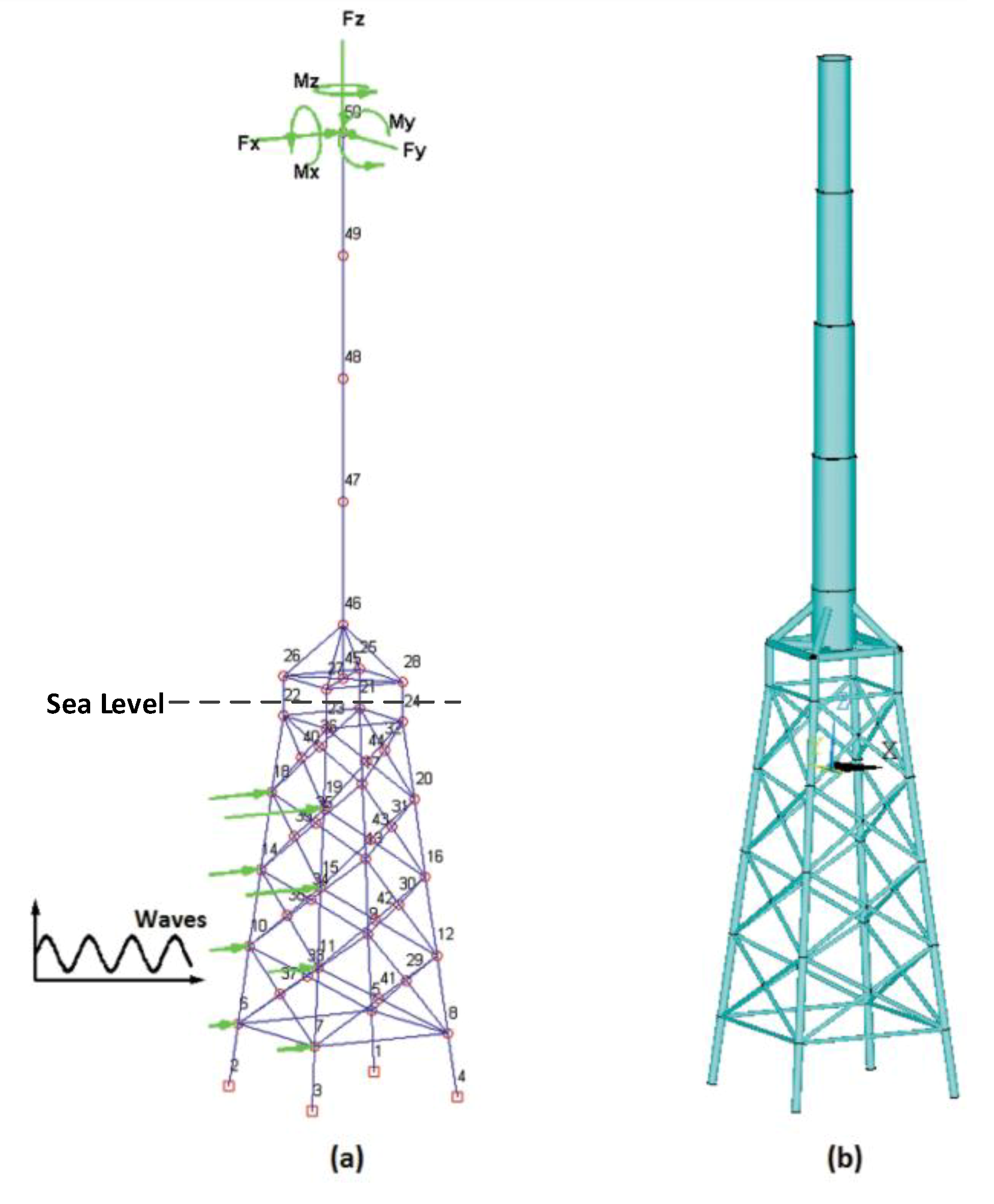
The jacket support structure, as shown in Figure 8, was also discussed in Reference [22]. The structure is located at a depth of 33 m in the water and includes the following components, among others: four battered legs (the incline is 9.9°), four central piles, and four levels of X-braces and mud braces. The height of the jacket substructure ranges from −33 m to 16.6 m above the mud surface level (MSL). The jacket connected to the tower bottom is about 16.6 m above the MSL, while the height of the upper tower is about 77.6 m. The base square area of the jacket is 21.536 m × 21.536 m, and the top square area is 12.323 m × 12.323 m. The cross section of the battered leg and X-braces and horizontal braces are 1.2192 m × 0.0254 m and 0.609 m × 0.0127 m, respectively. The bottom cross section and top cross section of the tower are 6.0 m × 0.06 m and 4.5 m × 0.055 m, respectively. The density of the steel used in the construction of both the tower and jacket is 8500 kg/m³. From an eigen analysis, the first two natural frequencies of the system are f₁ = 0.6503 and f₂ = 1.9979 Hz, respectively. In addition, Rayleigh damping is also taken into account, as in the first example.

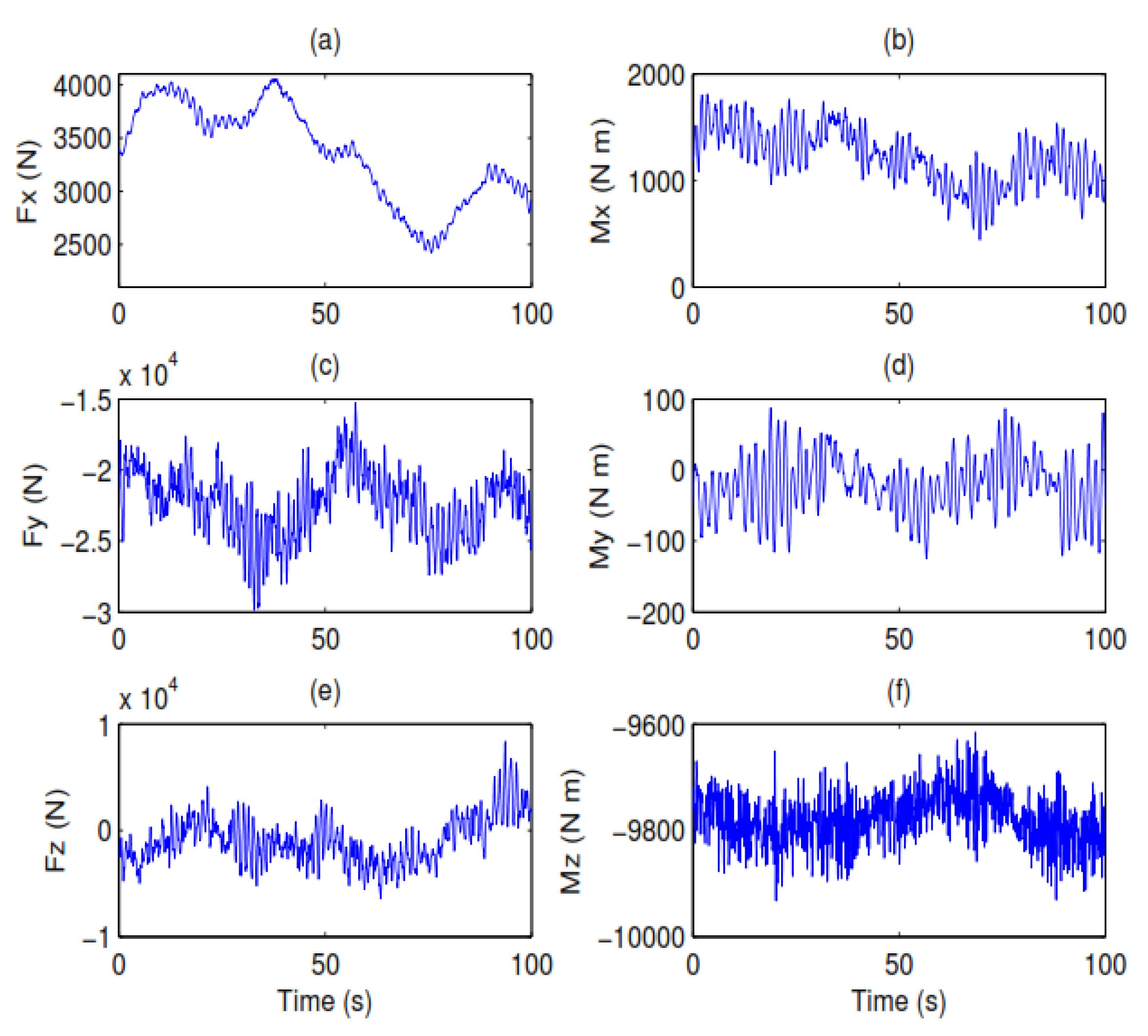
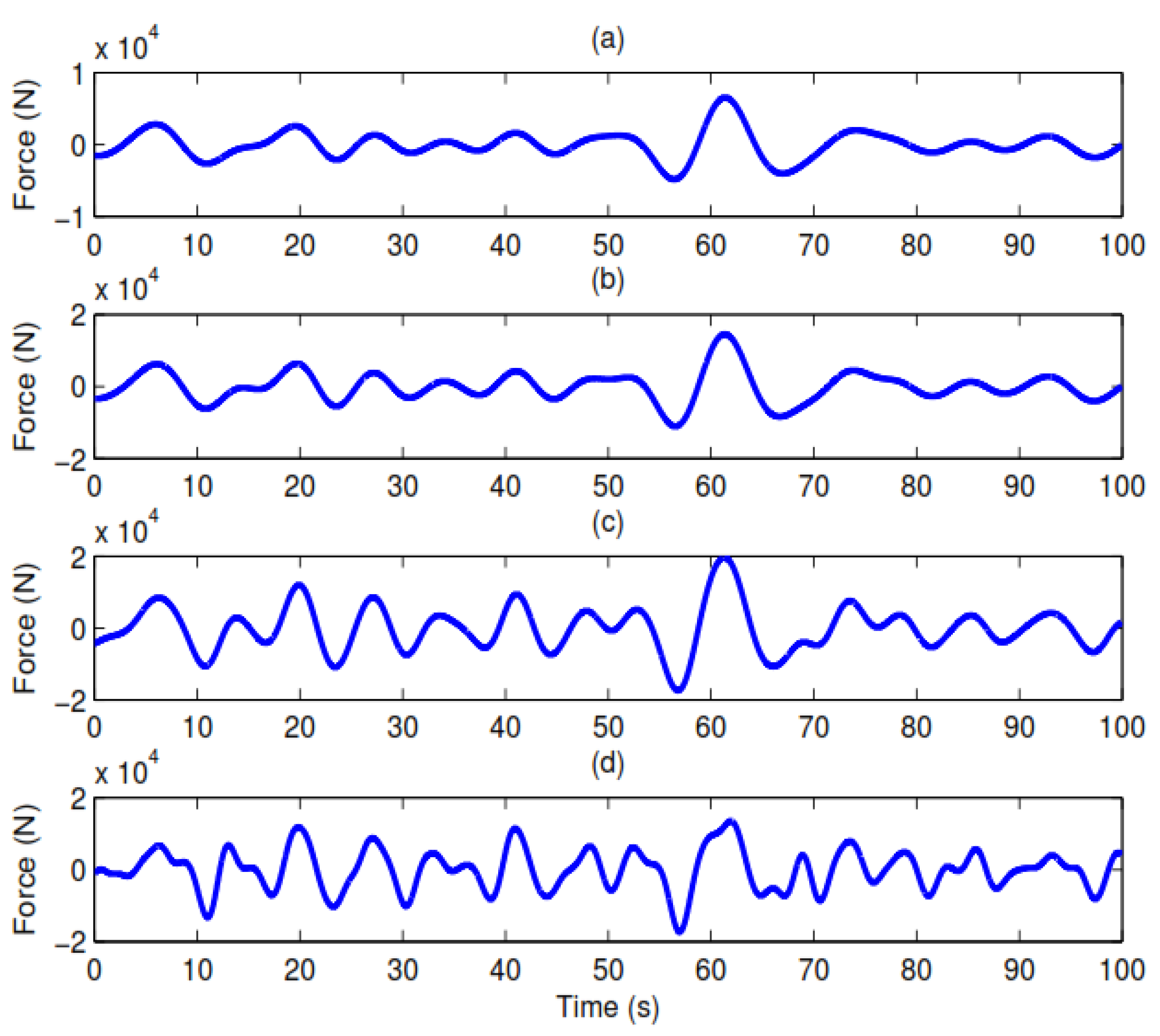
To solve the first issue, three forces and three moments, calculated by using commercial software, at the top of the tower were employed, as shown in Figure 9, which were applied to the six DOFs at node 50. The hydrodynamic loading, in terms of load per unit length for a given point in space and time, was calculated by using the Morison equation, and the free surface elevation timeseries was generated by discretizing the wave spectrum into a number of harmonic components with a constant frequency interval. For each discrete frequency, the corresponding harmonic wave amplitude was determined, and then, an irregular sea surface was obtained by assigning a random phase for each harmonic component; the detailed positions and corresponding timeseries of the imposed wave loads are shown in Figure 8 and Figure 10, respectively. The following sections are focused on the transient response estimation at any position of the structure.

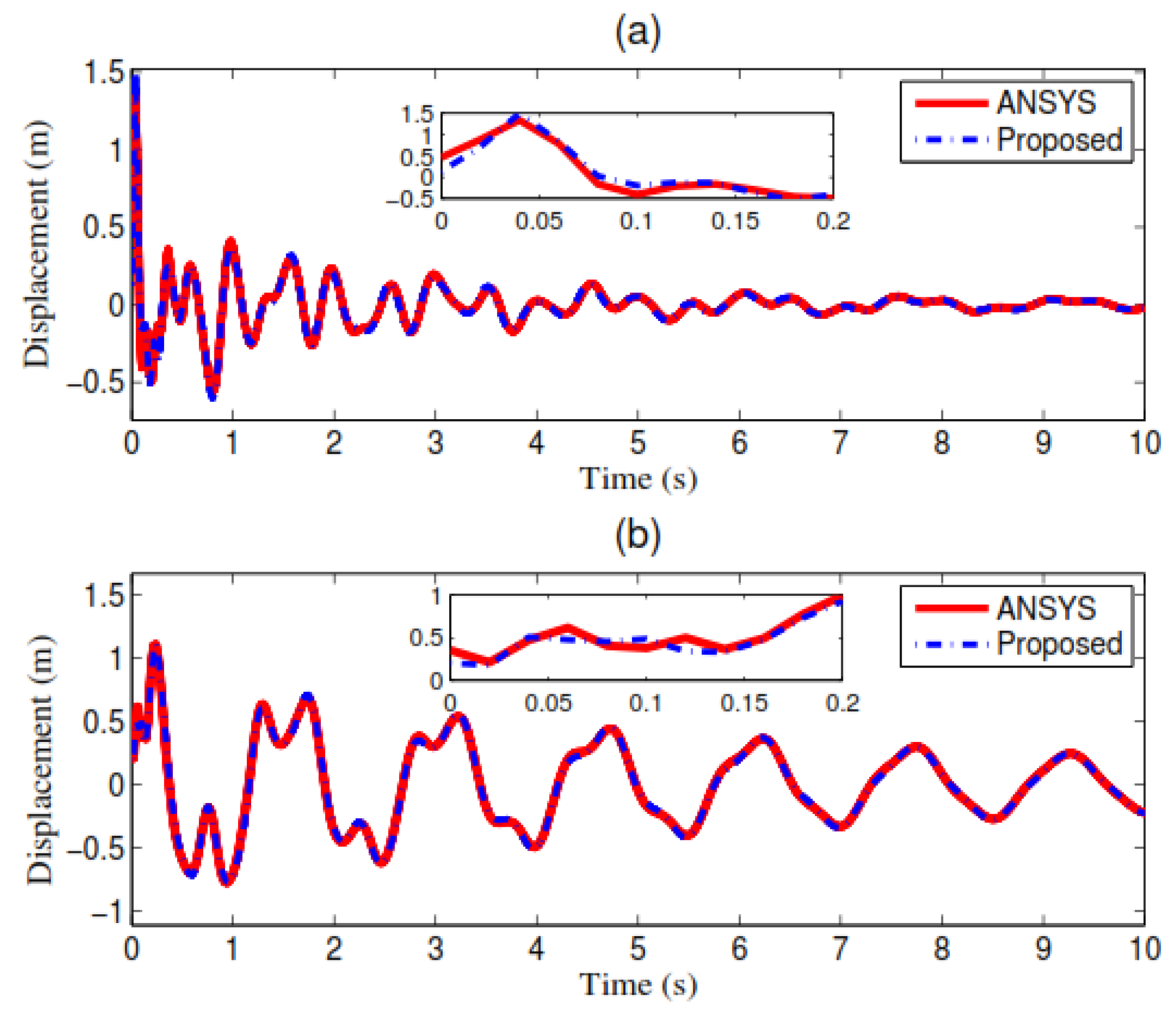
3.2.1. Response Estimation of the Structure with Partial Nonzero Initial Condition

A partial, nonzero initial condition is defined as a partial DOF of the structure, having a nonzero initial displacement and/or velocity. To consider the influence of wind turbine start-up or shutdown, we assumed that the tower has initial displacements at nodes 46–50 in the x direction changing from 0 to 0.2 m linearly and an initial velocity of 0.25 m/s added to node 50 in the x direction simultaneously. Comparing the calculation of eigenvalues ${\lambda }_n$ and the complex coefficients ${\epsilon }_n$ in this example with that from Equation (29), the model order for each load shown in Figure 9 is unknown and not constant for the six components of Figure 9. One possible way to address this issue is to set a different larger number for each timeseries and then to recheck the constructed load until it matches well with the remote signal in Figure 9 by adjusting the model order. The selected model orders for Mx, My, Mz, Fx, Fy, and Fz in Figure 9 are 240, 230, 370, 110, 280, and 300, respectively.

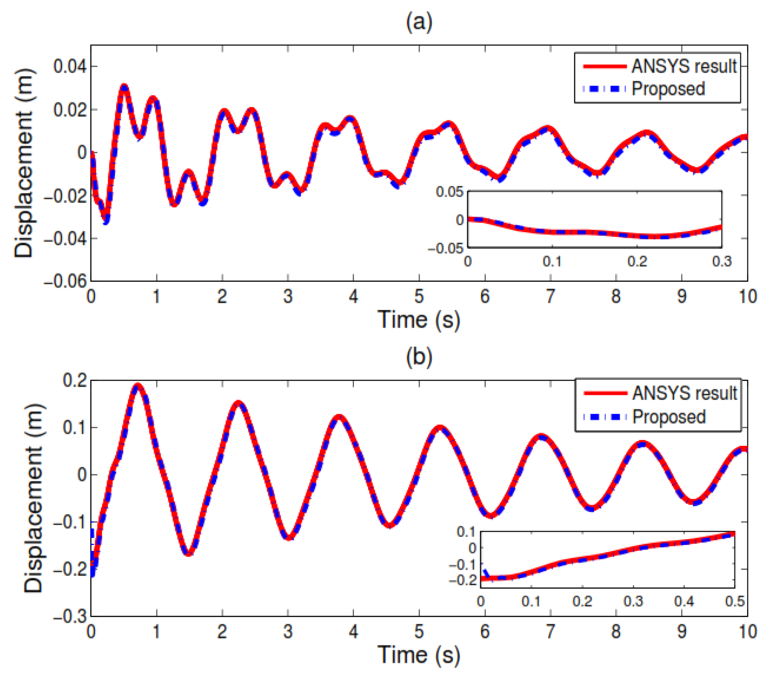
Similarly, all the eigenvalues and complex coefficients of the wave loads can be obtained by setting each model order to be 50. Substituting Equations (28) and (29) into Equation (22) and then Equation (25) and letting the frequency interval be $\delta f$ = 0.01 Hz, the responses can be estimated from the inverse Fourier transformation of Equation (26). Figure 11 shows a comparison of the estimated responses at nodes 28 and 50 in the x direction using the proposed method and ANSYS, respectively. Figure 11 clearly shows that the responses estimated by the proposed method match well with those by ANSYS, except for the initial part of the timeseries. The calculation process of Figure 11 also reveals that the central processing unit (CPU) time of the proposed method is mainly divided into two parts: (1) 624.35 s are dedicated to calculating the eigenvalues and complex coefficients altogether, i.e., 167.62 s for wave loads and 456.73 s for the six wind turbine loads, and (2) 97.22 s are used for transfer function and response estimation. The time step ∆t = 0.02 s is used for ANSYS, and 292 s are required for ANSYS’s response estimation, as shown in Figure 11. The transfer function calculation occupied most of the 97.22 s, which means that the computational efficiency of the proposed method will be improved if the transfer functions of the structure are pre-calculated and then reloaded into the response estimation when numerous scenarios are considered. Based on the above CPU time comparison, it could be expected that the proposed method will be as computationally efficient as the TD methods. However, the proposed method is actually more computationally efficient because Figure 11 only shows the results of 100 s, and the CPU time consumed by calculating the eigenvalues and complex coefficients for the three hours of external loads will not change significantly if these external loads meet the assumption of the time invariant, whereas the time for ANSYS will increase greatly because 5.4 × 10⁵ iterations will be required.

3.2.2. Response Estimation of the Structure with Universal Nonzero Initial Conditions

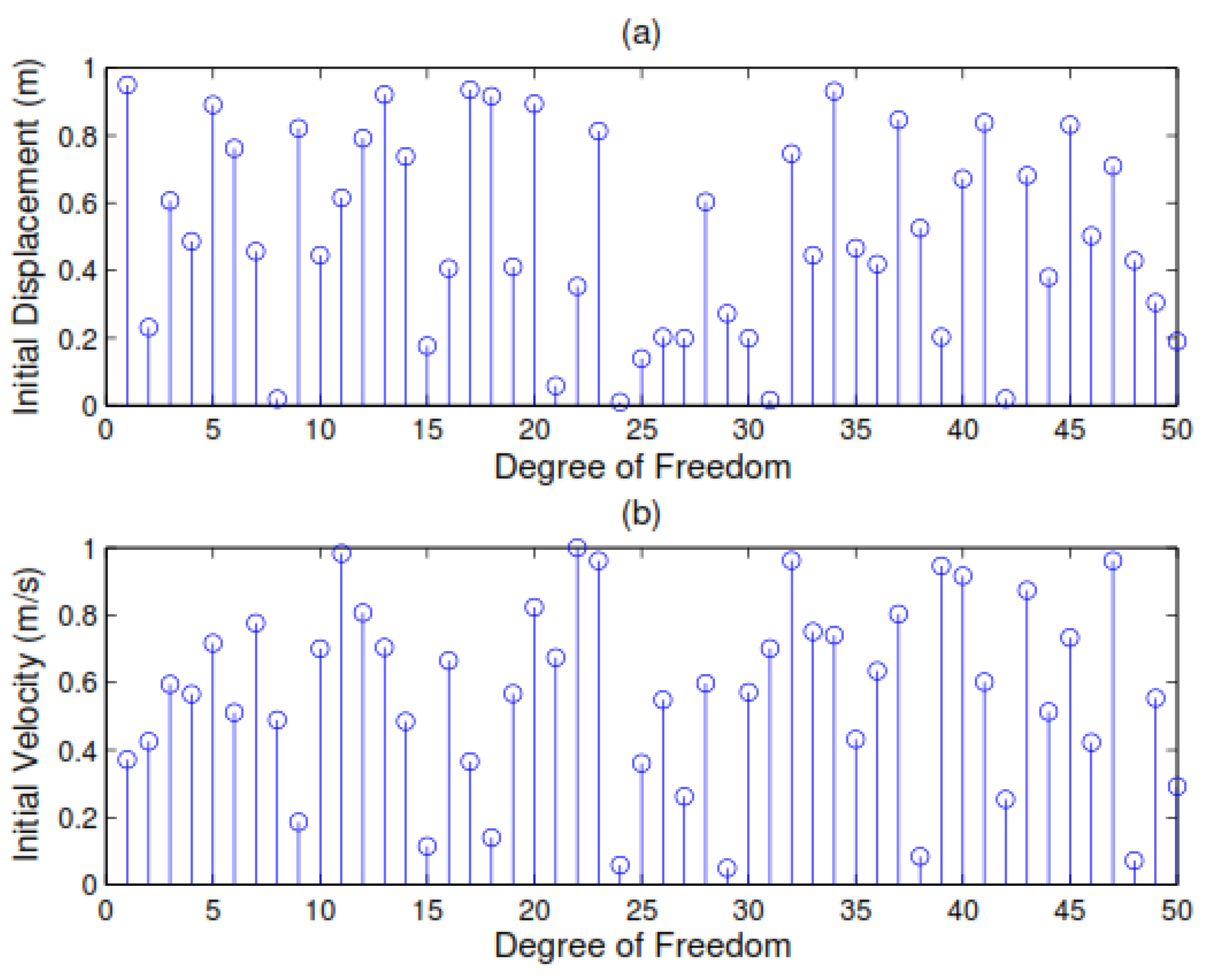
To demonstrate the robustness of the proposed method, another general case, defined as a universal state, in which there are nonzero initial conditions at each DOF of the structure, is presented here. Specifically, in the case of a universal state, the initial displacements and velocities are randomly generated, as shown in Figure 12 (only the former 50 values are plotted), and they are imposed on all the DOFs sequentially (1–276).

Implementing the proposed method, a comparison of the estimated responses with those from ANSYS is shown in Figure 13. Figure 13 shows that the randomly generated nonzero initial conditions could be considered and solved in the FD accurately by using the proposed method.

4. Conclusions

A novel transient response estimation method for offshore wind turbines in FD was presented in this paper. Any type of external load, such as wind turbine loads imposed at the top or bottom of the tower, winds, and waves, can be represented by its eigenvalues and corresponding complex coefficients and then easily combined with the initial displacement and velocity terms in the Laplace domain. Even though Fourier transform is not used in the FD to obtain expressions of external loads, the inverse Fourier transform (IFT) is employed in the proposed method to obtain responses in the TD. As DFT was not used, it can be concluded that the proposed method overcame the limitations of the periodic assumption of DFT. However, it should be noted that a small, earlier portion of the estimated responses contained errors because the simplification process takes the real part as the first complex number. Numerical results from a monopile-supported wind turbine with transient responses indicated that the approach matches well with the time-domain methods. The results of the second case study also indicate that the computational efficiency will be improved greatly if transfer functions of the structure are calculated previously and then reloaded into the procedure of the response estimation when thousands of scenarios are considered.

Currently, the proposed approach is limited to linear systems with symmetric mass, stiffness, and damping properties. Nonlinear problems and asymmetric damping will be studied in future research.

References

- Arany, L.; Bhattacharya, S.; Machdonald, J.H.G.; Hogan John, S. Closed form solution of Eigen frequency of monopile supported offshore wind turbines in deeper waters incorporating stiffness of substructure and SSI. Soil Dynam. Earthq. Eng. 2016, 83, 18–32. [Google Scholar] [CrossRef] [Green Version]
- Pérez-Collazo, C.; Greaves, D.; Lglesias, G. A review of combined wave and offshore wind energy. Renew. Sustain. Energy Rev. 2015, 42, 141–153. [Google Scholar] [CrossRef] [Green Version]
- Piersol, A.G.; Harris, C.M. Harri’s Shock and Vibration Handbook, 5th ed.; McGraw-Hill, Inc.: New York, NY, USA, 2017. [Google Scholar]
- Perez, T. Ship Motion Control: Course Keeping and Roll Reduction Using Rudder and Fins; Springer: London, UK, 2005. [Google Scholar]
- Hegseth, M.J.; Bachynski, E.E. A semi-analytical frequency domain model for efficient design evaluation of spar floating wind turbines. Mar. Struct. 2019, 64, 186–210. [Google Scholar] [CrossRef]
- Liu, F.S.; Lu, H.C.; Ji, C.Y. A general frequency-domain dynamic analysis algorithm for offshore structures with asymmetric matrices. Ocean Eng. 2016, 125, 272–284. [Google Scholar] [CrossRef]
- Liu, F.S.; Lu, H.C.; Li, H.J. Dynamic analysis of offshore structures with non-zero initial conditions in the frequency domain. J. Sound Vib. 2016, 366, 309–324. [Google Scholar] [CrossRef]
- Muk, C.O.; Bachynski, E.E.; Økland, O.D. Dynamic Responses of Jacket-Type Offshore Wind Turbines Using Decoupled and Coupled Models. J. Offshore Mech. Arctic Eng. 2017, 139, 041901. [Google Scholar]
- Seidel, M.; Ostermann, F.; Curvers, A.; Kuhn, M.; Kaufer, D.; Boker, C. Validation of offshore load simulations using measurement data from the DOWNVInD project. In Proceedings of the European Offshore Wind Conference, Stockholm, Sweden, 14–16 September 2009. [Google Scholar]
- Jia, J. An efficient nonlinear dynamic approach for calculating wave induced fatigue damage of offshore structures and its industrial applications for lifetime extension. Appl. Ocean Res. 2008, 30, 189–198. [Google Scholar] [CrossRef]
- Chen, I.W.; Wong BL Lin, Y.H. Design and analysis of jacket substructures for offshore wind turbines. Energies 2016, 9, 264. [Google Scholar] [CrossRef]
- Dong, W.B.; Moan, T.; Gao, Z. Long-term fatigue analysis of multi-planar tubular joints for jacket-type offshore wind turbine in time domain. Eng. Struct. 2011, 33, 2002–2014. [Google Scholar] [CrossRef]
- Anders, E.Z. Understanding FFT Second Edition Extensivel Y Revised Applications; Citrus Press: Titusville, FL, USA, 2004. [Google Scholar]
- Newman, J. Marine Hydrodynamics; MIT Press: Cambridge, MA, USA, 1977. [Google Scholar]
- Faltinsen, O. Hydrodynamic of High-Speed Marine Vehicles; Cambridge University Press: Cambridge, UK, 2006. [Google Scholar]
- Liu, F.S.; Li, H.J.; Wang, W.Y.; Liang, B.C. Initial-condition consideration by transferring and loading reconstruction for the dynamic analysis of linear structures in the frequency domain. J. Sound Vib. 2015, 336, 164–178. [Google Scholar] [CrossRef]
- Support Structures for Wind Turbines; Offshore Standard, DNVGL- ST-0126; DNVGL: Akershus, Noway, 2018.
- Environmental Conditions and Environmental Loads; Recommended Practice, DNV-RP-C205; DNVGL: Akershus, Noway, 2007.
- Kim, J.H.; Kim, Y.H. A predictor-corrector method for structural nonlinear analysis. Comput. Methods Appl. Mech. Eng. 2001, 191, 959–974. [Google Scholar] [CrossRef]
- Erwin, K. Advanced Engineering Mathematics, 8th ed.; John Wiley & Sons, Inc.: New York, NY, USA, 1999. [Google Scholar]
- Golub, G.H. Matrix Computations, 3rd ed.; Johns Hopkins University Press: Baltimore, MD, USA, 1996. [Google Scholar]
- Shi, W.; Park, H.; Han, J.; Na, S.; Kim, C.W. A study on the effect of different modeling parameters on the dynamic response of a jacket-type offshore wind turbine in the Korean Southwest Sea. Renew. Energy 2013, 58, 50–59. [Google Scholar] [CrossRef]
Figure 1.
A sketch of a monopile-supported wind turbine.
Figure 2.
The external load of the monopile-supported wind turbine.
Figure 3.
The response comparison at the top of the tower in the y direction with a zero initial condition when an external load is applied.
Figure 4.
The response comparison at the top of the tower in the y direction when only nonzero displacements are applied.
Figure 5.
The response comparison at the top of the tower in the y direction when only a nonzero velocity is applied.
Figure 6.
The response comparisons at the top of the tower in the y direction when nonzero displacements and velocity are applied simultaneously.
Figure 7.
The response comparison at the top of tower in the y direction when external loads, nonzero displacements, and velocity are applied simultaneously.
Figure 8.
A sketch of a jacket support offshore wind turbine: (a) the MATLAB model and (b) the ANSYS model.
Figure 9.
The equivalent loads converted to the top of the tower caused by the wind turbine: (a) Fx, (b) Mx, (c) Fy, (d) My, (e) Fz, and (f) Mz.
Figure 10.
The wave loads at different elevations: (a) −33 m, (b) −22 m, (c) −11 m, and (d) 0 m.
Figure 11.
The response comparisons with ANSYS at nodes 28 and 50 in the x direction: (a) node 28 and (b) node 50.
Figure 12.
The randomly generated initial conditions: (a) initial displacement and (b) initial velocity.
Figure 13.
The response comparisons with ANSYS at nodes 28 and 50 in the x direction: (a) node 28 and (b) node 50 using random initial conditions.