An Evolutionary Computational Approach for Designing Micro Hydro Power Plants


Departamento de Ingeniería, Universidad Loyola Andalucía, 41014 Seville, Spain
*
Author to whom correspondence should be addressed.
Energies 2019, 12(5), 878; https://doi.org/10.3390/en12050878
Submission received: 27 December 2018
/
Revised: 7 February 2019
/
Accepted: 19 February 2019
/
Published: 6 March 2019
Abstract
:Micro Hydro Power Plants (MHPP) constitute an effective, environmentally-friendly solution to deal with energy poverty in rural isolated areas, being the most extended renewable technology in this field. Nevertheless, the context of poverty and lack of qualified manpower usually lead to a poor usage of the resources, due to the use of thumb rules and user experience to design the layout of the plants, which conditions the performance. For this reason, the development of robust and efficient optimization strategies are particularly relevant in this field. This paper proposes a Genetic Algorithm (GA) to address the problem of finding the optimal layout for an MHPP based on real scenario data, obtained by means of a set of experimental topographic measurements. With this end in view, a model of the plant is first developed, in terms of which the optimization problem is formulated with the constraints of minimal generated power and maximum use of flow, together with the practical feasibility of the layout to the measured terrain. The problem is formulated in both single-objective (minimization of the cost) and multi-objective (minimization of the cost and maximization of the generated power) modes, the Pareto dominance being studied in this last case. The algorithm is first applied to an example scenario to illustrate its performance and compared with a reference Branch and Bound Algorithm (BBA) linear approach, reaching reductions of more than 70% in the cost of the MHPP. Finally, it is also applied to a real set of geographical data to validate its robustness against irregular, poorly sampled domains.
Keywords:
MHPP; hydro-power; penstock; optimization; GA; simulated annealing; evolutionary computation1. Introduction
The increasing rate of energy demand around the world represents one of the biggest challenges that humanity has to face in the future [1]. Although population growth and increasing industrialization are the main reasons, the expansion of global access to electricity plays a relevant role. According to the World Data Bank [2], approximately 1.1 billion people lacked access to electricity in 2014, representing 15% of the world population. While urban areas tend to be more electrified, rural areas are the most affected by the lack of access to electricity. The population without electricity in these areas represents 27% of the total, in comparison with the 4% of urban populations with the same problem. Furthermore, these statistics are more critical in developing countries. Given this, the expansion of electricity supply represents an area of interest in these countries [3], which tend to include rural electrification programs in order to improve life quality of the rural population.
In this context, Renewable Energy Sources (RES) play a fundamental role [4], becoming an effective way to guarantee the increasing need of energy supply (some works conclude that by 2050 renewables could provide half of the world’s energy needs without affecting the climate system [5]) without compromising the natural resources while mitigating CO2 emissions. Although different options have been demonstrated to be adequate to promote the reduction of greenhouse gas (GHG) emissions, such as nuclear energy or carbon capture and storage (CCS), the use of RES is praised as one of the most suitable options [6]. These sources are carbon-free (with a few exceptions, such as certain bioenergy production methods and bioenergy life-cycle), and their resource potential does not deplete over time, in contrast with the limitations of nuclear and fossil fuel availability. The major disadvantages of RES systems are fundamentally related to the uncertainty implied by the stochastic nature of the natural sources, which translates into a limitation to high levels of electricity production [7]. Nevertheless, these limitations have no important effects on small generation systems, which makes RES ideal candidates meet the energy supply requirements in remote, isolated areas [8,9], where national grids are not accessible due to geographical or economic reasons.
Although several alternatives have been demonstrated to be suitable to supply electric power to remote isolated areas [10,11,12], hydropower has established itself as the most frequently used around the world [13], with the highest efficiency rates [14]. Given its versatility and stable projection [15], hydropower plants represent an effective, suitable option for the supply of rural isolated areas [16], being also the cheapest option for off-grid generation [17].
Notwithstanding this, the context of these locations constitute a challenge for the optimal design of hydro plants among others. The lack of qualified manpower and the limitation of the resources are barriers to the optimal development of these installations. Within this framework, the study of efficient design strategies is essential to guarantee that the resources are used in the most efficient way, without compromising the limited resources.
1.1. Micro-Hydro Power Plants
Micro-Hydro Power Plants (MHPPs) are defined as hydro power stations with generation capacities of up to 100 kW [18]. These installations require relatively small power sources and are suitable to supply small communities through an independent electrical grid [19]. Generally, the only requisites for an MHPP are a stream with a certain flow rate that satisfies a height difference. Unlike big hydro installations, where the design implies advanced architectures, such as large civil works, surge tanks, multiple generation units or the use of advanced regulating equipment, MHPP are simple and robust installations with minimal equipment and labor requirements. In a basic MHPP, the water is directly extracted from the natural course, without the need for establishing a water reservoir. Although a small dam is generally built, its purpose is to guarantee a smooth and clean entrance of the water to the penstock. The penstock is a long pipe that drives the water downhill and leads into a powerhouse, a small civil construction where the generation equipment (turbine and generator) is installed (see the scheme in Figure 1). Inside the powerhouse, the water flow is driven into the turbine, where the energy of the water flow is transformed into mechanical. This last is converted into electrical energy through a generator, to which the turbine axis is connected. After the energy conversion, the water is returned back to its natural course.
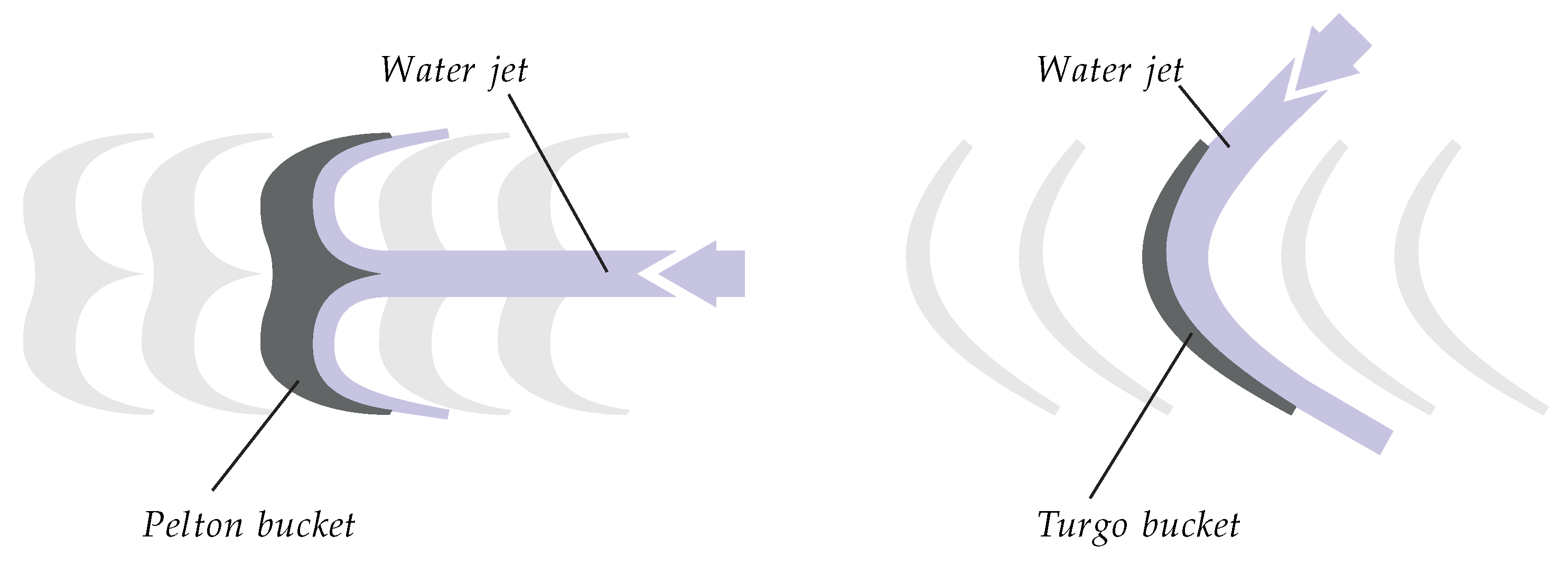
Although non-traditional alternatives are frequently used as a turbine, such as locally made systems or pumps working as turbines (PAT) [20], Pelton and Turgo wheels are the usual choices, given their suitability to high height and low flow rates emplacements [21]. Pelton and Turgo wheels are action turbines, that is, the energy of the water flow is fully converted into kinetic before its transformation into mechanical energy. This is done by the formation of a water jet through an injector. This water jet is projected to the buckets, which are disposed circumferentially around the wheel (see Figure 2), generating a net torque which moves the turbine.
1.2. Traditional Design Procedure of MHPPs in Rural Emplacements
The design of an MHPP is generally divided into the following steps:
- Measurement of available flow rate, Q.
- Measurement of available height, .
- Decision-making of dam and powerhouse location.
- Estimation of power generation, P.
- Sizing of the equipment.
The measurement of the available flow rate and height constitutes the evaluation of the emplacement, and is focused on evaluating the potential of the water resource. As flow data records are not usually available for small rivers and streams, in situ measurements are generally needed. Several methods are available for this purpose, the use of gauging weirs [22] being the most common. After the available flow rate has been evaluated, the gross height is estimated either by using traditional methods, such as height maps or Topographic Abney levels, or more sophisticated methods such as digital altimeters or GPS, according to equipment availability. Once the water flow and height have been estimated, the location of the dam and the powerhouse are chosen by the hydro power professionals on the basis of an initial site visit and know-how. This decision is focused on minimizing the pipe length, L, as this variable will strongly condition the cost and the final performance of the MHPP. After this decision is made, an estimation of the generated power can be made using
Q being the water flow rate, the gross height, the specific weight of water, g the gravity acceleration and an average efficiency of the generation equipment (turbine and generator). This estimation represents the assumption of considering as the total height at the disposal of the turbine. As it will be described later, the friction loss through the penstock implies that the actual net head at the turbine, named h, is lower than . In addition to this, the transformation of this potential energy into electrical energy has a certain efficiency that leads to an additional decrease of the generated power. Nevertheless, expression (1) is useful for a rough estimation of the potential in a certain emplacement. Based on this, the generation system (pipe, turbine and generator) can be sized using thumb rules [23].
Althogh this traditional methodology constitutes an economic, robust strategy of design for MHPP, it is relevant to note that several aspects of it can be improved in order to make a better utilisation of the resources without compromising either the benefits of the methodology or its simplicity. On this basis, this work proposes the use of an evolutionary computational approach to assist the design of the MHPP layout.
Contributions
This work presents the application of evolutionary computational methods to address the problem of finding the most suitable layout for an MHPP. Although the optimization of MHPP to supply remote areas has been extensively approached in the literature [24,25,26,27], most of the studies aim at developing general guidelines, while the study of particular design strategies to assist the implementation of MHPP considering the real scenario characteristics is still a matter of study. In addition, the nonlinear nature of the performance of an MHPP in a particular location represents a complexity that has generally been addressed by either simplifications of the domain (approximating the river profile by a straight line [28]), or simplifying the problem (fixing certain parameters, such as the pipe diameter [29]). Although the existing strategies lead to a better usage of the resources, the simplifications imply that the obtained solutions may differ from the optimal solutions of the real problem. In this paper, the use of genetic algorithms (GA) is proposed to determine the most suitable layout of an MHPP for a real scenario, the terrain profile being obtained by means of a topographic survey, and considering a complete model of the plant. The paper aims to find the most suitable location of the powerhouse and the dam, together with the distribution of pipe lengths that best suit the terrain profile, including the selection of the most adequate penstock diameter, according to a set of performance criteria. In addition, to obtain a deeper and more detailed analysis, the multi-objective problem is studied and two competitive objectives of the model are optimized, providing a better understanding of the design variables range and the influence of the different parameters in the performance of the MHPP. An example river profile scenario is first used to evaluate the effectiveness of the proposed approach, being also a real scenario profile used to test its robustness with irregular sampling.
This paper is organized as follows: In Section 2, an introduction to related work in the literature is presented, where the advantages of the proposed approach are presented. In Section 3, a general overview of the problem set-up and its main variables are detailed. In order to do that, a model of an MHPP is first developed in terms of the decision variables, and then this model is used to define the problem of optimally designing the MHPP layout. In Section 4, an evolutionary computational approach is developed to address the optimization problem, this approach being used in an example problem. Finally, an analysis of the results, together with an additional application of the algorithm to a real scenario and the concluding remarks are summarized in Section 5.
2. Related Work
The problem of finding optimal parameters to design small and micro hydro power plants has motivated extensive studies in the literature [30,31,32,33,34,35,36]. Given the complexity that this problem has shown since the first studies [30], heuristic approaches are exhibing a particular relevance in this field [31], not just to assist the design of the plants but also to optimize the management and operation strategies. This is due to the complexity of approaching these problems analytically, due to the high number of variables, nonlinearities and other complexities, therefore strong simplifications are generally made, the optimal power capacity being the usual objective function. A relevant work in optimal design of small hydro power systems is [27], where authors propose the sizing of the plants by using an evolutionary algorithm that assumes the stochastic nature of the water resource, in the single and two-objective modes. This way, authors are able to identify the most advantageous design alternatives for a project. In a similar way, dynamic programming was used in [32] to evaluate the effects of the parameters by means of a sensitivity analysis approach. In addition, in [26], a cost optimization is proposed by using a Honey Bee Mating Optimization (HBMO) algorithm [37]. Furthermore, several authors have proposed different tools to assist the development of new optimization strategies, such as methods to determine the turbine configuration [33] and the cost of the plant [34].
Regarding analytical approaches, several techniques, based on traditional methods (such as mix-integer programming, quadratic programming, Lagrangian relaxation, etc), have been proposed [35,36]. In [38], the authors propose an analytical framework based on a description of the plant capacity that maximizes the energy in terms of the flow duration curves. In a similar way, in [39], a linear programming model is presented to maximize the generation of a hydro power plant using collected data from a real plant in Korea. Similar optimization strategies can also be found in the literature to solve other problems related to hydraulic energy that share a similar nature with the roblem studied in this paper [40,41,42]. For example, in [40], authors propose a mixed-integer nonlinear programming approach to address a water-network optimization problem, showing good results on complex real-world instances. Although these works can provide general guidelines to assist the design of MHPPs, there is still a lack of knowledge regarding the in situ development of these plants, where the limitations of the resources make the design of the plant extremely sensitive to design parameters, encouraging the develop of practical techniques to guarantee that the resources are used in the most efficient way. Following this line of work, authors in [28,43] study the most cost-effective penstocks, proposing a set of modular systems. Similarly, Ref. [44] proposes an approach to determine the optimal discharge and penstock diameter in terms of the characteristics of the MHPP. This draws from the premise of a constant slope, which is a severe idealization of the real river profile. Although for long penstocks this approximation can be reasonable, for the general case of small penstocks in MHPPs, the influence of the real river profile is significant, and its consideration can condition the performance of the designed MHPP. Following this, in [29], an example river profile is considered, by means of a topographic survey, and an optimization problem to find the optimal layout of an MHPP is formulated. Although the results exhibit a good performance of the proposed approach, the requirement of a linear formulation implies that the penstock diameter is fixed, as its effects on the performance (through the hydraulic loss) is strongly nonlinear. This represents an important drawback, as introducing the pipe diameter as a design variable clearly leads to better solutions.
In this work, an evolutionary computational approach is proposed to address the problem presented in [29]. Taking advantage of the search power of this approach in combinational optimization problems, the design is improved by incorporating the diameter of the penstock as a decision variable, so better and more efficient solutions can be obtained. Additionally, the problem is formulated as multi-objective optimization based on Pareto dominance, so the minimization of the cost and the maximization of the power generation are considered simultaneously, the Pareto front being obtained and studied in depth.
3. Problem Statement
The problem of finding the most suitable layout is of great importance in the design of MHPP, as it strongly conditions its performance. An appropiate design requires finding a compromise between a high gross height and a low need of pipe and civil work. A high gross height provides a big potential energy to be used, but a long penstock can have negative effects on its usage, as the friction losses grow, especially for low penstock diameters [45]. To provide a base to develop optimization strategies, a realistic model of an MHPP is first developed in this section, the optimization problem then being formulated.
3.1. Model of the System
The model of the MHPP is formulated through the gross head and the water flow rate Q, in terms of which the rest of relevant design variables can be defined. These variables are the power generated, P, and the cost of the plant, C.
3.1.1. Generated Power
The true obtainable power, P, of an MHPP can be expressed as
where h, as explained previously, represents the net height at the entrance of the turbine. This net head differs from the gross height, , by means of the friction loss along the penstock, due to the non-ideal behavior or the inner walls of the pipes. Using to refer this loss, it can be written as
Note that the expression in Label (1) represents a simplification of Label (2), where the loss in the penstock, , has not been taken into consideration. Assuming the typical case of an action turbine, the water height at the entrance of the turbine, h, is entirely kinetic, so it can be expressed in terms of the velocity of the jet, , as
where, due to incompressibility of water, this last variable, , can be expressed in terms of the flow, Q, and the sectional area of the nozzle injector :
where the coefficient of discharge has been introduced to model the formation of a vena contracta after the water leaves the nozzle [23]. Using this last expression, the height at the entrance of the turbine, h, can be written in terms of the flow as
In addition, the losses through the penstock can be approximated as in [29], yielding that
being a constant that depends on the pipe material, and and L its diameter and length, respectively. Introducing expression (4) in (5), and the resultant expression, together with (6), in (3), it yields that
Finally, introducing (6) and (5) in (2), together with (7), an expression of the generated power, P, in terms of the main variables, and L, is obtained as
It is worth pointing out that the power generated by an MHPP is determined by the water flow Q, the gross height , and the penstock length and diameter, L and . These variables are clearly defined and have a direct interpretation in terms of the design of an MHPP layout. For this reason, they are considered as design variables for the plant in this work. Following this, the problem will be formulated in such way that each solution defines a set of these variables, so the performance of the MHPP, and, thus, the fitness of the solution, can be easily evaluated.
3.1.2. Cost Function
The cost of the installation represents a strong limitation for the success of the project, given the context of precariousness presented in Section 1. Therefore, it is a variable that must be considered. It is relevant to note that the overall cost of the installation includes not just the penstock, the dam, and the powerhouse, but also the turbine and the generator. Nevertheless, the sizing of the generator is generally conditioned by the order of the power estimation at each location, as the device selection is made for a wide margin of nominal operation points. With respect to the turbine, given the estimation of the flow rate and power, its dependency on the nominal point does not present a significant difference in the manufacturing process, as the cost is approximately the same if slightly geometric variances are made to the design. For these reasons, the location of the dam and the powerhouse, together with the layout of the penstock represent the main conditioning factors with regard to the optimization of the funding resources. The cost of the generating equipment is then considered constant in this work, and thus can be ignored in the optimization problem.
The price of a piping installation typically varies linearly with the total length of the pipe, L, and the squared diameter, [28]. Furthermore, although the pipe length and the number of pipe connections do not affect directly the cost, an excessive amount of them may imply the unfeasibility of a solution due to the difficulties associated with the civil work. For this reason, it is usually recommended to moderate their use. For this reason, following [29], a constant is introduced to model the equivalent cost (in pipe length) of installing an elbow between two straight pipe lengths, so the implications of the number of elbows, , can be considered in the cost. With all this, the cost of the penstock can be expressed as
being an arbitrary constant to express the cost in the appropiate units and magnitude.
3.1.3. Model of the MHPP Layout
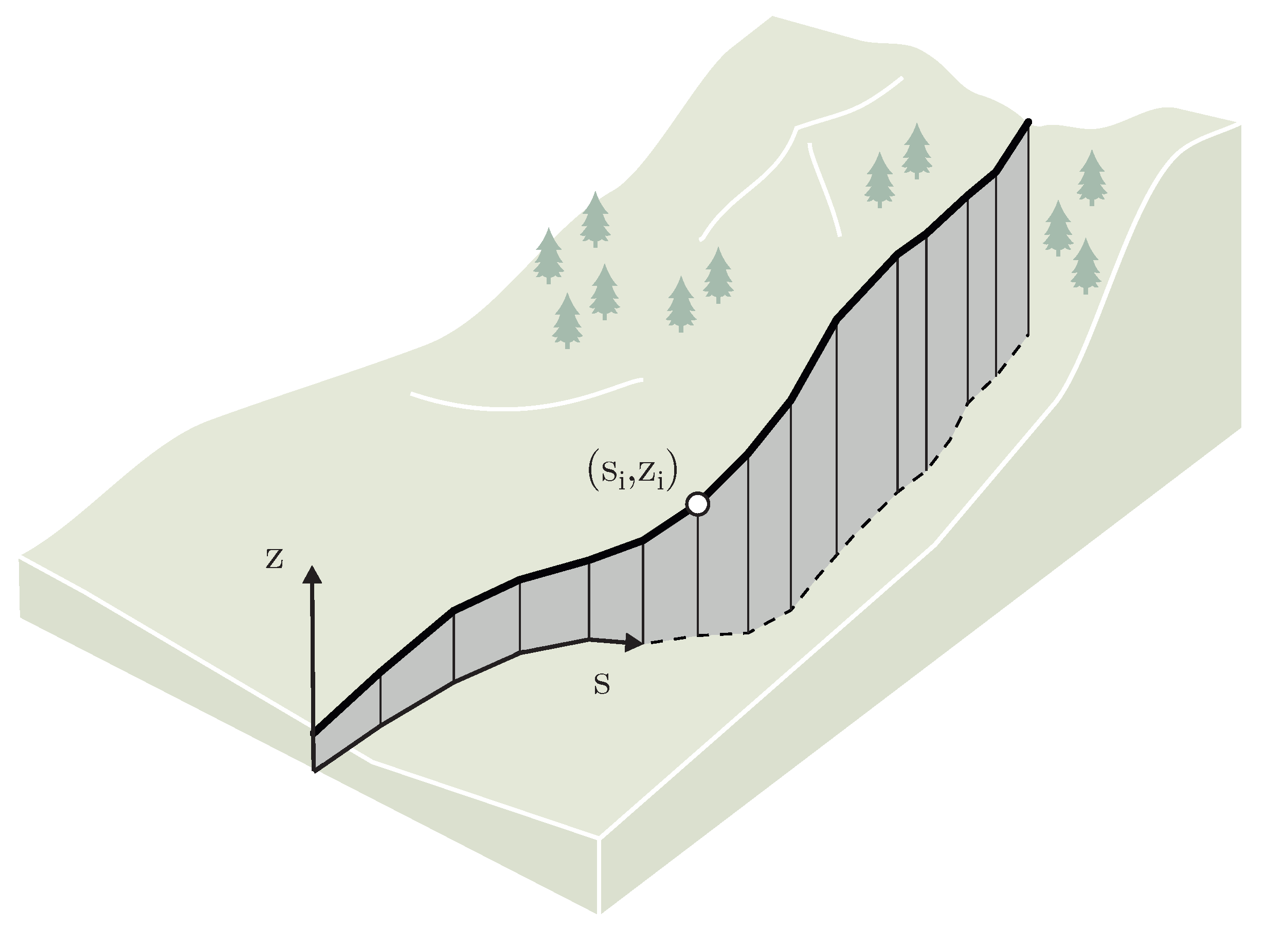
In order to model the different feasible layouts, the method in [29] is followed. According to this, the domain of the problem is defined as a -discretization of the height profile of the river, in the form of
where and represent, respectively, the horizontal and vertical location of the i-th point of the profile. Note that this profile is a 2D-development of a 3D-profile, as shown in Figure 3. It is relevant to note that the approximation of the real profile for its 2D-development requires several assumptions: first, the remote nature of the studied area is due to the mountainous geography, where the water sources are upper-course rivers, typically in V-shaped valleys, with low or negligible curvature (as will be seen in the real case studied in Section 5.4.6. In addition, the low population of these communities implies that the power requirements are especially low, requiring short penstocks. With these two considerations, it can be assumed that neglecting the 3D nature of the layout will not have noticeable implications on the formulation of the problem.
To model the solutions, the variable is defined as a set of N binary variables in the form of
which are defined in such a way that each combination of defines a layout of the MHPP. This is done as follows:
- Each represents the placement of an elbow in point .
- The minimal index i that makes represents the location of the powerhouse.
- The maximum index i that makes represents the location of the water intake (dam).
It is relevant to note the number of combinations for a typical problem. For instance, assuming a domain of 1 km, with a reasonable topographic resolution of 1 point each 5 m, results in points (higher in the case that the diameter is also considered). This represents a total of combinations, clearly an intractable problem for brute-force algorithms, which motivates the use of evolutionary computational approaches.
As an example of the explained formulation, a representative height profile with points is shown in Figure 4, together with the layout corresponding to a factible solution .
Once this model has been presented, the variables and L are needed to be expressed in terms of the solution . For this, it is easy to write the gross height, , as the height difference between the maximum and minimum points whose , this is
With respect to the length of the penstock, L, it can be determined as the sum of the lengths of each interval between two consecutive elbows, this is
3.2. Problem Formulation
The problem addressed in this work consists in finding the most suitable layout for the MHPP. This problem is addressed in both single-objective and multi-objective mode. In the first one, the cost of the plant C is minimized, while satisfying a set of constraints related to the generated power, P, and its practical feasibility of the plant. In the second one, the maximization of the power, P, is additionally considered for the same problem. The mentioned constraints are defined below.
3.2.1. Power Constraint
The main objective of the development of an MHPP is to guarantee that the power supply covers certain needs. In order to do that, once the community has been evaluated, a necessary power supply is established on the basis of covering a basic energy need. This generally includes illumination for each home and certain shared household appliances and entertainment devices such as a TV. The power needed to cover this supply, , is imposed in the form of a minimal generation constraint, which can be written as
Introducing (12) and (13) in this expression, the power constraint can be rewritten as
3.2.2. Flow Constraint
The flow rate available in the stream, , represents a limitation to the flow rate Q that can be extracted and used in the MHPP. For this reason, a constraint must be introduced to the problem so the solution does not imply an unfeasible value. In order to guarantee an adequate use of this resource, the constraint is introduced in terms of a fraction, , of the stream flow, , that is acceptable to be extracted. This can be written as
where represents the aforementioned portion (expressed per unit) of the water flow which can be extracted from its natural course. Introducing (12) and (13) in this expression, the flow constraint can be rewritten as
3.2.3. Feasibility Constraints
Finally, the feasibility of the layout is defined in this work in accordance with the layout and the terrain. To model this, two constraints are imposed:
- The pipe can be disposed at a certain height from the terrain (see points 4 and 5 in Figure 4), where the use of supports is assumed, only if this height remains under a maximum value, .
- The pipe can be disposed under a certain depth from the terrain (see points 8 and 9 in Figure 4), where excavations are assumed as part of the civil works, only if this depth remains under a maximum value, .
Parameters and are estimated in terms of the properties of the terrain and the available manpower. These constraints can be written as
4. Evolutionary Computational Approach
Evolutionary algorithms are meta-heuristic approaches that have been demonstrated to achieve significant results in complex optimization problems [46]. Among the evolutionary algorithms, Genetic Algorithms (GAs) have been widely used in many engineering optimization problems [47,48,49]. The main idea behind a GA is to encode potential solutions (individuals) in a chromosome-like structure in which each independent variable of the problem is codified as a gen of the chromosome. Thus, a list (population) of individuals evolves through several generations, creating new offspring that adapts better to the optimization landscape according to the survival of the fitness principle of the Darwinian theory. The higher the fitness of an individual, the better its adaptation to the search landscape. The adaptation of an individual is measured by means of its quality or fitness, that is, the evaluation of the solution as an input of the fitness function of the problem. The offspring is created by applying genetic operations, such as selection, crossover, and mutation. The selection consists of selecting the parents that will participate in the crossover and mutation operations. Selection is an elitist operation. Therefore, the higher the fitness of an individual, the higher the probability of being selected as a parent. The crossover operation consists of combining the genetic information of two individuals to create other two new individuals. Regarding the mutation, it modifies the genetic information of an individual to generate a new one. Both crossover and mutation are probabilistic operations. With a proper tuning of selection, crossover and mutation, GAs achieve good exploration and exploitation capabilities within the search landscape of the optimization problem. With respect to this work, an individual represents a possible design of the micro hydro power plant. Two configurations have been considered such as single-objective and multi-objective approaches. In the single-objective case, the fitness function is the cost of the plant. Therefore, it is a minimization problem. In the multi-objective case, the GA optimizes simultaneously two objectives such as cost (minimization) and power (maximization). In the multi-objective case, the optimization is achieved by applying a Pareto dominance-based technique, like the NSGA-II [50].
4.1. Single-Objective Optimization Problem
There are many possible implementations of single-objective GAs. In this work, a mupluslambda scheme has been used [51]. Algorithm 1 shows the implemented approach. It starts with a random initial population , which is evaluated. Then, the offspring is created by using crossover and mutation operations. and refer to the crossover and mutation probability, respectively. Next, the offspring is evaluated, and the new population is selected from the offspring generated and the previous population . This approach guarantees a good level of elitism since parents and offspring compete with each other to be selected for the next generation [51].
| Algorithm 1: GA mupluslambda. |
 |
Once the algorithm finishes, the resulting population contains the best solutions for the optimization problem. Normally, the stop criterion of the algorithm is a given number of generations.
4.1.1. Individual Representation
Each individual represents a possible design or layout of the MHPP. Therefore, the chromosome of each individual is a list containing ones or zeros (binary variables) according to (11). Each gen of the chromosome represents the placement of an elbow. In addition, the diameter of the pipes is also embedded in the chromosome by means of a binary codification, assuming that all pipes have the same diameter. The size S of the chromosome is 205 or 200 depending on whether the diameter of the pipes is considered or not (see Section 5 for more details). The first 200 bits correspond to the discrete data obtained from the profile of the river (see Figure 5a). When the diameter is embedded in the chromosome, the last five bits represent the diameter (see Figure 5a). Using five bits, 32 decimal numbers can be represented. According to (8), cannot be equal to 0, therefore the decimal numbers represented are within the interval , which determine the value of in centimeters. As mentioned in Section 3, the minimum index containing a one corresponds to the placement of the powerhouse (lowest position in the profile river) and maximum index containing a one corresponds to the location of the water intake (highest position in the profile river). The initial population of the GA is generated randomly. However, for the sake of generating feasible solutions in the initial step and avoiding discarding invalid ones, a tailored generator of initial individuals is proposed. The algorithm consists of selecting two random points and within the interval , being , and filling up with ones the positions within the interval (see Figure 5).
The resulting initial individual will not suffer from the feasibility constraints described in Section 3. This feature is important to guarantee an efficient exploration during the first generations of the GA.
4.1.2. Fitness Function
The fitness of each individual is given by the cost function (9). Therefore, the lower the cost, the better the solution is. However, invalid solutions should be discarded in order not to participate in future generations of the GA. Death penalty is used to penalized invalid individuals. As a result, the fitness of each individual will be calculated as
4.1.3. Genetic Operators
A tournament selection mechanism has been used since it provides suitable results [52]. In each tournament, a number of individuals are randomly selected, which compete with each other to be chosen as a parent; the best one is then selected as one of the parents to be used in crossover and mutation operations [52]. A tournament size of three has been demonstrated to be suitable for the majority of problems. Regarding the crossover operation, a two-point scheme has been used. It achieves good results for binary chromosomes. The two-point crossover consists of swapping the genetic information of two parents using two points as the indexes of the genetic exchange. As for the mutation algorithm, a tailored method is proposed. It consists of a modified flip-bit method. The probability of flipping a one to a zero is considerable higher than a zero to a one. The objective is to reduce the resulting cost of the layout. Please note that, with the proposed initial generator of individuals, the initial layouts have a high number of ones, therefore, a high cost. With the proposed mutation scheme, the cost of the individuals will be reduced progressively with the number of generations. Two values should be fixed and , which are the probability of converting a one to a zero and a zero to a one, respectively (see Section 5 for more details).
4.2. Multi-Objective Optimization Problem
In this case, the objective is to optimize simultaneously the cost (minimization) and the power generated (maximization) of the MHPP, according to (9) and (2), respectively. The multi-objective GA used is the NSGA-II [50], which is based on the Pareto dominance. It has been demonstrated to achieve good results in a wide range of engineering optimization problems. According to the Pareto dominance, a solution dominates another iff it is strictly superior in all considered objectives. Therefore, the aim of the NSGA-II is to find all non-dominated solutions, which form the so-called Pareto front. In the target optimization problem, the Pareto front will be a curve in the 2D dimensions resulting from the two objectives, cost and power.
Algorithm 2 shows the implemented multi-objective GA based Pareto dominance. The main difference with respect to the single-objective case are: (i) in the evaluation of the individuals for the two objectives should be calculated and (ii) the selection mechanism is based on the Pareto dominance. Notice that, at each iteration of the algorithm, the Pareto front is updated. Therefore, at the end of the algorithm, the Pareto front includes all non-dominated solutions found throughout the generations of the GA.
| Algorithm 2: GA based on NSGA-II. |
 |
The advantage of using a multi-objective approach is that the decision maker has a big picture of MHPP design. Therefore, other layouts can be considered if the conditions change in terms of budget, river profile, power required, etc.
4.2.1. Individual Representation
The individual representation is the same as that considered in the single-objective case.
4.2.2. Fitness Function
In this case, the fitness of each individual is a tuple of two components, one for each objective. Again, the death penalty is used to penalize invalid solutions. Such death penalty should be employed in each of the objectives. As a result, the fitness of each individual will be calculated as
4.2.3. Genetic Operators
The crossover and mutation schemes used are the same of the single-objective case.
5. Simulation Results
In this section, the application of the proposed evolutionary approach is discussed. For this, an example discretization of a river profile is first presented, the GA being applied to four different case-studies. Lastly, a set of real topographic data is used to verify the goodness of the proposed approach in a real case scenario.
5.1. Example Scenario Settings
The proposed example scenario consists of a discretization of points in the form of (10), represented in Figure 6 for a better understanding. For this river profile, the design of an MHPP is proposed to supply a hypothetical small community, whose basic power need is established in 8 kW. The flow of the river is 70 L/s, with an extraction allowance of 50%. In addition, an equivalent cost of 50 m is assumed for the installation of the elbows, and the characteristics of the terrain permit the installation of supports and excavations up to 1.5 m. The parameters associated to these constraints are summarized in Table 1.
5.2. Genetic Algorithm Settings
The design of the MHPP is addressed by means of a GA, by using the generation, crossover and mutation rules proposed in Section 4 (The code is available in [53]. The simulator has been developed using Python and DEAP [54].). Table 2 contains the main configuration parameters of the GA implementations.
5.3. Case-Studies Proposal
For this problem, four different scenarios are proposed (listed on Table 3), in ascending order of complexity:
- Case-study 1: Fixed diameter, without considering elbows. For this first case, a fixed pipe diameter is considered. The problem is formulated in the form of a cost-minimization problem in single-objective mode. The objective function is formulated as minimizing the length of the penstock, L.
- Case-study 2: Fixed diameter, considering an equivalent cost of the elbows. This second case consists in the problem proposed in case-study 1 with the additional consideration of an equivalent cost for the pipe elbows, . Thus, the objective function is formulated as minimizing the cost C.
- Case-study 3: Variable diameter, single-objective. In this third case, the problem in case 2 is extended by considering a range of available discrete values for the pipe diameter , this being considered as an additional optimization variable (see Figure 5a). The problem is then formulated in the form of a cost-minimization problem (single-objective mode), with the objective function formulated as minimizing the cost of the penstock, defined in terms of its length L, number of elbows and diameter .
- Case-study 4: Variable diameter, multi-objective. The last case is formulated on the same basis of case-study 2, but considering a multi-objective mode, where the cost of the plant is minimized and the generated power P is maximized.
5.4. Results
5.4.1. Case-Study 1: Fixed Diameter, without Considering Elbows
In this case, the diameter of the pipe is fixed, and thus the problem is formulated using
Note that this formulation matches the one proposed in [29], where the same problem is solved by using BBA-based methods, and thus the performance of this approach can be evaluated by comparing the results. The best solutions obtained using the GA for this case-study are listed in Table 4. In addition, in Figure 7, the best layout is represented over the river profile, where the layout corresponding to the reference solution [29] is also plotted.
Observing Table 4, it can be seen that the proposed approach leads to very similar solutions. Although GA solutions are strictly better than the proposed in the reference case [29], given the context of the real problem, the cost improvement (0.055%) is not very significant. It is relevant to note the effectiveness of the GA finding simple layouts with a low number of elbows (four instead of seven), even when this variable is not considered in the objective. This is due to the proposed mutation scheme, which tends to eliminate elbows from the layout.
5.4.2. Case-Study 2: Fixed Diameter, Considering an Equivalent Cost of the Elbows
This case study is modeled as the case-study 1, but considering the minimization of the cost defined in (9), using
This case-study is also solved in [29], and the solution can be directly compared to this reference. The best solutions obtained using the GA for this case-study are listed in Table 5. In addition, in Figure 8, the best layout is represented over the river profile, where the layout corresponding to the reference solution [29] is also plotted.
It can be seen that the GA provides a layout that provides the same gross height and water flow than the BBA algorithm, but requiring a slightly shorter penstock and four elbows instead of five, leading to an improvement of 11.78% with respect to the BBA.
5.4.3. Case-Study 3: Variable Diameter, Single-Objective
In this scenario, the diameter of the penstock, , is introduced as a new variable, where a noticeable improvement of the reference solution can be expected. The evolution of the Fitness value is represented in Figure 9, where it can be seen that the convergence is reached in the first 50 generations. This demonstrates the convergence of the GA for the proposed problem. Similar curves can be obtained for the other cases.
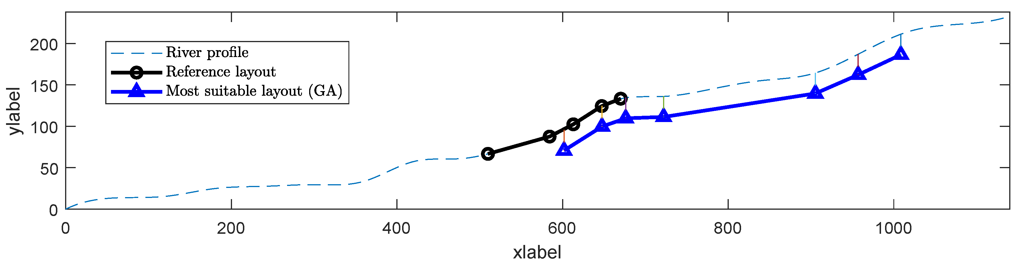
The solutions obtained for this case are summarized in Table 6. As expected, the possibility of varying the diameter of the penstock allows for finding new solutions with a noticeably lower cost. In Figure 10, the most suitable layout has been represented, together with the reference layout. Note that, although a higher gross height and a longer pipe are obtained, the smaller diameter provides a lower cost. The best solution obtained using the proposed GA provides an improvement of 70.67%, which is representative of the goodness of the proposed evolutionary approach, with respect to the BBA used in [29]. These require a linear formulation of the problem, and thus the diameter can not be assumed as a variable, due to the highly nonlinear effects in the MHPP performance.
5.4.4. Case-Study 4: Variable Diameter, Multi-Objective
This last case is proposed to discuss the adaptability of the multi-objective approach for this problem. A deeper study on the influente of the parameters is made by solving the same problem from case 2, considering a two-objective optimization algorithm. This mode provides a set of non-dominated solutions that correspond to optimal combinations of the objective values, forming the Pareto front [55]. This case combines the economic objective of minimizing the cost of the MHPP while maximizing the power generated. The results are shown in Figure 11, where the Pareto front is also represented.
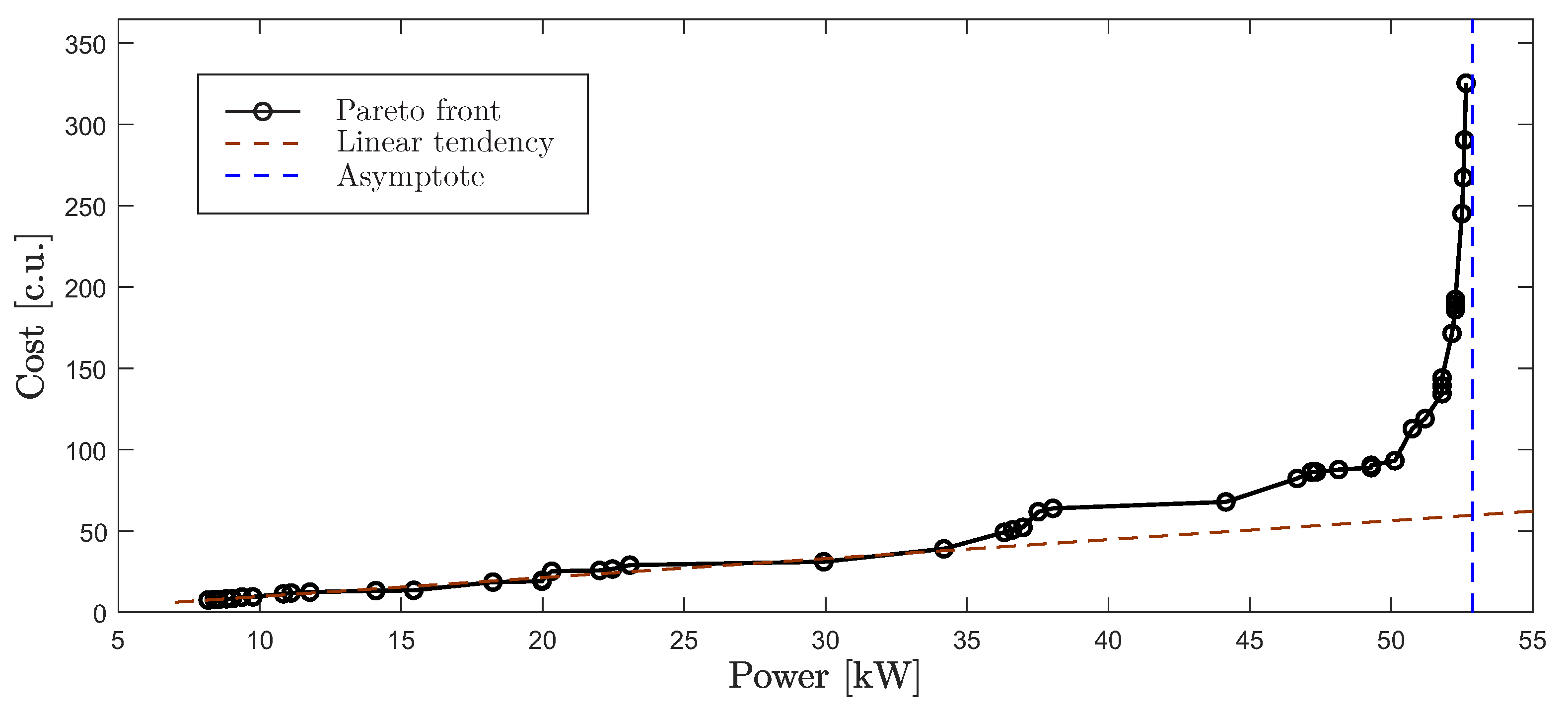
Observing the Pareto front, a few comments can be made. First, as expected, the competitive nature of the two objectives is made evident, as power cannot be increased without increasing the cost, and the opposite. Secondly, the Pareto front exhibits two distinct parts. It can be seen that the solutions with a low value of power and cost show an approximately linear tendency (represented with a red dashed line in Figure 12) in the Pareto front. This represents the capacity of increasing the domain of the MHPP on the river to reach a higher water head, and thus to obtain a higher power. The slope of this region can be estimated, resulting in 1.1671 c.u./kW, which represents that an increase of 10% in power would require increasing the cost in 12.63%.
However, this linear tendency abruptly changes for solutions with high values of power and cost, where the Pareto front shows an asymptotic behavior. Observing the solutions associated with these points, it can be understood that these solutions saturate the domain, and thus only small increases in power can be achieved by changing the combination of elbows and pipe lengths. To verify this, an upper level of the obtainable power can be estimated by considering a hypothetical solution (indicated by *) that exploits the maximum available height in the domain without friction loss; this can be done by substituting
in expression (8). This leads to
and it can be seen that the asymptote matches this value (represented with a blue dashed line in Figure 12).
5.4.5. Comparison with Other Algorithms
The proposed approach based on GA has been compared with other heuristic algorithms such as Simulated Annealing (SA) [56,57] and Random Search. The SA algorithm is trajectory-based algorithm, which uses probabilistic modifications (mutation) of an initial solution to guide it towards the global optimization points. Since the strength of the SA is its mutation capabilities, it is a good approach to measure the goodness of the proposed mutation scheme. Therefore, the SA implementation is based on two mutation schemes, as it can be observed in Figure 13, such as bit-flip and custom mutation. Regarding the random search, it has been used as a lower bound. According to the results included in Table 7, the GA-based approach clearly outperforms the other algorithms. It is important to remark that the SA algorithm achieves significantly better results when it implements the custom mutation. Therefore, it demonstrates that the proposed mutation scheme is suitable for the target optimization problem.
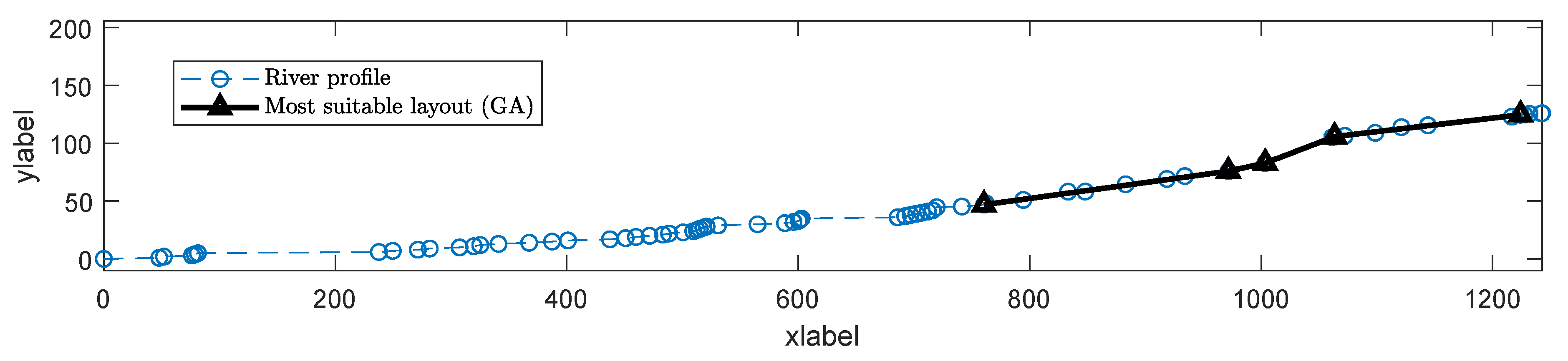
5.4.6. Application to a Real Scenario
In order to verify the goodness of the methodology to address a real-case problem, a set of data from a topographic survey has been used to optimize a MHPP. The selected scenario consists of a remote community located in the north area of Santa Bárbara, in Honduras. It has been excluded from the benefits of the national electrification grid, and, given its environmental characteristics, it has been considered by the local government to be supplied with an MHPP, providing the topographic survey of the terrain that is used in this section. The river layout is shown from an aerial view in Figure 14.
The parameters used for this problem (listed on Table 8) are the same from the previous examples, excepting the available flow, which is estimated in 50 L/s approximately. The solutions obtained for this case are summarized in Table 9. As the benefits of the proposed approach have already been verified in the previous examples, no additional algorithms have been used to address this problem. In Figure 15, the most suitable layout has been represented, together with the river layout.
Although these results can be directly compared to the results of the previous cases, two considerations must be taken into account. First, the average slope of the real scenario (101.4 m/km) is lower than the average slope of the example scenario (204.4 m/km), which can be directly interpreted as a lower intrinsic potential of the water resource. Secondly, as the real data is obtained from an empirical analysis, the data points are not uniformly distributed, as it happens to be in the proposed example. The existence of low-sampled areas in the domain hampers the possibility of finding optimal solutions that satisfy the constraints in the most efficient way.
5.5. Discussion of the Results
The present study has been carried out for developing a GA to address the problem of finding the most suitable layout for an MHPP that satisfies a set of constraints, which are formulated in terms of the power supply needs, water flow usage and feasibility, in order to be implemented in both an example and a real scenario. In sight of the results, the following conclusions can be formulated:
- An example scenario domain has been introduced first, in order to propose a total of four case-studies that have been addressed in order to validate the benefits of the GA to optimize an MHPP layout.
- When the objective function is assumed to be the minimization of the length of the penstock, the GA provides approximately the same solution than the BBA, with a slight improvement (about 0.055%) in the length, and reaching also a lower number of elbows, although it is not considered a design variable in the minimization function.
- The minimization of the equivalent cost leads to noticeabley better solutions, reaching an improvement of 11.78% in the cost, reducing both the length (about 0.05%) and the number of elbows (20%) of the penstock.
- The GA has been proven to be especially effective addressing the optimization problem when considering the penstock diameter as an optimization variable, leading to a cost reduction of 70.67%. Note that this problem can not be addressed by BBA-based due to its complexity, which implies nonlinearities in its formulation.
- In all the studied cases, the convergence is reached in the first 50 generations, with small improvements until the 100th generation.
- The problem has been addressed in a multi-objective mode, minimizing the cost and maximizing the generated power. The solutions have been used to determine the Pareto front, and, from this, the marginal rate of substitution, which allows for studying how variances in the cost can affect the performance of the plant.
- The problem has also been solved using Random Search and SA algorithms. Although the results of the random search algorithm and SA are poor and far from the optimal solutions obtained with the GA, the implementation of the proposed mutation scheme in the SA provides a noticeable improvement in its performance. Nevertheless, it reaches a reduction of 99.66% of the cost obtained with the SA. This noticeable difference is a consequence of the high number of elbows obtained by the SA algorithm (20 elbows obtained from SA facing five elbows obtained using GA), while the difference in length between the solutions is not that high (481.3 m using SA facing 175 m from GA).
- The GA has been successfully used to solve a real scenario problem, proving a good robustness when dealing with a low quality sampled domain.
6. Conclusions and Further Work
The proposed GA has demonstrated good performance addressing the problem of finding the most suitable layout for an MHPP, providing significant results in the case-studies evaluated. In general, the achieved results are better than the ones found in the literature, where a BBA is used. In addition, the GA approach is capable of addressing a more complex and realistic problem, where the penstock diameter is also considered as a design variable. This new problem, which can not be addressed by BBA due to its nonlinear nature, is successfully solved by the GA, and even better solutions are obtained, reaching a reduction of 70.67% of the cost, with respect to the solutions obtained by the BBA. Finally, it has been demonstrated that the GA is able to successfully address the multi-objective problem of maximizing the power in addition to minimizing the cost. This allows for obtaining the Pareto front, which has been used to determine the effects of varying the power and the cost of the plant. This is very useful to study the potential of the natural environment, which constitutes an excellent tool to assist the design of the MHPP and give a wider perspective of the problem.
In sight of the benefits of using GA to address the problem of optimizing the MHPP layout, and especially its capability to deal with more complex nonlinear problems, an extension of this work is proposed as a further work. The most immediate continuation of the presented work is the expansion of the problem into the 3D domain. This would guarantee that, unlike the usage of a 2D height profile development, the algorithm can be applied to rivers with a very winding route, as the layout would not be restricted to follow it. Although the high number of binary variables that would result from expanding to 3D the formulation used in this work would represent a drawback, a continuous approach of the surface and the MHPP layout can be used to deal with this issue.
Author Contributions
Conceptualization, Methodology Conceptualization: A.T.C., D.G.R. and P.M.G.; methodology and formal analysis: A.T.C. and D.G.R.; esults and data curation: D.G.R.; writing-Original Draft Preparation: A.T.C. and D.G.R.; review & Editing, D.G.R. and P.M.G.; All authors read and approved the final manuscript.
Funding
The research project on MHPP of which this work is part is supported by grant 2014/ACDE/006016 (AECID).
Conflicts of Interest
The authors declare no conflict of interest.
Abbreviations
The following abbreviations are used in this manuscript:
| BBA | Branch and Bound Algorithm |
| CCS | Carbon Capture and Storage |
| GA | Genetic Algorithm |
| GHG | Greenhouse Gas |
| HBMO | Honey Bee Mating Optimization |
| MHPP | Micro Hydro Power Plants |
| RES | Renewable Energy Sources |
| SA | Simulated Annealing |
References
- Nejat, P.; Jomehzadeh, F.; Taheri, M.M.; Gohari, M.; Majid, M.Z.A. A global review of energy consumption, CO2 emissions and policy in the residential sector (with an overview of the top ten CO2 emitting countries). Renew. Sustain. Energy Rev. 2015, 43, 843–862. [Google Scholar] [CrossRef]
- The World Bank. Access to Electricity. World Development Indicators. 2016. Available online: http://data.worldbank.org/indicator/EG.ELC.ACCS.UR.ZS (accessed on 2 December 2018).
- Pereira, M.G.; Sena, J.A.; Freitas, M.A.V.; Da Silva, N.F. Evaluation of the impact of access to electricity: A comparative analysis of South Africa, China, India and Brazil. Renew. Sustain. Energy Rev. 2011, 15, 1427–1441. [Google Scholar] [CrossRef]
- OECD. Linking Renewable Energy to Rural Development, OECD Green Growth Studies; OECD Publishing: Paris, France, 2016. [Google Scholar]
- Krewitt, W.; Simon, S.; Graus, W.; Teskec, S.; Zervos, A.; Schafer, O. The 2 degrees C scenario-A sustainable world energy perspective (vol 35, pg 4969, 2007). Energy Policy 2008, 36, 494. [Google Scholar] [CrossRef]
- Luderer, G.; Krey, V.; Calvin, K.; Merrick, J.; Mima, S.; Pietzcker, R.; Van Vliet, J.; Wada, K. The role of renewable energy in climate stabilization: Results from the EMF27 scenarios. Clim. Chang. 2014, 123, 427–441. [Google Scholar] [CrossRef]
- REN21 Renewables Global Status Report: 2009. Available online: http://www.unep.fr/shared/docs/publications/RE_GSR_2009_Update.pdf (accessed on 21 November 2018).
- Kanase-Patil, A.; Saini, R.; Sharma, M. Integrated renewable energy systems for off grid rural electrification of remote area. Renew. Energy 2010, 35, 1342–1349. [Google Scholar] [CrossRef]
- Bugaje, I. Renewable energy for sustainable development in Africa: A review. Renew. Sustain. Energy Rev. 2006, 10, 603–612. [Google Scholar] [CrossRef]
- Sahoo, S.K. Renew. Sustain. Energy Rev. solar photovoltaic energy progress in India: A review. Renew. Sustain. Energy Rev. 2016, 59, 927–939. [Google Scholar] [CrossRef]
- Saheb-Koussa, D.; Haddadi, M.; Belhamel, M. Economic and technical study of a hybrid system (wind–photovoltaic–diesel) for rural electrification in Algeria. Appl. Energy 2009, 86, 1024–1030. [Google Scholar] [CrossRef]
- Mohammed, Y.; Mokhtar, A.; Bashir, N.; Saidur, R. An overview of agricultural biomass for decentralized rural energy in Ghana. Renew. Sustain. Energy Rev. 2013, 20, 15–25. [Google Scholar] [CrossRef]
- Sachdev, H.S.; Akella, A.K.; Kumar, N. Analysis and evaluation of small hydropower plants: A bibliographical survey. Renew. Sustain. Energy Rev. 2015, 51, 1013–1022. [Google Scholar] [CrossRef]
- Gaglia, A.; Kaldellis, J.; Kavadias, K.; Konstantinidis, P.; Sigalas, J.; Vlachou, D. Integrated studies on renewable energy sources. The soft energy application laboratory, mechanical engineering department, TEI of Piraeus. In World Renewable Energy Congress VI; Elsevier: Amsterdam, The Netherlands, 2000; pp. 1588–1591. [Google Scholar]
- Al Irsyad, M.I.; Halog, A.; Nepal, R. Renewable energy projections for climate change mitigation: An analysis of uncertainty and errors. Renew. Energy 2019, 130, 536–546. [Google Scholar] [CrossRef]
- Jawahar, C.; Michael, P.A. A review on turbines for micro hydro power plant. Renew. Sustain. Energy Rev. 2017, 72, 882–887. [Google Scholar] [CrossRef]
- World Bank. Technical and Economic Assessment of Off Grid, Mini-Grid and Grid Electrification Technologies; Energy Sector Management Assistance Program (ESMAP) Technical Paper Series, ESM 212/07; World Bank: Washington, DC, USA, 2007. [Google Scholar]
- Khurana, S.; Kumar, A. Small hydro power—A review. Int. J. Therm. Technol. 2011, 1, 107–110. [Google Scholar]
- Mandelli, S.; Barbieri, J.; Mereu, R.; Colombo, E. Off-grid systems for rural electrification in developing countries: Definitions, classification and a comprehensive literature review. Renew. Sustain. Energy Rev. 2016, 58, 1621–1646. [Google Scholar] [CrossRef]
- Carravetta, A.; Derakhshan Houreh, S.; Ramos, H.M. Pumps as Turbines; Springer Tracts in Mechanical Engineering; Springer: Berlin/Heidelberg, Germany, 2018. [Google Scholar]
- Sangal, S.; Garg, A.; Kumar, D. Review of optimal selection of turbines for hydroelectric projects. Int. J. Emerg. Technol. Adv. Eng. 2013, 3, 424–430. [Google Scholar]
- Herschy, R.W. Chapter 10. Weirs and flumes. In Streamflow Measurement; CRC Press: Boca Raton, FL, USA, 2014; Volume 3. [Google Scholar]
- Thake, J. Micro-Hydro Pelton Turbine Manual: Design, Manufacture and Installation for Small-Scale Hydropower; Practical ACtion Publishing: Warwickshire, UK, 2000; pp. 136–142. [Google Scholar]
- Mishra, S.; Singal, S.; Khatod, D. Optimal installation of small hydropower plant—A review. Renew. Sustain. Energy Rev. 2011, 15, 3862–3869. [Google Scholar] [CrossRef]
- Elbatran, A.; Yaakob, O.; Ahmed, Y.M.; Shabara, H. Operation, performance and economic analysis of low head micro-hydropower turbines for rural and remote areas: A review. Renew. Sustain. Energy Rev. 2015, 43, 40–50. [Google Scholar] [CrossRef]
- Bozorg Haddad, O.; Moradi-Jalal, M.; Marino, M.A. Design–operation optimisation of run-of-river power plants. In Proceedings of the Institution of Civil Engineers-Water Management; Thomas Telford Ltd.: London, UK, 2011; Volume 164, pp. 463–475. [Google Scholar]
- Anagnostopoulos, J.S.; Papantonis, D.E. Optimal sizing of a run-of-river small hydropower plant. Energy Convers. Manag. 2007, 48, 2663–2670. [Google Scholar] [CrossRef]
- Alexander, K.V.; Giddens, E.P. Optimum penstocks for low head microhydro schemes. Renew. Energy 2008, 33, 507–519. [Google Scholar] [CrossRef]
- Tapia, A.; Millán, P.; Gómez-Estern, F. Integer programming to optimize Micro-Hydro Power Plants for generic river profiles. Renew. Energy 2018, 126, 905–914. [Google Scholar] [CrossRef]
- Gingold, P. The optimum size of small run-of-river plants. Int. Water Power Dam Constr. 1981, 33, 2663–2670. [Google Scholar]
- Ehteram, M.; Karami, H.; Mousavi, S.F.; Farzin, S.; Kisi, O. Evaluation of contemporary evolutionary algorithms for optimization in reservoir operation and water supply. J. Water Supply Res. Technol.-Aqua 2018, 67, 54–67. [Google Scholar] [CrossRef]
- Aslan, Y.; Arslan, O.; Yasar, C. A sensitivity analysis for the design of small-scale hydropower plant: Kayabogazi case study. Renew. Energy 2008, 33, 791–801. [Google Scholar] [CrossRef]
- Williamson, S.; Stark, B.; Booker, J. Low head pico hydro turbine selection using a multi-criteria analysis. Renew. Energy 2014, 61, 43–50. [Google Scholar] [CrossRef]
- Singal, S.; Saini, R.; Raghuvanshi, C. Analysis for cost estimation of low head run-of-river small hydropower schemes. Energy Sustain. Dev. 2010, 14, 117–126. [Google Scholar] [CrossRef]
- Banos, R.; Manzano-Agugliaro, F.; Montoya, F.; Gil, C.; Alcayde, A.; Gómez, J. Optimization methods applied to renewable and sustainable energy: A review. Renew. Sustain. Energy Rev. 2011, 15, 1753–1766. [Google Scholar] [CrossRef]
- Iqbal, M.; Azam, M.; Naeem, M.; Khwaja, A.; Anpalagan, A. Optimization classification, algorithms and tools for renewable energy: A review. Renew. Sustain. Energy Rev. 2014, 39, 640–654. [Google Scholar] [CrossRef]
- Bozorg-Haddad, O.; Loáiciga, H.A. Honey-Bee Mating Optimization; John Wiley and Sons, Ltd.: Hoboken, NJ, USA, 2017; Chapter 12; pp. 145–161. [Google Scholar] [CrossRef]
- Basso, S.; Botter, G. Streamflow variability and optimal capacity of run-of-river hydropower plants. Water Resour. Res. 2012, 48. [Google Scholar] [CrossRef] [Green Version]
- Yoo, J.H. Maximization of hydropower generation through the application of a linear programming model. J. Hydrol. 2009, 376, 182–187. [Google Scholar] [CrossRef]
- Bragalli, C.; D’Ambrosio, C.; Lee, J.; Lodi, A.; Toth, P. On the optimal design of water distribution networks: A practical MINLP approach. Optim. Eng. 2012, 13, 219–246. [Google Scholar] [CrossRef]
- Fecarotta, O.; McNabola, A. Optimal location of pump as turbines (PATs) in water distribution networks to recover energy and reduce leakage. Water Resour. Res. 2017, 31, 5043–5059. [Google Scholar] [CrossRef]
- Fecarotta, O.; Carravetta, A.; Morani, M.; Padulano, R. Optimal Pump Scheduling for Urban Drainage under Variable Flow Conditions. Resources 2018, 7, 73. [Google Scholar] [CrossRef]
- Alexander, K.V.; Giddens, E.P. Microhydro: Cost-effective, modular systems for low heads. Renew. Energy 2008, 33, 1379–1391. [Google Scholar] [CrossRef]
- Leon, A.S.; Zhu, L. A dimensional analysis for determining optimal discharge and penstock diameter in impulse and reaction water turbines. Renew. Energy 2014, 71, 609–615. [Google Scholar] [CrossRef]
- Green, D.W. Perry’s Chemical Engineers’ Handbook, 8th ed.; McGraw-Hill: New York, NY, USA, 2008. [Google Scholar]
- Holland, J.H. Genetic Algorithms and Adaptation; Springer: Boston, MA, USA, 1984; pp. 317–333. [Google Scholar] [CrossRef]
- Reina, D.; Camp, T.; Munjal, A.; Toral, S. Evolutionary deployment and local search-based movements of 0th responders in disaster scenarios. Future Gener. Comput. Syst. 2018, 88, 61–78. [Google Scholar] [CrossRef]
- Arzamendia, M.; Gregor, D.; Reina, D.G.; Toral, S.L. An evolutionary approach to constrained path planning of an autonomous surface vehicle for maximizing the covered area of Ypacarai Lake. Soft Comput. 2017, 23, 1723–1734. [Google Scholar] [CrossRef]
- Gutiérrez-Reina, D.; Sharma, V.; You, I.; Toral, S. Dissimilarity Metric Based on Local Neighboring Information and Genetic Programming for Data Dissemination in Vehicular Ad Hoc Networks (VANETs). Sensors 2018, 18, 2320. [Google Scholar] [CrossRef] [PubMed]
- Deb, K.; Pratap, A.; Agarwal, S.; Meyarivan, T. A fast and elitist multiobjective genetic algorithm: NSGA-II. IEEE Trans. Evol. Comput. 2002, 6, 182–197. [Google Scholar] [CrossRef] [Green Version]
- Ter-Sarkisov, A.; Marsland, S. Convergence Properties of Two ({∖mu}+{∖lambda}) Evolutionary Algorithms On OneMax and Royal Roads Test Functions. arXiv, 2011; arXiv:1108.4080. [Google Scholar]
- Luke, S. Essentials of Metaheuristics; Lulu Raleigh: San Francisco, CA, USA, 2009; Volume 113. [Google Scholar]
- Gutierrez, D. Evolutionary MHPP. 2018. Available online: https://github.com/Dany503/Evolutionary-MHPP (accessed on 11 December 2018).
- Fortin, F.A.; Rainville, F.M.D.; Gardner, M.A.; Parizeau, M.; Gagné, C. DEAP: Evolutionary algorithms made easy. J. Mach. Learn. Res. 2012, 13, 2171–2175. [Google Scholar]
- G Reina, D.; Ciobanu, R.; Toral, S.; Dobre, C. A Multi-objective Optimization of Data Dissemination in Delay Tolerant Networks. Expert Syst. Appl. 2016, 57, 178–191. [Google Scholar] [CrossRef]
- Kirkpatrick, S.; Gelatt, C.D.; Vecchi, M.P. Optimization by Simulated Annealing. Science 1983, 220, 671–680. [Google Scholar] [CrossRef] [PubMed] [Green Version]
- Leitold, D.; Vathy-Fogarassy, A.; Abonyi, J. Network Distance-Based Simulated Annealing and Fuzzy Clustering for Sensor Placement Ensuring Observability and Minimal Relative Degree. Sensors 2018, 18, 3096. [Google Scholar] [CrossRef] [PubMed]
Figure 1.
Scheme of a typical MHPP.

Figure 2.
Working scheme of a Pelton turbine (left) and Turgo turbine (right).

Figure 3.
2D simplification of the river profile.

Figure 4.
MHPP layout associated with the solution , for an illustrative river profile discretization with points. Please note that the formation of gaps between the terrain and the penstock in certain points.
Figure 4.
MHPP layout associated with the solution , for an illustrative river profile discretization with points. Please note that the formation of gaps between the terrain and the penstock in certain points.

Figure 5.
Individual representation considering the diameter of the penstock (a) and individual generation scheme (b).
Figure 5.
Individual representation considering the diameter of the penstock (a) and individual generation scheme (b).

Figure 6.
Example river profile (blue line). The topographic data points have been marked (black dots) to emphasize its uniform distribution.
Figure 6.
Example river profile (blue line). The topographic data points have been marked (black dots) to emphasize its uniform distribution.

Figure 7.
Most suitable layout for case-study 1 (blue) and reference solution (black).

Figure 8.
Most suitable layout for case-study 2 (blue) and reference solution (black).

Figure 9.
Evolution of fitness for case-study 3.

Figure 10.
Most suitable layout for case-study 3 (blue) and reference solution (black).

Figure 11.
Solutions obtained (blue) and Pareto front (black).

Figure 12.
Pareto front (black), with the two observable tendencies (linear behavior in red, asymptote in blue) shown.
Figure 12.
Pareto front (black), with the two observable tendencies (linear behavior in red, asymptote in blue) shown.

Figure 13.
Most suitable layout obtained using Random Search and Simulated Annealing, compared to the obtained with the GA in study-case 3.
Figure 13.
Most suitable layout obtained using Random Search and Simulated Annealing, compared to the obtained with the GA in study-case 3.

Figure 14.
Aerial view of the studied river profile (black) and a small tributary (white).

Figure 15.
Most suitable layout (black) for the real scenario (blue). The topographic data has been marked (circles) to show its irregular distribution.
Figure 15.
Most suitable layout (black) for the real scenario (blue). The topographic data has been marked (circles) to show its irregular distribution.


Table 1.
Parameters of the example problem.
| Parameter | Value | Unit |
|---|---|---|
| 8 | kW | |
| 70 | L/s | |
| 0.5 | - | |
| 50 | m | |
| 1.5 | m | |
| 1.5 | m |
Table 2.
Parameters of the GA.
| Parameter | Value |
|---|---|
| 2000 | |
| 2000 | |
| Individuals (multi-objective) | 2000 |
| Generations | 100 |
| Selection | Tournament size = 3 (single-objective) NSGA-II (multi-objective) |
| Crossover | Two-point scheme |
| Mutation | Modified bitflip , , |
| Number of trials | 30 |
Table 3.
Description of the case-studies.
| Case | Objective Function | Pipe Diameter |
|---|---|---|
| Case-study 1 | min L (13) | Fixed |
| Case-study 2 | min C (9) | Fixed |
| Case-study 3 | min C (9) | Variable |
| Case-study 4 | min C (9), max P (8) | Variable |
Table 4.
Best solutions for case-study 1.
| Genetic Algorithm | BBA [29] | |||
|---|---|---|---|---|
| 0.80 | 0.70 | 0.60 | ||
| 0.20 | 0.30 | 0.40 | ||
| Gross height (m) | 66.648 | 66.648 | 66.648 | 66.648 |
| Flow rate (L/s) | 13.718 | 13.718 | 13.718 | 13.718 |
| Power (kW) | 8.064 | 8.064 | 8.064 | 8.064 |
| Number of elbows | 4 | 4 | 4 | 7 |
| Length (m) | 174.903 | 174.903 | 174.903 | 174.999 |
Table 5.
Best solutions for case-study 2.
| Genetic Algorithm | BBA [29] | |||
|---|---|---|---|---|
| 0.80 | 0.70 | 0.60 | ||
| 0.20 | 0.30 | 0.40 | ||
| Gross height (m) | 66.648 | 66.648 | 66.648 | 66.648 |
| Flow rate (L/s) | 13.718 | 13.718 | 13.718 | 13.718 |
| Power (kW) | 8.039 | 8.039 | 8.039 | 8.039 |
| Length (m) | 174.9240 | 174.9240 | 174.9240 | 175.005 |
| Number of elbows | 4 | 4 | 4 | 5 |
| Cost (m) | 14.997 | 14.997 | 14.997 | 17.000 |
Table 6.
Best solutions for case-study 3.
| Genetic Algorithm | BBA [29] | |||
|---|---|---|---|---|
| 0.80 | 0.70 | 0.60 | ||
| 0.20 | 0.30 | 0.40 | ||
| Gross height (m) | 78.919 | 115.642 | 115.642 | 66.648 |
| Flow rate (L/s) | 13.7863 | 13.7127 | 13.7128 | 13.718 |
| Power (kW) | 8.160 | 8.030 | 8.030 | 8.039 |
| Length (m) | 310.754 | 429.114 | 429.103 | 175.005 |
| Number of elbows | 5 | 7 | 7 | 5 |
| Pipe diameter (cm) | 10 | 8 | 8 | 20 |
| Cost (c.u.) | 5.608 | 4.986 | 4.986 | 17.000 |
Table 7.
Results for Random Search and Simulated Annealing.
| Random Search | Simulated Annealing | Reference [29] | ||
|---|---|---|---|---|
| Bit Flip | Custom Mutation | |||
| Gross height (m) | 226.192 | 216.005 | 123.513 | 66.648 |
| Flow rate (L/s) | 14.601 | 14.491 | 13.819 | 13.718 |
| Power (kW) | 9.695 | 9.477 | 8.217 | 8.039 |
| Length (m) | 1159.8 | 1106.8 | 481.3 | 175.005 |
| Number of elbows | 99 | 63 | 20 | 5 |
| Pipe diameter (cm) | 8 | 8 | 8 | 20 |
| Cost (c.u.) | 6109.8 | 4256.8 | 1481.3 | 17.000 |
Table 8.
Parameters of the real scenario problem.
| Parameter | Value | Unit |
|---|---|---|
| 8 | kW | |
| 50 | L/s | |
| 0.5 | - | |
| 50 | m | |
| 1.5 | m | |
| 1.5 | m |
Table 9.
Best solutions for the real scenario.
| Genetic Algorithm | |||
|---|---|---|---|
| 0.80 | 0.70 | 0.60 | |
| 0.20 | 0.30 | 0.40 | |
| Gross height (m) | 86.664 | 77.756 | 77.756 |
| Flow rate (L/s) | 15.445 | 14.654 | 14.654 |
| Power (kW) | 11.473 | 9.800 | 9.800 |
| Length (m) | 536.247 | 471.740 | 471.740 |
| Number of elbows | 8 | 5 | 5 |
| Pipe diameter (cm) | 16 | 16 | 16 |
| Cost (c.u.) | 23.968 | 18.4765 | 18.4765 |
© 2019 by the authors. Licensee MDPI, Basel, Switzerland. This article is an open access article distributed under the terms and conditions of the Creative Commons Attribution (CC BY) license (http://creativecommons.org/licenses/by/4.0/).
Share and Cite
MDPI and ACS Style
Tapia Córdoba, A.; Gutiérrez Reina, D.; Millán Gata, P. An Evolutionary Computational Approach for Designing Micro Hydro Power Plants. Energies 2019, 12, 878. https://doi.org/10.3390/en12050878
AMA Style
Tapia Córdoba A, Gutiérrez Reina D, Millán Gata P. An Evolutionary Computational Approach for Designing Micro Hydro Power Plants. Energies. 2019; 12(5):878. https://doi.org/10.3390/en12050878
Chicago/Turabian StyleTapia Córdoba, Alejandro, Daniel Gutiérrez Reina, and Pablo Millán Gata. 2019. "An Evolutionary Computational Approach for Designing Micro Hydro Power Plants" Energies 12, no. 5: 878. https://doi.org/10.3390/en12050878
Note that from the first issue of 2016, this journal uses article numbers instead of page numbers. See further details here.