Transient Stability Prediction for Real-Time Operation by Monitoring the Relative Angle with Predefined Thresholds


1
Applied Technologies Research Group GITA, Universidad Nacional de Colombia, Sede Medellín 050041, Colombia
2
Department of Electrical Energy and Automation, Universidad Nacional de Colombia, Sede Medellín 050041, Colombia
3
National Control Center, XM, Operator of the Colombian Power System, Medellín 050022, Colombia
*
Author to whom correspondence should be addressed.
Energies 2019, 12(5), 838; https://doi.org/10.3390/en12050838
Submission received: 16 January 2019
/
Revised: 13 February 2019
/
Accepted: 25 February 2019
/
Published: 4 March 2019
(This article belongs to the Section F: Electrical Engineering)
Abstract
:Under real-time operation, early detection of oscillations that lead to instability is of noteworthy importance for power system operators. This paper demonstrates how the relative angle (RA) obtained with online data from phasor measurement units (PMUs) and predefined thresholds of the relative angle (PTRA) obtained with offline simulations are valuable for the monitoring and prediction of transient stability. Primary features of the method consist of first calculating the maximum and minimum relative angles by offline simulations of different contingencies. Next, the voltage angles at buses that represent areas of the power system are measured to calculate the center of inertia (COI). Finally, the RA of the generators at each area is determined during the online operation to monitor stability behaviors and identify those that lead to a loss of synchronism. The method was validated in the New England 39-bus and the IEEE 118-bus power systems by performing contingencies, finding critical stability angles, monitoring areas and controlling the predicted unstable events with control actions, such as generation and load tripping, with enough time to return to stability.
1. Introduction
Nowadays, power systems are operated closer to their safety limits and some disturbances can produce instabilities that lead to service interruption or blackouts [1]. Therefore, real-time monitoring is important for electricity companies and new applications for power system security are still needed. Nevertheless, in recent years, phasor measurement unit (PMU) installations have increased considerably, allowing the availability of real-time data that show the system’s dynamic operating behavior [2]. This opens the possibility to develop an efficient monitoring application for more robust and secure power systems.
Usually, angular stability studies are carried out for the first swing, after the clearance of disturbances [3]. However, the first swing could show a stable operation and the subsequent oscillations lead to a loss of synchronism due to small disturbances [4]. Those angular behaviors that lead to instability are not easily detected because some state estimators could be considering unsynchronized data from the supervisory control and data acquisition (SCADA), where the deviation is mainly due to the asymmetrical time between measurements [5]. These anomalies can be removed with the use of synchronized measurements [6], that have time stamps referenced by the global positioning system (GPS) to eliminate deviations from the geographic distribution and the separation of power systems. Hence, the use of PMUs with computational and communication advances which facilitate the online monitoring of the power system’s dynamic behavior [7].
This paper focuses on using PMU data to monitor the rotor angle during transient stability events. Many investigations have been conducted related to this topic. For example, in Reference [8], a fast transient stability prediction using pattern recognition was proposed where the method saved an extensive database of rotor angle trajectories simulated for several faults in the power system and then compared these with the most similar trajectory detected by calculating the Euclidean distance; however, the method is sensitive to the selection of a trajectory mode and the prediction can be completely different to the real oscillation of the generator angle. In Reference [5], PMUs were used to predict the loss of synchronism with the energy function and the Lyapunov direct method and instability was detected faster compared with the traditional impedance relay; however, this was not applied for multi-machine systems. In Reference [9], a hybrid method was proposed by updating tables with online data of vulnerable areas and using off-line dynamic simulations, to identify the generators to be disconnected, once the loss of synchronism is predicted by online measurements; however, data must be updated every 20 minutes due to possible topological changes in the network or to re-dispatch, which is a problem when considering the continuous changes in the network.
In Reference [10], the authors analyzed the behavior of the power system through the separation of two groups: critical and non-critical machines; thus, the critical machines group helped assess the stability by means of converting the system to one equivalent machine and one infinite bus, and using the equal area criterion. Even more, a single machine equivalent model was proposed for the transient stability prediction in Reference [1], which considers data from PMUs after a disturbance adds the critical and non-critical machines in two equivalent groups. Subsequent transient stability is inferred from the single machine equivalent model through the equal area criterion, providing essential information, stability margins, and critical machines. In Reference [11], the transient instability was predicted by an improved Prony algorithm. The results show that this is simpler than detection by the impedance relay; however, the method is not stable and accurate when the exponents of the algorithm are not selected properly.
Some authors have mainly focused on the first swing and not on subsequent oscillations that can lead the power system to transient instability. Some studies have presented an evaluation of stability and the prediction of critical events once the power system has not had enough time to perform control actions. Other studies present the prediction of instability with the last oscillation and with the estimation of rotor angle, which is complex to obtain in real-time operations. Others use equivalents that are not easy to obtain with different network topologies or use a single machine. Finally, other authors use databases of events that can be outdated after several minutes due to continuous changes in the network.
The method presented in this paper considers the following features not included in previous works. Predefined thresholds of the relative angle (PTRA) are obtained to represent the maximum and minimum limits that the relative angle (RA) can reach after a contingency. Online center of inertia (COI) and RA are calculated continually to evaluate the behavior of the power system. An index is proposed to evaluate how close the RA is from the limits. Data obtained from PMUs at generation buses represent areas of the power system. The presented algorithm is useful for more secure and reliable operation as it works as a criterion against loss of synchronism. Furthermore, this simple method monitors the continuous transient stability of generators and areas, and predicts instability when the RAs reach the PTRA, with enough time to perform control actions.
The rest of the document has been divided into three sections. Section 2 presents the material and methods, including the problem formulation and algorithm development. Section 3 presents the simulations, the results, the analysis, and discussion. Finally, Section 4 presents conclusions and recommendations for future work.
2. Materials and Methods
In this section, the angle stability theory, rotor angles trajectories, the relative angle thresholds are formulated. The offline and online algorithms with the steps used to predict the transient instability are also included.
2.1. Angle Stability Analysis
Angle stability refers to the ability of generators connected to the power system to remain synchronous after being subjected to a disturbance [12,13], and depends on the ability to maintain or restore balance among the torques that affect the machine. However, the mechanical power of the generator does not change instantly and involves large excursions in the rotor angle of generators, which is influenced by the non-linear relationship between the real power and the angle [14].
Therefore, the mechanical power must be equal to the electrical power before the disturbance as shown in Equation (1) neglecting friction and damping losses. In this case, power losses are neglected and the term , which is the accelerating power (left part of the equation) can be written as , where the term is the mechanical power and is the electrical power. We introduce as the inertia constant and as the rotor angle of the system to obtain:
When a fault occurs, the electrical power changes abruptly and the mechanical power is maintained, producing acceleration or deceleration in the rotor angles of generators. Thus, the expression shown in Equation (1) is useful to calculate the absolute angles and the angular tendency by extrapolating the variables calculated for a system with multiple generators [15].
In Equation (1), the electrical power must be equal to the power transfer to the terminal bus of each machine as defined in Equation (2), where is the power that flows from to the terminal bus of the system, is the voltage in bus , is the voltage in bus , is the admittance that connects the element between and , is the angle of the element connected between and , is the voltage angle in , and is the voltage angle in . In this case, the term corresponds to an internal point in the machine and to the bus that connects the terminal of the machine:
Voltage in the terminal of the machine () is calculated with Equation (3), where is the internal voltage of the machine, is the internal resistance of the machine, is the current flowing from the machine to the terminal bus of generator j, and is the transient reactance of the generator :
A power system with n buses and m generators, represented by dynamic models, is considered in this research. Then, the behavior of the rotor angle of a synchronous generator is defined as shown in Equation (4), where i = 1, 2, 3, … m represents the number of generators, and is the angular frequency of the system:
The dynamic behavior of the power system during transient stability are determined with Equations (1) and (4) [16]. The solutions of these equations represent the dynamic behavior of the power system in the time domain and allow determining the response of all the studied variables (i.e., , ). However, finding such solutions during online operation has proven to be quite inefficient because these techniques are computationally demanding and require extensive memory to predict and assess the dynamic behavior of the power system for real-time operation. In addition, to find a good solution, it is necessary to know in detail the topology of the electrical network.
2.2. Rotor Angle Trajectories
When a fault occurs, the electric power supplied to the system changes and the mechanical power remains constant, instantly producing differences between the values of the electromagnetic torque and mechanical torque and resulting in a rotor speed increase or decrease with highly non-linear variation [3], This results in a change in the RA, which can be calculated and used to determine a reference similar to the use of the COI, and subsequently, the stability index to predict the loss of synchronism during transient events.
Currently, from the perspective of online stability prediction, it is complex to analyze the dynamic behavior of the whole power system. However, it is possible to achieve a characteristic trajectory of the generators by simulations and short-term real-time data and priority information of the bus phase angle supplied by PMUs to identify when the rotor angle trajectory moves away and causes a loss of synchronism.
The phase angle and the relative phase difference can change significantly in the power system, which is determined by the power transfer and the available transmission lines of the power system. The predicted loss of synchronism between generators when the system is subjected to a disturbance can be observed through the rotor angle variations [17]. Rotor angle is calculated with respect to a reference machine; however, this can be calculated with respect to the RA of the power system, which is a common transformation used for transient stability analysis.
For a system that contains multiple machines, the transient stability can be predicted using the RA. The COI is an index associated with each area based on equivalent inertia and rotor angles represented by a group of generators in area [2]. The COI is useful because it describes the transient behavior of the angle with respect to the RA of the system and not only a reference machine [4,18]. The COI also has the advantage of being more symmetrical in terms of identifying the angle trajectories because a generation plant or area may eventually lose synchronism with respect to the power system and this could be not detected by the protection relays.
Assuming that all generators of an area oscillate in a coherent manner, an equivalent machine can be obtained with adequate accuracy [2]. The formulation of the COI is calculated by means of Equation (5) is used to determine the stability, where is the rotor angle of the generator with respect to the reference machine, is the inertia constant of each generator, is the equivalent inertia of the area, and is the angular center of each area:
where
However, due to the difficulties in obtaining the internal angle of generators and considering that this calculation consumes time for obtaining a result during the short-term transient stability, in this work this angle has been estimated from the phase angle voltage measured by PMUs at the bus where the generator is connected as in Reference [11], because angular oscillation is close to the internal generator angle and the phase voltage angle.
Considering that the power system has areas, the COI of the system can be calculated as in Equation (7) [18], The term is the total inertia of the power system and is the angular center of the system:
Finally, the RA of each area with respect to the COI of the system is defined as in Equation (8):
After detecting instability in the real-time frame, the next step is to find weak areas that must be controlled to prevent the loss of synchronism and ensure the stable operation of the system. With the computation of in Equation (7) and the RA of each area in Equation (8), the behavior of each area can be monitored because the RA of an area can move away from the center of inertia of the power system (), which represents an acceleration or deceleration that must be controlled.
2.3. Relative Angle Thresholds for Weak Areas
The RA formulation is used to calculate the maximum and minimum values of the angle of each area, or PTRA. This is performed by simulating different disturbances in the power system and identifying stability margins through a maximum threshold (PTRAmax) and a minimum threshold (PTRAmin) within the power system that allow reliable and secure operation. The PTRAmax and PTRAmin are determined by simulating different disturbances in the power system and can be expressed as in Equation (9) and Equation (10). The term is the relative angle of each area , is the maximum relative angle determined for the area after evaluating disturbances, is the minimum relative angle determined for the area after disturbances, = 1, 2, …, n represents each area evaluated, = 1, 2, 3, …, and m represents each disturbance evaluated:
When the RA of an area is greater than , the area is separating from the electrical network and must be controlled to avoid instability to the rest of the system. Because disconnection of the area should be the last action to consider, the disconnection of generation is performed in the area to control the variations and avoid reaching the unstable zone [19]. When the RA of an area decreases more than the predefined value a separation of the area is seen in the behavior of the angles. Likewise, disconnection of the area should be the last action to consider, in which case, load shedding is used to balance the generator that does not accelerate at the same speed as the rest of the generators to maintain synchronism.
2.4. Algorithms for Monitoring and Predicting Transient Stability
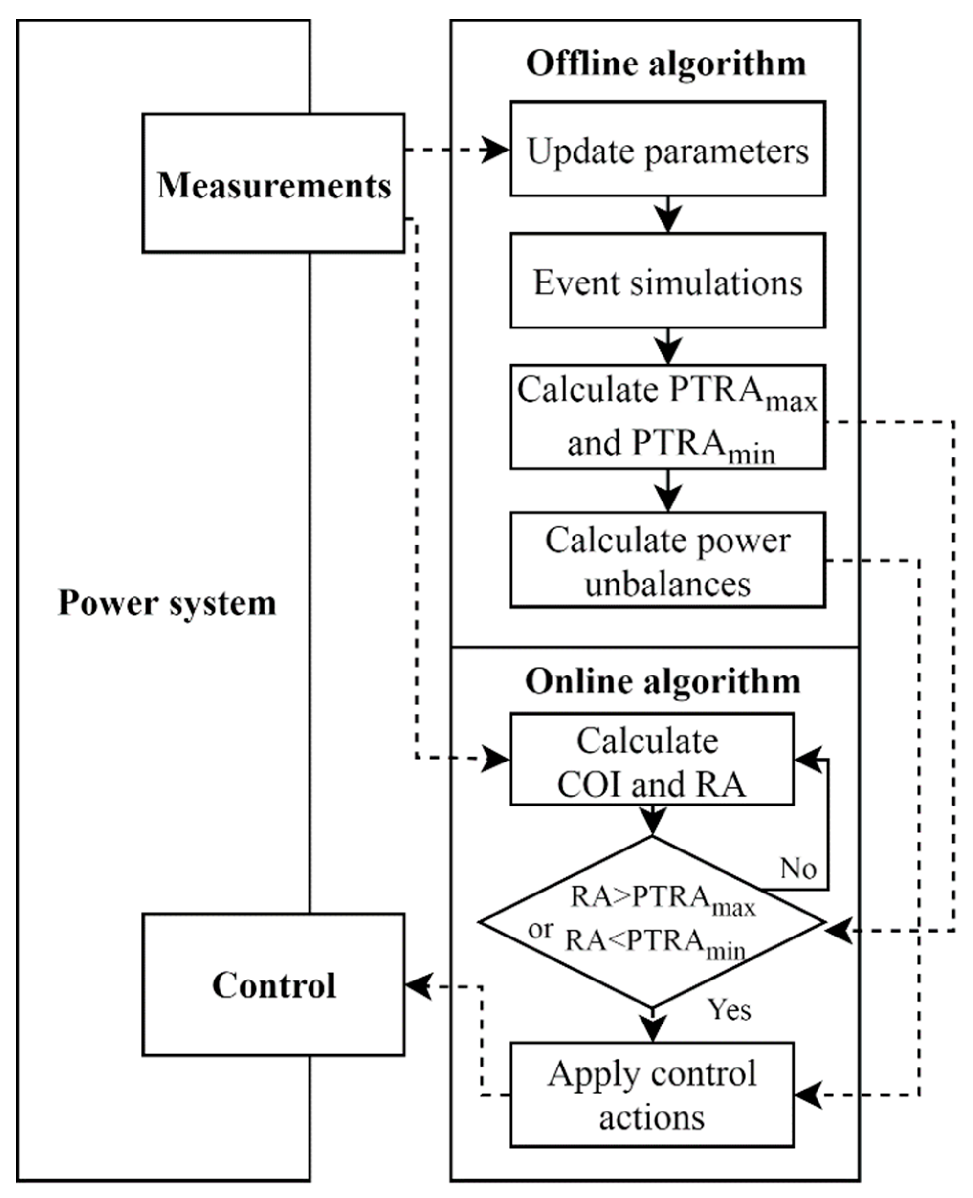
Figure 1 shows the diagram of the methodology applied in this research. The algorithm has two main processes that are conducted for monitoring and predicting transient stability: an offline solution and an online approach. Both processes start reading data from the power system and finish with the applied control to solve the problem detected. Some control actions are applied in this research to demonstrate how the prediction works for the times selected by the algorithm.
2.5. Measurements
Measurements in the power system are carried out with PMUs located in different buses. To perform offline simulation and online monitoring and prediction, PMUs located in the network are divided into two groups and help calculate the parameters and variables needed for the procedure as follows. The first group of PMUs, located in different nodes of the network, helps identify the states of the elements, update the parameters for the offline simulation, and calculate PTRAmax and PTRAmin. The second group of PMUs is located in buses where the COI and RA of generators and areas can be calculated to continuously monitor transient stability and predict oscillations that exceed the limits and become unstable.
2.6. Offline Algorithm
The offline algorithm starts updating the parameters from the power grid through measurements in the power system. Then, offline simulations of different events that represent the risk of operation are performed. PTRAmin and PTRAmax are then calculated through multiple simulations, storing the voltage angles to calculate the relative angle and compare them with the data obtained from the PMUs; thus, with these values, the relative angle and the transient stability can be monitored.
A post-contingency study N-1 is performed by means of dynamic simulations with an equal failure occurrence probability function for all the transmission lines as well as nodal variation of the load. The results are stored in a database considering each simulated scenario to calculate the relative angle at each area, the PTRAmax, and the PTRAmin of the system.
Because this work focuses on a post-contingency wide area study for real-time operation, the proposed analysis only covers a short-term planning horizon and planning and expansion studies are not considered. Thus, the random variables of the power system as the topology of the network must be considered within this planning horizon to reflect in the most real possible way the behavior of the power system. Thus, the following data must be considered in the simulations: faults and transmission line tripping, unit commitment, topology of the network, and load estimation.
Several scenarios, therefore, are proposed for study to ensure the robustness in the database for determining the thresholds. Besides, some required considerations and models are included in the study for more realistic information regarding the post-contingency dynamic response of the power system, such as:
- Changes in power load: based on operating scenarios that consider both increases and decreases in load demand;
- Unit commitment: some independent generators have constant generation;
- Random Probability function PR (5% < PR < 95%) in transmission line faults and short-circuit location. This is used to generate random numbers and simulate the fault distance in transmission lines; and
- Contingency type: changes in the network that result in a topology variation (three-phase faults, fault clearing time, and transmission line tripping).
For each scenario, the power flow was run to identify the operation state. Then, time-domain simulations were performed to determine dynamic post-contingency data and store the results in the database. Because the stability phenomenon considered in this research is short, a time window between six and eight seconds was selected due to the rapid changes presented during the event.
2.7. Online Algorithm
With respect to the online approach, the voltage phase angles obtained from the PMUs are used to calculate the COI and RA in the post-contingency state, which are used to observe and estimate the transient stability of the network and compare with the offline thresholds (PTRAmax and PTRAmin). Then, the system monitors continually if the RA passes the limits with every event presented in the system. When an event is assumed to lead to instability, control actions are performed to prevent this.
2.8. Angle Stability Control
The main objective in the prediction of transient stability behavior is to decide and take early action to prevent loss of synchronism. Further, it aims at continuously monitoring the system in a closed-loop fashion in order to assess whether the control actions have been sufficient or should be reinforced [20]. However, preventive control actions must be added to the preventive control to deal with emergency situations. After critical disturbances studied in this article, the system oscillates and prompt decisions must be considered to maintain power system stability with actions such as generation programming, reactive compensation switching, load shedding, generation trips, shunt compensation switching, and power system separation [21].
The solution presented in this article can be defined as preventive actions that use only time-domain simulation programs and emergency actions with real-time measurements. Then, the power system is continually monitored by using the RA and the thresholds. Thus, if the RA is greater than the maximum value PTRAmax calculated in the offline process, then the angle will increase at a higher rate than the rest of the system and the oscillation will lead to instability; thus, generation must be disconnected from that area. However, if the RA is lower than the minimum value PTRAmin calculated in the offline process, then the angle is decreasing with an area accelerating at a lower rate than the rest of the system and the oscillation will lead to instability; thus the load must be disconnected from the area. The load shedding and generation disconnection are activated once the maximum or minimum value of the PTRA is exceeded. As the main intention of this proposal is not to leave a complete area without electricity service, the generation considered disconnection between 33% and 66% of the maximum generation power at each area when the angle exceeds the PTRAmax. Besides, load shedding was defined as blocks between 20% and 60% of the maximum load associated at each area when the angle exceeds PTRAmin.
3. Results and Analysis
3.1. Case Study on the New England System
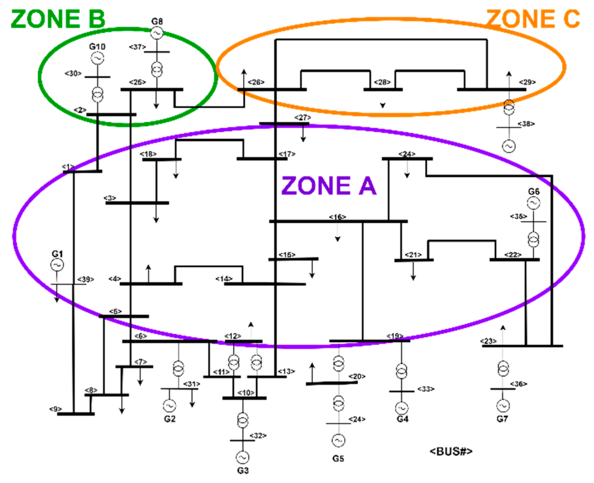
The methodology has been evaluated in the New England 39-bus power system shown in Figure 2. This power system has been slightly modified to satisfy the security N-1 criteria and according to the large number of scenarios considered in the study. This power system has 10 generators, 12 transformers, 46 transmission lines, and 19 loads.
For the transient analysis, we considered simulations between six and eight seconds, each generator represents an area, the voltage angles of the buses are used to calculate the COI and RA that monitor each area, the system has the maximum and minimum PTRA to monitor and predict instability. Transformers next to generation buses were not considered because faults close to the generation plants create a more severe loss of synchronism.
The PMUs were placed in buses where the generation plants were coupled. The PMUs were not located in all buses due to the large amount of data that would be generated and although it was found in several transient stability assessment methods, this was not practical. In addition, it would require a sophisticated communication method for the huge amount of information. In addition, the analysis performed in this research showed that it was not necessary to place PMUs in all the bases where the generation plants were connected because some areas oscillate coherently with others. Figure 2 presents the three zones where different oscillations were found with various simulated faults.
3.2. Minimum and Maximum PTRA
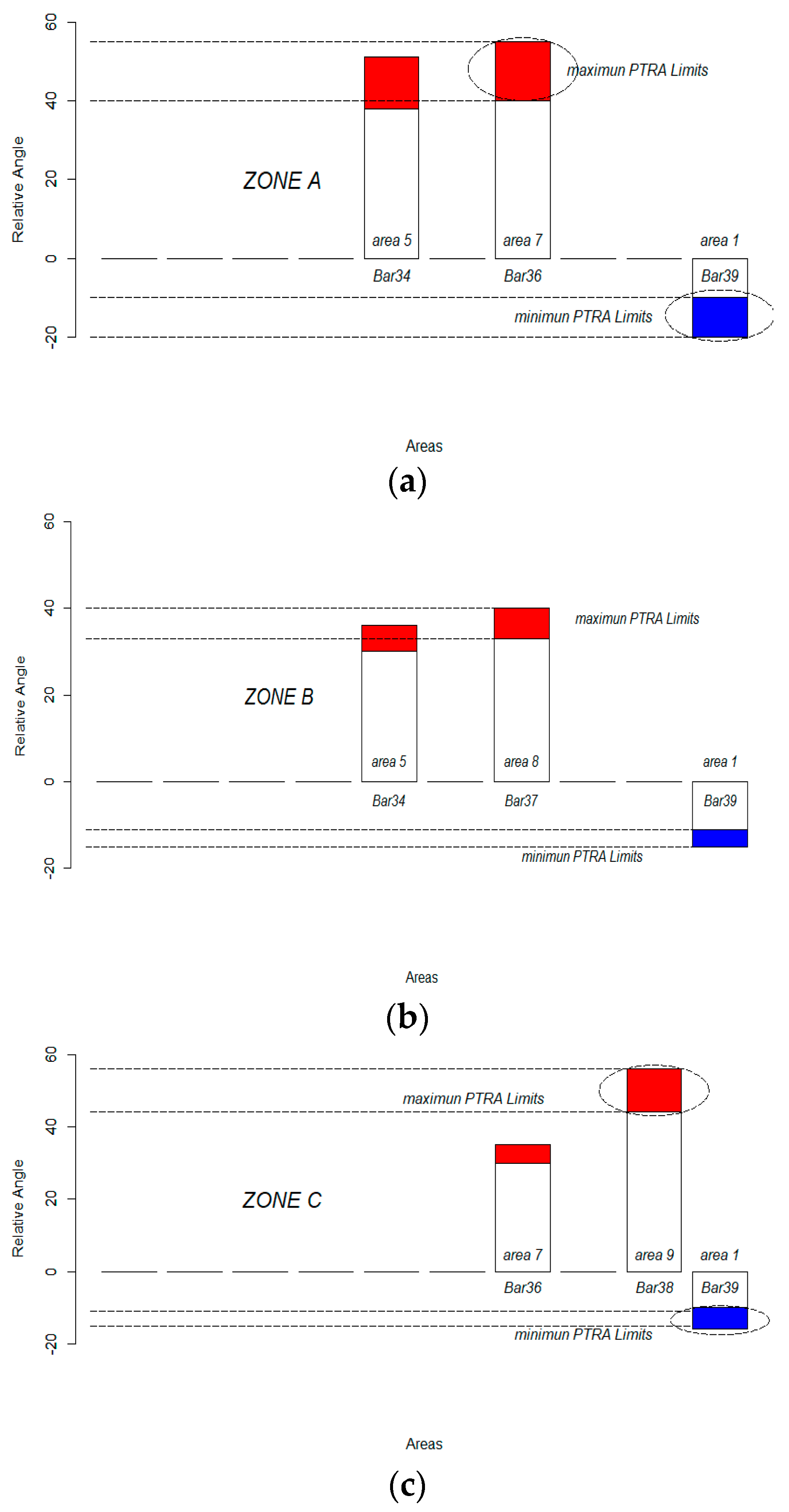
For the calculation of PTRA, post-contingency data were first generated with different scenarios for the dynamic simulation considering various loadability conditions (i.e., load was changed by −5% and +10%), unit commitments (i.e., generation plants with constant power and considering that the load changes), and fault locations. For each scenario, the security of the network during the steady state was previously determined. The simulations were performed with the DIgSILENT POWERFACTORY software, considering three-phase faults, applied randomly in different locations of the power system. The disturbances were performed at each iteration, starting at zero seconds (0 s) until the critical time and the corresponding transmission line tripping. This critical time was different for each scenario. Assuming that the sample time was of 10 milliseconds as the updating time of PMUs and using the voltage phase angle of buses, the COI and RA were calculated for each area in each scenario, constituting a database for the values used to calculate PTRAmax and PTRAmin. Figure 3 shows a summary of the areas where the maximum and minimum thresholds were presented according to the zone of the fault. Figure 3a shows that when the fault occurs in Zone A, a PTRAmax was registered in area 7 with angles between 40° and 55° for most scenarios. In some other scenarios, PTRAmax was reached in area 5 and the angle had similar values to those shown in Figure 3a. Similarly, the PTRAmin was presented in area 1 with angles between −10° and −20°.
When the fault occured in one of the lines associated with Zone B, as shown in Figure 3b, PTRAmax was presented in Area 7 with values between 34° and 40°. Similarly, the minimum angle was presented in Area 1 (PTRAmin) with values between −10° and −15°.
When the contingency is presented in Zone C, the maximum angle (PTRAmax) was presented in Area 9 with values between 40° and 55°. The minimum angle (PTRAmin) was presented in Area 1 with angles between −10° and −15° as shown in Figure 3c.
Few critical contingencies do not allow calculating PTRAmax and PTRAmin when the line was tripped after the fault due to the behavior of the oscillations and loss of synchronism. Those events were presented in the Zone A with the Lines 16-19, 16-21, and 21-22, in Zone B with the Line 2-25, and in Zone C with the Line 28-29.
3.3. Three-Phase Fault
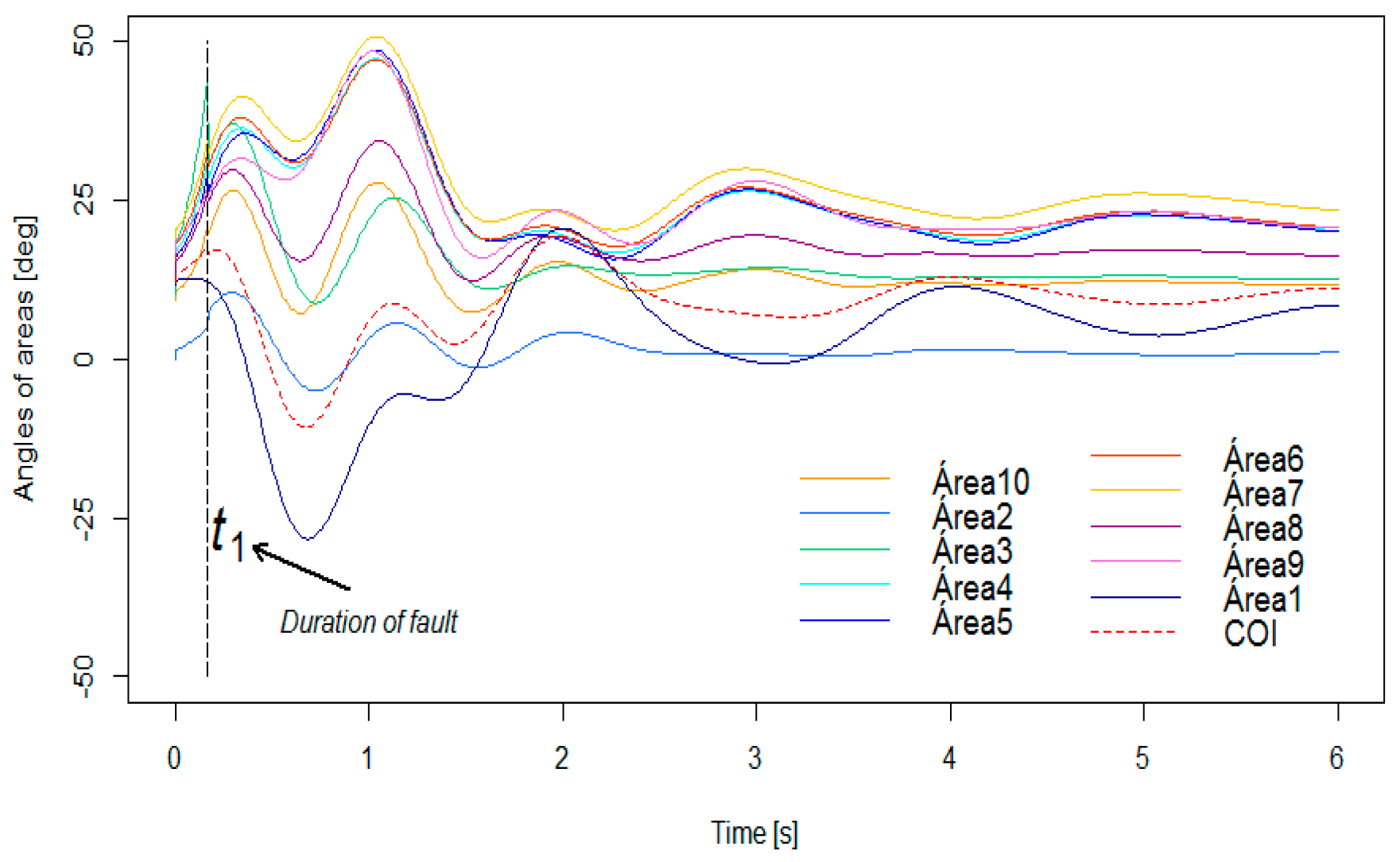
A disturbance in any part of the system will affect the rotor angles of the generators, and thereby, alter the phase angles of the buses. Thus, the fault must be isolated before the critical time for the system to avoid loss of synchronism and to return to an equilibrium point close to the initial conditions. If this condition occurs, then the system remains stable and there is a minimum and maximum angle that the system can reach. Therefore, Figure 4 shows the oscillation of the voltage angles measured at all buses during six seconds after a three-phase fault in Line 4-5 and close to bus 5. For this case, the fault is started at 0 seconds and removed at t1 = 0.17 seconds, which represents the critical fault clearance time.
The power system remains in synchronism after the fault and all areas become stable, returning to equilibrium and close to the initial point. The red dotted line corresponds to the COI, which is the relative oscillation of the power system. Angles of areas show to be coherent and similar to the deviations presented for the COI in the time measured, which is a good indicator of stability. The COI is used to obtain the RA, which is useful to monitor the different areas of the power system. It is important to highlight that the angles shown in Figure 4 are not appropriated to determine a punctual limit due to their oscillations.
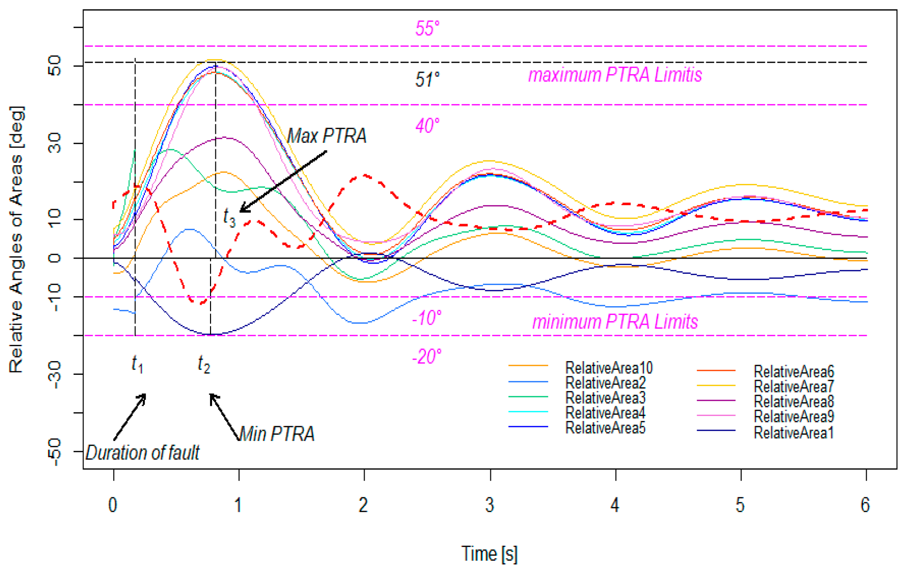
3.4. Relative Angle Calculation
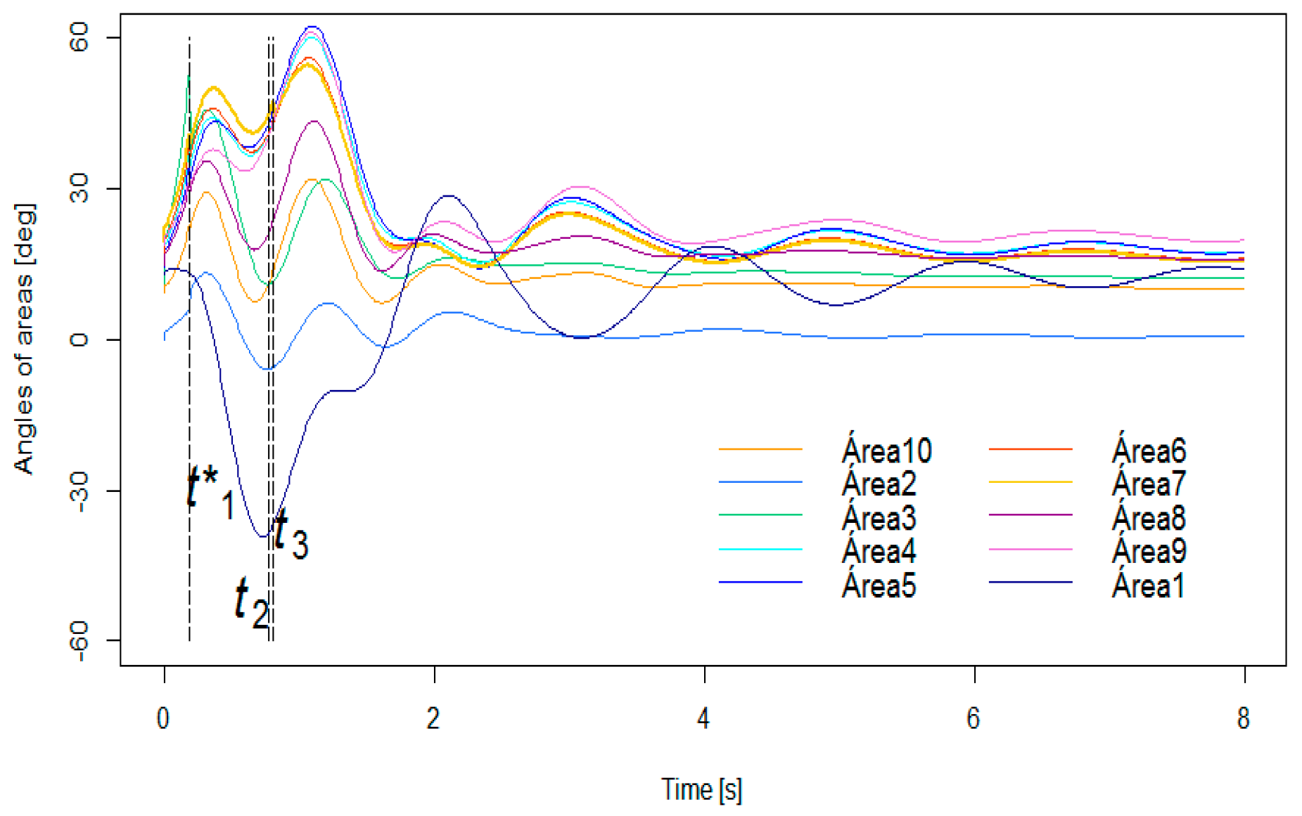
Figure 5 shows the relative angles of each area and the COI (dotted red line) when a three-phase fault is presented in Line 4-5 and cleared after 0.17 seconds (t1); for this case, Generator 2 is the reference machine. Although some areas oscillate in a coherent manner, they are getting away from the system (Areas 4, 5, 6, 7, and 9). Area 7 tends to separate more than the other areas, finding degrees, identified in Figure 4 as t3. In addition, area 1 tends to accelerate at a lower rate than the other areas, thereby slowing down the angle with respect to the oscillation of the system, finding a minimum value of degrees, identified as t2. We have approximated those maximum and minimum threshold values to degrees and degrees, respectively. It was observed that the RA of the areas and maintained inside the critical thresholds (PTRAmax and PTRAmin) and represented in this figure with a dotted fuchsia line.
If a maximum or minimum relative angle threshold is violated, then some control actions can be applied, such as disconnecting generation in the accelerated area in t3 = 0.81 s or load shedding in the decelerated area in t2 = 0.77 s. Those are the predicted times with the transient stability analysis and correspond with an early response to critical events.
In comparison with the angles of the buses (Figure 4), these are opposite to the relative angles (Figure 5), where maximum and minimum limits can be clearly observed in the time. Thus, this demonstrates the advantage of using the COI and RA for a more accurate prediction.
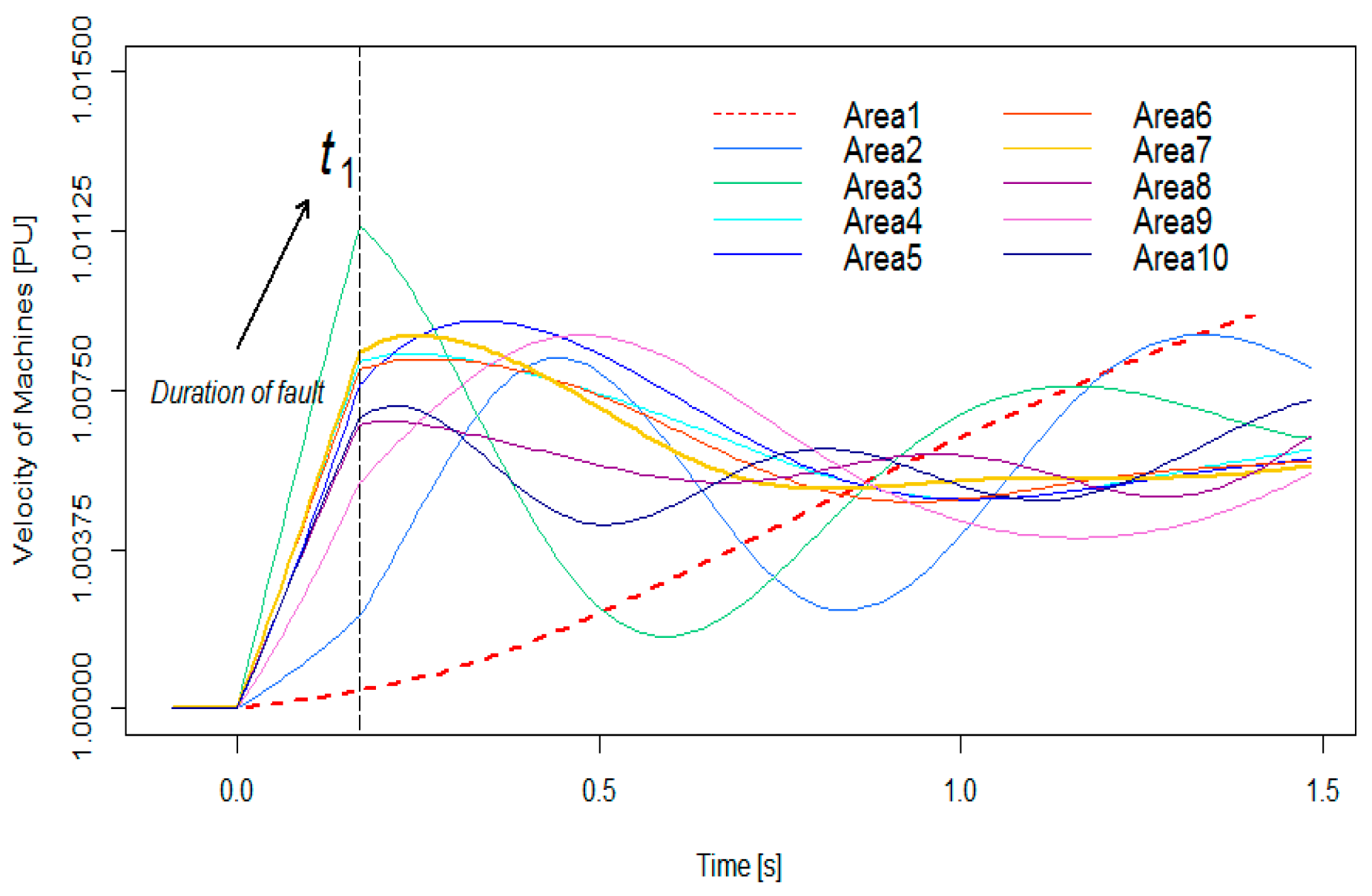
Figure 6 shows the behavior of the power system with the speed of the machines, where Area 1 is accelerating (dotted line). However, the area does not have the same acceleration rate of the other plants and the relative angle moves in the inverse direction of other angles.
For example, when the short circuit occurs in Zone 1, although the mechanical power is higher than the electric power, the rotors of machines in Area 1 accelerate; however, the speed of the reference machine (Area 2) has an acceleration rate greater than the Area 1, and although an accelerating torque is exerted on the shaft of area 1, the angle begins to decrease. With the elimination of the fault, the electric power tries to be equal to the mechanical power, but the rotor continues accelerating because the mechanical power continues being greater than the electrical power and the synchronous speed continues being greater than the rotor speed of Area 1 until Area 1 stores enough kinetic energy and equals the speed of Area 1 and the reference area. Thus, the angle decreases to the minimum point. As mechanical power is greater to the electric power, the angle begins to grow while trying to equal the oscillation of the system.
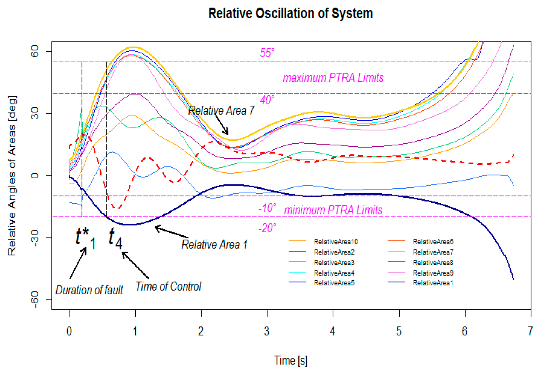
The following scenario shows that after the PTRA is violated, the system suffers a synchronism loss. Thus, Figure 7 shows the computation of the relative angle of each area for a three-phase fault on Line 4-5, close to Bus 5. In this case, the same scenario of Figure 5 is presented, but the PTRA is reached and exceeded; then, the power system was conducted to a loss of synchronism. The fault and the line were removed from the operation at t*1 = 0.19 s, which is greater than the critical time of 0.17 s.
Although the power system attempts to return to an equilibrium point in the stable zone, it fails to maintain the operation, and after some seconds, the operation starts accelerating the generators’ rotor angles. Herein, it is important to highlight that the slopes of the relative angle oscillations are more inclined with respect to the critical time obtained in Figure 5. Thus, the limits and corresponding to the predefined thresholds are violated simultaneously for the oscillation at t4 = 0.56 s, demonstrating that both can be used as indicators to know the events that will end in the unstable zone. Besides, it is important to highlight that a loss of synchronism is presented in this scenario a few seconds after returning to the stability zone, which requires control actions after this condition is predicted.
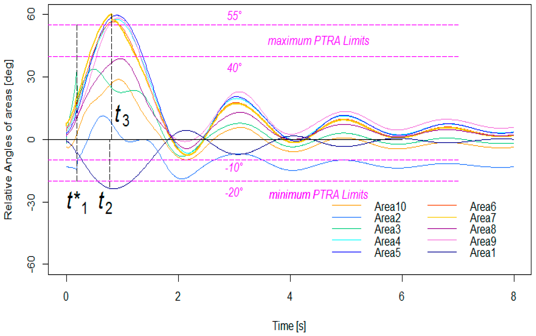
3.5. Control Actions Applied at the Predicted Critical Time
Figure 8 presents the relative oscillation of the areas and Figure 9 shows the voltage angles at buses, when some control actions are applied to maintain synchronism of the power system after a disturbance and based on the prediction of the RA. For this case, the same scenario of Figure 7 is presented, in which a three-phase fault occurs in Line 4-5 and is then removed at t*1 = 0.19 s, and a loss of synchronism of the power system occurs. However, this time, the control action applied with the prediction of the RA helps avoid the loss of synchronism and the power system stabilizes.
When the system violates the limits as in the previous example (Figure 7 at t4 = 0.56 s), the control actions must be achieved such as generation tripping for the accelerated areas and load shedding for the decelerated areas. Therefore, 33% of the generation is disconnected from area 7 (t3 = 0.81 s) at 250 milliseconds after detecting that the angle exceeds the threshold at the equivalent of 15 cycles; besides, 20% of the load is shed from area 1 (t2 = 0.77 s) 210 milliseconds after the PTRAmin is reached, or the equivalent of 13 cycles. The analysis presented in Reference [20], is similar to that obtained in this research, with the difference that in the proposed procedure, load shedding is applied at the time the instability risk is predicted in the minimum relative oscillation angle of the area .
This research shows that one area oscillating in a coherent manner with respect to another with a greater value of RA can be disconnected (Area 5) to avoid a loss of synchronism. In addition, the disconnection of generation in this research is performed with the critical time detected by the maximum threshold and with enough time before loss of synchronism of a machine or area. The research also shows that it is not necessary to disconnect the whole generation of an area or single plant, the actions are just considered for a percentage of generation. Similarly, only a percentage of the load is shed to maintain stability with the generation machines, which accelerate and try to adjust to the relative oscillation of the system, without shedding the complete load.
Table 1 summarizes the results for a three-phase fault on Line 4-5, close to Bus 5. In this table, the term classification represents the two possible conditions: stable 1 and unstable 0. In this scenario, control actions are applied after monitoring the RA with the calculated PTRA. For example, the first case shows that the power system withstands a critical clearance time equal to 0.17 s without control and remains stable: this occurs when the RA remains inside the PTRA. However, for the other two cases presented in Table 1, if the critical clearance time is equal to 0.19 or 0.21 s, then the system becomes unstable: this occurs when the RA gets outside the PTRA. Finally, for the case that the system becomes unstable and some early control actions are required as those used in this study (generation tripping and load shedding), the monitoring and predicting angles with the time shows that by applying control actions at the predicted time the system remains stable. For each area (generation plant), at least three generation units are considered to have enough power to operate and with the possibility of tripping one generation unit (33%) or two generation units for critical cases (66%). Besides, the load may be disconnected in steps of 10% of the total load, up to guarantee the system stability (in the study, a critical event considered a load shedding of 60% of the total load).
Table 2 summarizes the results of some of the simulations performed in this research for different locations of three-phase faults. The term tC is the critical clearance time, GD is the generator to disconnect, %GD is the percentage of the generation to disconnect from an area, tG is the time to disconnect generation, CD is the load to disconnect, %CD is the percentage of load to disconnect from an area, tCa is the time to disconnect load, and tmej is the improved time of the fault.
The fault of each disturbance presented in the table corresponds to the critical time where the system remains stable. In the table, some control actions were considered when the system tended to be unstable, such as generation disconnection or load shedding. These events were controlled by applying power balances to maintain synchronism.
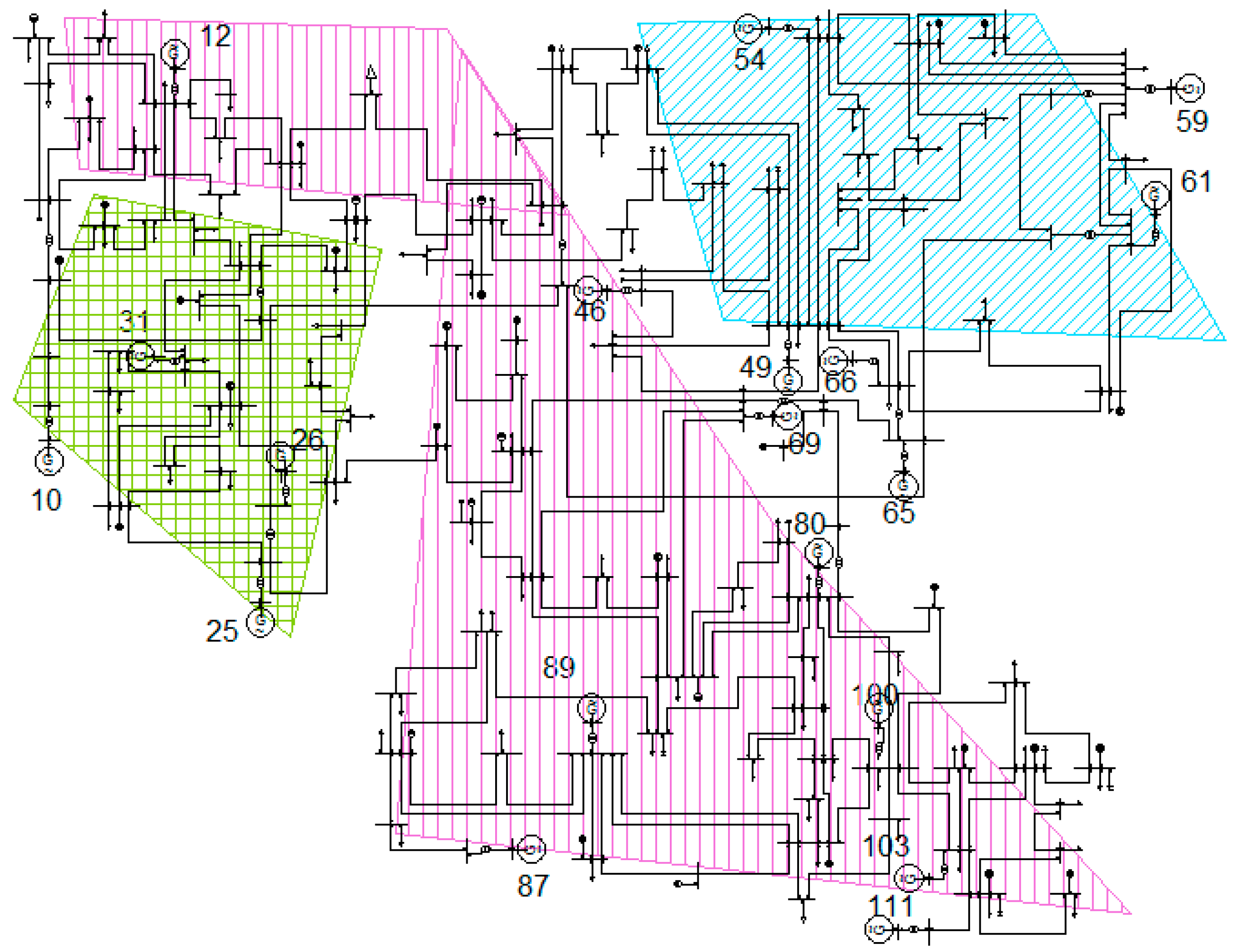
3.6. Case Study on the IEEE 118-Bus Power System
To verify the proposed method, the IEEE 118-bus power system, shown in Figure 10, was used. The test system consists of 54 synchronous machines with IEEE type-1 exciters, 20 of them are synchronous compensators used only to supply reactive power and 15 of them are motors. There are 172 buses, 185 transmission lines, 76 transformers, and 91 constant impedance loads, which consume in total 3668 MW and 1438 MVA [22]. Three-phase faults were considered as contingencies with different clearing time and locations. In the studies, it was assumed that all generators were observable by PMU. Wide-area measurement system (WAMS) were simulated by commercial software that can export the operation states of all generators at every 0.01 s, including voltage angles of buses, rotor angle, rotor speed, electrical power output, and mechanical power output. For this system, a total of 551 simulations were considered, with unit commitment, load changes of −5% and +10%, and random locations of faults in transmission lines with values between 10% and 90% of the line length. Table 3 shows the minimum and maximum PTRA of each zone. As in the previous system, each generation plant represents an area, which is supposed to be composed of three generation units. After analyzing and characterizing the system with its respective oscillations, three zones were found with their respective maximum and minimum relative angles (PTRA).
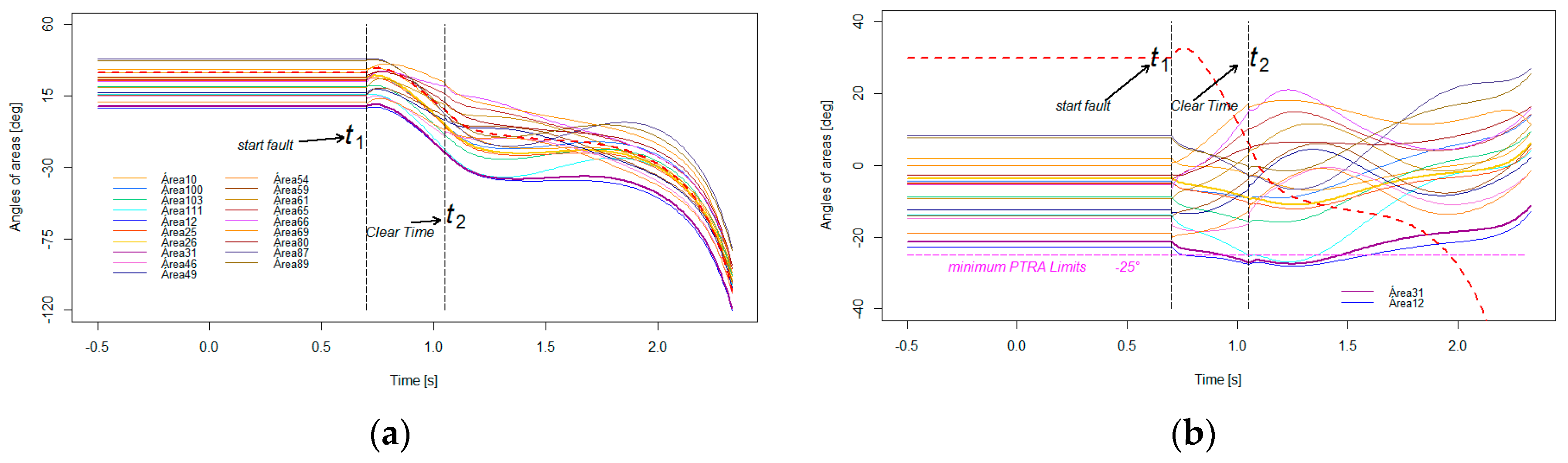
Figure 11a shows the voltage angle curves of each bus where each generation plant was coupled (simulating a PMU), by considering a fault in Line 49-66C1 (Zone B). For this line, the critical clearing time was 300 ms to maintain a stable operation in the post-transient period. In contrast, a three-phase fault was carried out on the same line with starting at 0.7 s (t1) and cleared after 350ms (t2 = 1.05 s). The results show that Areas 31 and 12 exceed the PTRA of Zone B as shown in Figure 11b, and in a second oscillation the system loses synchronism as shown in the voltage angles of buses at each area in Figure 11a.
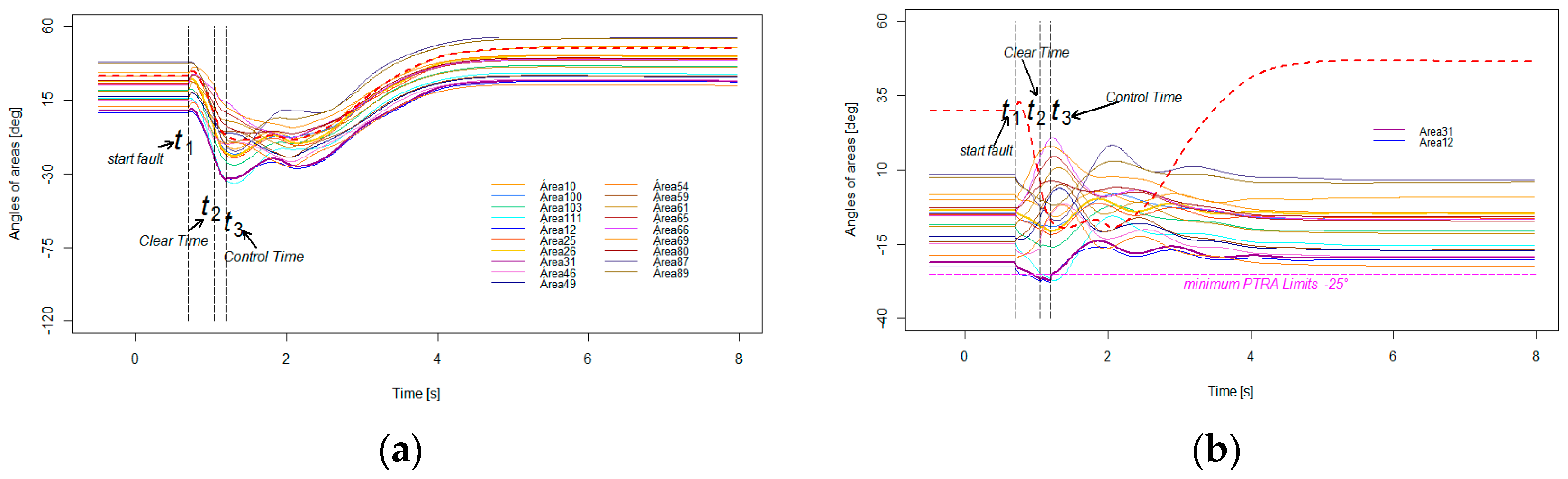
As shown previously, without control actions the system violates the limits even a little before clearing the fault and loses synchronism. Now, the control action executed at t3 = 1.2 s (which considers time delays of communications, as the limit is exceeded 180ms), to avoid the loss of synchronism and to stabilize the system as shows in Figure 12. As Areas 31 and 12 move away by their acceleration rate lower than the rest of areas, then load shedding actions are required to maintain synchronism. Then, only loads in Buses 31, 12, 1, and 11, which are close to the generation areas that exceed the minimum PTRA (Areas 12 and 31), are shed by 50%. It is evident how the proposed method is effective enough to maintain the synchronism of a power system.
4. Conclusions
In this paper, we have demonstrated how the predefined thresholds of relative angles obtained with offline simulations and the relative angles obtained during the online operation with PMUs are very useful to monitor and predict transient stability under real-time operation. All tests were performed on the New England 39-bus and IEEE 118-bus power systems under different contingencies and control actions applied at the predicted time. We obtained that the COI identifies how the generators oscillate with respect to general balance of the power system, identifying the areas that are most close to the loss of synchronism. The RA and the PTRA help monitor and predict instability of the power system with enough time to respond to oscillations.
Furthermore, the simulations indicate the possibility to apply early control actions, such as load shedding or generation tripping, to maintain synchronism conditions in the power grid after faults. All of this is based on data from PMUs. In the implementation conducted, the power system security was improved by early detection of instability and not only by the classical stability criterion acting at the last moment. In addition, the proposed method allows an economic benefit for those generators dispatched at low price in terms of security constraints. The results presented in this paper point to a new way of managing and controlling transient stability based on RAs. In addition, the disconnection of electrical machines with higher RAs is not necessary to prevent power system instability; as a better economic option, other machines with lower RAs, but coherent manner with machines with higher RAs can be disconnected.
In future work, we will endeavor to obtain better indices for monitoring the transient stability and adjusting the control method in order to mitigate the power system oscillations of areas with the minimum power generation or load to disconnect. Our research shows that some buses vary in a coherent manner with very close values; therefore, in future work, it will be useful to propose a methodology to identify and group coherent nodes to reduce the number of PMUs used for obtaining data. On the other hand, it would be appropriate to study the optimal power flow (OPF) that guarantees the best power transfers between areas, in order to decrease angular separations and increase critical clearing times of three-phase faults. Finally, it will be useful to propose algorithms that estimate the operation state as a complement of the data obtained with PMUs and to study the impact of communication delays over RA calculation and control actions.
Author Contributions
Conceptualization, methodology, software, validation, formal analysis, investigation, and writing—original draft preparation, A.F.D.-A. and J.E.C.-B. formal analysis, review and editing, J.F.V.S.
Funding
This research received no external funding.
Acknowledgments
The authors thank the Department of Electrical Engineering and Automation for the valuable support to conduct this research.
Conflicts of Interest
The authors declare no conflict of interest.
References
- Echeverria, D.E.; Rueda, J.L.; Cepeda, J.C.; Colome, D.G.; Erlich, I. Comprehensive approach for prediction and assessment of power system transient stability in real-time. In Proceedings of the IEEE PES ISGT Europe 2013, Lyngby, Denmark, 6–9 Octoberber 2013; pp. 1–5. [Google Scholar]
- Rueda, J.L.; Cepeda, J.C.; Echeverría, D.E.; Colomé, D.G. Real-time transient stability assessment based on centre-of-inertia estimation from phasor measurement unit records. IET Gener. Transm. Distrib. 2014, 8, 1363–1376. [Google Scholar]
- Kundur, P.; Balu, N.J.; Lauby, M.G. Power System Stability and Control; McGraw-Hill: New York, NY, USA, 1994; ISBN 007035958X. [Google Scholar]
- Pai, M.A. Energy Function Analysis for Power System Stability; Springer: Boston, MA, USA, 1989; ISBN 978-1-4612-8903-6. [Google Scholar]
- Farantatos, E.; Huang, R.; Cokkinides, G.J.; Meliopoulos, A.P. A predictive out of step protection scheme based on PMU enabled dynamic state estimation. In Proceedings of the 2011 IEEE Power and Energy Society General Meeting, Detroit, MI, USA, 24–29 July 2011; pp. 1–8. [Google Scholar]
- Aghamohammadi, M.R.; Tabandeh, S.M. A new approach for online coherency identification in power systems based on correlation characteristics of generators rotor oscillations. Int. J. Electr. Power Energy Syst. 2016, 83, 470–484. [Google Scholar] [CrossRef]
- Yan, J.; Liu, C.-C.; Vaidya, U. PMU-Based Monitoring of Rotor Angle Dynamics. IEEE Trans. Power Syst. 2011, 26, 2125–2133. [Google Scholar] [CrossRef]
- Liu, X.D.; Li, Y.; Liu, Z.J.; Huang, Z.G.; Miao, Y.Q.; Jun, Q.; Jiang, Q.Y.; Chen, W.H. A novel fast transient stability prediction method based on PMU. In Proceedings of the 2009 IEEE Power & Energy Society General Meeting, Calgary, AB, Canada, 26–30 July 2009; pp. 1–5. [Google Scholar]
- Karady, G.G.; Gu, J. A hybrid method for generator tripping. In Proceedings of the IEEE Power Engineering Society Summer Meeting, Chicago, IL, USA, 21–25 July 2002; Volume 1, p. 231. [Google Scholar]
- Hazra, J.; Reddi, R.K.; Das, K.; Seetharam, D.P.; Sinha, A.K. Power grid transient stability prediction using wide area synchrophasor measurements. In Proceedings of the 2012 3rd IEEE PES Innovative Smart Grid Technologies Europe (ISGT Europe), Berlin, Germany, 14–17 October 2012; pp. 1–8. [Google Scholar]
- Shi, F.; Zhang, H.; Xue, G. Instability prediction of the inter-connected power grids based on rotor angle measurement. Int. J. Electr. Power Energy Syst. 2017, 88, 21–32. [Google Scholar] [CrossRef]
- Kundur, P.; Paserba, J.; Ajjarapu, V.; Andersson, G.; Bose, A.; Canizares, C.; Hatziargyriou, N.; Hill, D.; Stankovic, A.; Taylor, C.; et al. Definition and Classification of Power System Stability IEEE/CIGRE Joint Task Force on Stability Terms and Definitions. IEEE Trans. Power Syst. 2004, 19, 1387–1401. [Google Scholar]
- Stagg, G.; El-Abiad, A. Computer Methods in Power System Analysis; McGraw-Hill: New York, NY, USA, 1968; pp. 366–397. [Google Scholar]
- Kimbark, E. Power System Stability; Wiley: New York, NY, USA, 1948; Volume 1. [Google Scholar]
- Hashim, H.; Abidin, I.Z.; Yap, K.S.; Musirin, I.; Zulkepali, M.R. Optimization of mechanical input power to synchronous generator based on Transient Stability Center-of-Inertia: COI angle and COI Speed. In Proceedings of the 2011 5th International Power Engineering and Optimization Conference, Shah Alam, Selangor, Malaysia, 6–7 June 2011; pp. 249–254. [Google Scholar]
- Fouad, A.A.; Vittal, V. Power System Transient Stability Analysis Using the Transient Energy Function Method; Prentice Hall: Upper Saddle River, NJ, USA, 1992; ISBN 013682675X. [Google Scholar]
- XM, Direccion planeacion de operación Colombia; CENACE, Direccion de planeamiento y operación Ecuador; CELEC, Centro de operación Ecuador. Generación de seguridad y límites de transferencia de potencia entre los sistemas eléctricos de colombia y ecuador diciembre 2014—diciembre 2015. Technical Report, 2015.
- Ruiz-Vega, D.; Wehenkel, L.; Ernst, D.; Pizano-Martínez, A.; Fuerte-Esquivel, C.R. Power System Transient Stability Preventive and Emergency Control. In Real-Time Stability in Power Systems; Springer: Cham, Switzerland, 2014; pp. 123–158. [Google Scholar] [Green Version]
- Hiskens, I. IEEE PES Task Force on Benchmark Systems for Stability Controls. Technical Report. 2013. Available online: http://www.sel.eesc.usp.br/ieee/IEEE39/New_England_Reduced_Model_(39_bus_system)_MATLAB_study_report.pdf (accessed on 11 February 2019).
- Wahab, N.I.A.; Mohamed, A. Transient stability emergency control of power systems employing UFLS combined with generator tripping method. In Proceedings of the 2010 IEEE International Conference on Power and Energy, Kuala Lumpur, Malaysia, 29 November–1 December 2010; pp. 426–431. [Google Scholar]
- Wehenkel, L. Emergency Control and Its Strategies. In Proceedings of the 13th Power Systems Computation Conference, Trondheim, Norway, 28 June–2 July 1999; Volume 1, pp. 35–48. [Google Scholar]
- IEEE 118-Bus Modified Test System. Available online: http://www.kios.ucy.ac.cy/testsystems/index.php/dynamic-ieee-test-systems/ieee-118-bus-modified-test-system (accessed on 11 February 2019).
Figure 1.
Flowchart of the algorithms to predict transient stability.

Figure 2.
New England 39-bus system.

Figure 3.
Evaluation of fault events in the three zones: (a) Zone A, (b) Zone B, and (c) Zone C.

Figure 4.
Voltage angles measured in the generation buses after fault clearance at 0.17 s.

Figure 5.
Relative oscillation of the power system for a three-phase fault in Line 4-5 cleared at 0.17 s.
Figure 5.
Relative oscillation of the power system for a three-phase fault in Line 4-5 cleared at 0.17 s.

Figure 6.
Speed of the machines for a three-phase fault in Line 4-5 and cleared at 0.17 s.

Figure 7.
Relative oscillation of the power system for a three-phase fault in Line 4-5 cleared at 0.19 s.
Figure 7.
Relative oscillation of the power system for a three-phase fault in Line 4-5 cleared at 0.19 s.

Figure 8.
Relative oscillation of the power system for a three-phase fault in Line 4-5 cleared at 0.19 s and with some control actions applied.
Figure 8.
Relative oscillation of the power system for a three-phase fault in Line 4-5 cleared at 0.19 s and with some control actions applied.

Figure 9.
Voltage angles at buses when a fault occurs at 0.19 s in Line 4-5 and some control actions are applied.
Figure 9.
Voltage angles at buses when a fault occurs at 0.19 s in Line 4-5 and some control actions are applied.

Figure 10.
IEEE 118-bus power system [22].
Figure 10.
IEEE 118-bus power system [22].

Figure 11.
Angles measured in the generation buses of the IEEE 118-bus power system after a three-phase fault in Line 49-66C1 with clearing time at 0.350 ms. (a) Voltage angles and (b) relative angles.
Figure 11.
Angles measured in the generation buses of the IEEE 118-bus power system after a three-phase fault in Line 49-66C1 with clearing time at 0.350 ms. (a) Voltage angles and (b) relative angles.

Figure 12.
Angles measured in the generation buses of the IEEE 118-bus power system after a three-phase fault in Line 49-66C1 with clearing time at 0.350 ms and control actions such as generation tripping and load shedding. (a) Voltage angles and (b) relative angles.
Figure 12.
Angles measured in the generation buses of the IEEE 118-bus power system after a three-phase fault in Line 49-66C1 with clearing time at 0.350 ms and control actions such as generation tripping and load shedding. (a) Voltage angles and (b) relative angles.


Table 1.
Results for the fault in Line 4-5.
| Fault Duration (s) | 0.17 | 0.19 | 0.21 | |||
|---|---|---|---|---|---|---|
| Area | 1 | 7 | 1 | 7 | 1 | 7 |
| Classification | 1 | 1 | 0 | 0 | 0 | 0 |
| Generation Disconnection | - | - | - | 33% | - | 66% |
| Load Shedding | - | - | 20% | - | 20% | - |
| Time for Control | - | - | 0.77 | 0.81 | 0.77 | 0.81 |
Table 2.
Transient stability prediction with relative angles for different faults.
| Faulty Lines | Lines Disconnected | tC | GD | %GD | tG | CD | %CD | tCa | tmej |
|---|---|---|---|---|---|---|---|---|---|
| 4-14 (5%) | 4-14 | 0.17 | 7 | 66 | 0.65 | 1 | 30 | 0.79 | 0.2 |
| 4-14 (95%) | 4-14 | 0.17 | 7 | 33 | 0.78 | 1 | 50 | 0.84 | 0.19 |
| 5-6 (5%) | 5-6 | 0.19 | 7 | 33 | 0.82 | 1 | 50 | 0.82 | 0.21 |
| 5-6 (95%) | 5-6 | 0.18 | 7 | 33 | 0.82 | 1 | 20 | 0.82 | 0.2 |
| 16-21 (5%) | - | 0.1 | 7 | 33 | 0.38 | 1 | 60 | 0.8 | 0.12 |
| 16-21 (95%) | - | 0.13 | 7 | 66 | 0.34 | 1 | 20 | 0.77 | 0.16 |
| 2-25 (5%) | - | 0.15 | 5 | 33 | 0.9 | 1 | 20 | 0.79 | 0.17 |
| 2-25 (95%) | - | 0.16 | 5 | 66 | 0.74 | 1 | 20 | 0.74 | 0.21 |
| 4-5 (5%) | 4-5 | 0.16 | 5 | 66 | 0.75 | 1 | 40 | 0.75 | 0.21 |
Table 3.
Limits of fault events in the three zones.
| Items | Zone A | Zone B | Zone C |
|---|---|---|---|
| Area (Generators) | 10 and 25 | 31 and 12 | 49 |
| PTRA | 29° | −25° | 28 |
© 2019 by the authors. Licensee MDPI, Basel, Switzerland. This article is an open access article distributed under the terms and conditions of the Creative Commons Attribution (CC BY) license (http://creativecommons.org/licenses/by/4.0/).
Share and Cite
MDPI and ACS Style
Diaz-Alzate, A.F.; Candelo-Becerra, J.E.; Villa Sierra, J.F. Transient Stability Prediction for Real-Time Operation by Monitoring the Relative Angle with Predefined Thresholds. Energies 2019, 12, 838. https://doi.org/10.3390/en12050838
AMA Style
Diaz-Alzate AF, Candelo-Becerra JE, Villa Sierra JF. Transient Stability Prediction for Real-Time Operation by Monitoring the Relative Angle with Predefined Thresholds. Energies. 2019; 12(5):838. https://doi.org/10.3390/en12050838
Chicago/Turabian StyleDiaz-Alzate, A. F., John E. Candelo-Becerra, and Juan F. Villa Sierra. 2019. "Transient Stability Prediction for Real-Time Operation by Monitoring the Relative Angle with Predefined Thresholds" Energies 12, no. 5: 838. https://doi.org/10.3390/en12050838
Note that from the first issue of 2016, this journal uses article numbers instead of page numbers. See further details here.