Reuse of Data Center Waste Heat in Nearby Neighborhoods: A Neural Networks-Based Prediction Model

Abstract

This paper addresses the problem of data centers’ cost efficiency considering the potential of reusing the generated heat in district heating networks. We started by analyzing the requirements and heat reuse potential of a high performance computing data center and then we had defined a heat reuse model which simulates the thermodynamic processes from the server room. This allows estimating by means of Computational Fluid Dynamics simulations the temperature of the hot air recovered by the heat pumps from the server room allowing them to operate more efficiently. To address the time and space complexity at run-time we have defined a Multi-Layer Perceptron neural network infrastructure to predict the hot air temperature distribution in the server room from the training data generated by means of simulations. For testing purposes, we have modeled a virtual server room having a volume of 48 m³ and two typical 42U racks. The results show that using our model the heat distribution in the server room can be predicted with an error less than 1 °C allowing data centers to accurately estimate in advance the amount of waste heat to be reused and the efficiency of heat pump operation.

1. Introduction

Nowadays data centers (DCs) are subjected to significant pressure to perform more efficiently from an environmental perspective towards generating carbon-neutral benefits. The DC industry is investing in finding effective ways to improve energy efficiency. The challenge is how to turn the environmental focus into a long-term business opportunity by finding new revenue streams. The electricity consumed by the IT infrastructure to implement the DCs’ core mission, which is to reliably execute their clients’ workload, is almost completely converted into heat. Additionally, even in well designed DCs, the cooling system consumes almost 37% of the total energy demand to maintain the temperature set points for the servers’ safety [1]. The H2020 CATALYST project [2] vision is to achieve cost and environmental efficiency by integrating DCs with the districting heating infrastructure transforming them into active players in the thermal energy value chain.

Naturally, in this context solutions for re-using the otherwise wasted heat of a DC in nearby neighborhoods have been proposed, however, even though there is a big potential for DC heat reuse there are still technological challenges that need to be addressed. The first challenge is the low quality of waste heat extracted from DC, while the second one is the efficiency in the operation of the heat pumps [3]. This is, in particular, true for air-cooled DCs using electrical cooling systems where the heat extracted from the server rooms has a temperature below 40 °C [4]. To make heat usable and marketable the DCs have to install heat pumps that are able to raise heat temperature to around 80 °C which allows heat transportation over longer distances to nearby buildings [5]. In the latter case, the heat pump consumes energy in the process of increasing heat quality [6]. The more efficient a heat pump is, the less energy it will consume and it will be more cost-effective for a DC to operate it. One of the factors influencing this is air temperature in the server room. The higher the temperature the less energy the heat pump will consume. Thus, methods for increasing the server room temperature set points have emerged allowing the temperature of the air extracted in the server room to increase. However, this leads to the third issue related to the generation of server room hotspots, that can lead to emergency stops or server failure. To avoid such hazardous situations, the server room and cooling system settings and configurations need to be properly evaluated by simulations allowing the DC operators to properly assess their impact in terms of heat distribution, prior of making them effective. We address the above-presented issues by bringing the following novel contributions:

• Definition of a heat reuse model for DCs allowing them to estimate in advanced the amount of generated waste heat and the impact on the efficiency of the heat pump operation;
• Definition of Computational Fluid Dynamics (CFD) models to simulate the thermodynamic processes inside the server room and estimate the temperature of the hot air generated;
• Development of neural networks algorithm to predict the heat distribution in the server room from training data generated using the CFD simulations, making our model feasible for near real-time decision making;

By using the proposed approach, the DC operators will be able to accurately forecast the temperature of the hot air recovered from the server room and the amount of waste heat that might be reused. They will also be able to compare and contrast additional investment costs with incremental revenues that can be achieved from valorizing forecasted waste heat.

The rest of the paper is organized as follows: Section 2 describes the relevant related work in the area of DC heat grid integration focusing on the approaches for modeling the thermal processes and predicting the heat distribution inside the server room. Section 3 presents an analysis of the heat reuse potential of the Poznan Supercomputing and Networking Center (PSNC) Section 4 details our proposed DC waste heat reuse model which combines the Computational Fluid Dynamics with neural network based prediction infrastructure and Section 5 presents evaluation results for a virtual server room with two racks. Section 6 concludes the paper and presents suggestions for relevant future work.

2. Related Work

Several solutions proposed in the literature tackle the reutilization of DCs’ waste heat for heating-up closely located houses, apartments and offices [6,7,8]. District heating (DH) networks, already identified as an important need the intelligent heat distribution process that must take advantage of the third party-generated heat (DCs are candidates for this process) [9]. Other approaches are aimed at providing heat-oriented ancillary services which involve forecasting methods to identify heat demand patterns [10,11]. Modeling and simulation techniques are defined in [12,13] with the objective of reusing and transporting thermal energy within DH networks. These can help to evaluate limitations, benefits, and costs and serve as a preliminary feasibility study before actual solution implementation. Another aspect to be considered is the reduction of emissions generated for peak load production of thermal energy usually produced with fossil fuels [2].

In the direction of DCs integration with heat networks, modeling thermal processes related to the computing infrastructure and discovering their impact on the surrounding environment has recently gained in popularity. A constant increase in spatial and thermal density of computing systems make their evaluation more important but also more challenging. For now, Computational Fluid Dynamics (CFD) simulations are seen as the most suitable solution. In contrast to experimental examinations, CFD allows obtaining the volumetric field of many physical variables. It is also much more convenient and cheaper to simulate varying scenarios than evaluate them in the real world. Numerous examples of studies of airflow inside the server room with CFD analysis can be found in the literature. A detailed CFD analysis of various air distribution systems and their cooling efficiency was described in [14], while in [15] the impact of air conditioning failures and fluctuations of servers’ power were considered. Other studies [16] were focused on the analysis of optimal airflow angle through supply tiles for server rooms with raised floor cooling system. Nevertheless, the CFD-based solutions are effort-intensive for model preparation and time consuming for gaining good results, which makes them inadequate for complex system simulations and analysis of numerous configurations. As an alternative, the Potential Flow Model [17] and orthogonal decomposition methodology [18] have been proposed to reduce the complexity of the initial CFD model. Another approach is leveraging on analytical models which are applied directly within the process of DC thermal evaluation or to the simulation toolkits. The power and thermal models proposed in literature correspond to different levels in the hierarchy of resources within DC. In [19] the authors discussed the power models of a server and its subcomponents, while the thermal behavior of a server is analyzed in [20]. The models define the temperature of the processing unit, as well as the changes in the temperature at the server’s outlet. Extension to these models, including the power leakage phenomena is described in [21]. Moreover, in [20] also the power models for the whole data center are proposed, together with the corresponding cooling models [22]. A simplified version of the cooling model was presented [23], while [24] introduced the concept of a heat distribution matrix specifying the heat recirculation between the servers. It defines the impact of hot air leaving the server to its inlet. Authors showed also how a combination of CFD simulation, together with a heat flow model and analytical data can contribute to the overall thermal analysis of a DC. An example of the complex simulation environment for the assessment of DC energy and thermal efficiency is the SVD Toolkit being, the result of the CoolEmAll project [25]. The toolkit integrates analytical simulations and the CFD modeling to the impact of different DC’s management policies, hardware configurations and intensity of workloads. In this way, it enables energy-efficiency and heat-efficiency optimization with respect to the common metrics.

However, to perform a complex evaluation of the DC, including analysis of the great number of possible states and with plenty of parameters, another approach, which benefits from the aforementioned solutions, is required. Thus, in this paper, we built upon the existing state of the art to present a combination of CFD simulations with a neural network-based prediction infrastructure to allow the forecast of temperature distributions in server rooms considering a high number of different cases. Our approach is rolling in the black-box prediction methodologies which allow for learning a prediction model at of training data without any information on the underlying physical processes. The prediction model, once learned, features low computational and time overhead, and could be integrated with a proactive DC management strategy to control workload allocation and cooling system settings for adapting the DC heat generation in order to meet different heating goals [1].

Few learning-based approaches are described in the research literature. In [26,27] such algorithms are trained to predict the behavior of the DC cooling system. In [27] data measured from a real DC is used for training a feedforward and a dynamic recurrent artificial neural network and results are compared against a CFD simulation. The proposed system has comparable accuracy with the CFD simulation but a much faster convergence time and can be incorporated in real-time control strategies. Similarly, in [28], a neural network solution is proposed for predicting DC temperatures. The neural network approach has the advantage that it can learn the environment continuously by adapting its parameters each time new environment data is taken from sensors. The neural network can be initially trained either with real environmental data or with data generated by a CFD simulation for the DC model. In [29] a novel thermal forecasting method is developed which can predict server temperatures using data streams acquired from sensors. Compared with CFD-based solutions the proposed one is simpler and uses a gray-box model of the underlying physical systems to model the thermodynamic processes and sensor data together with an algorithm that continuously adapts the models to new monitored data. Evaluation results show better prediction accuracy than standard approaches driven only by data and identifying risky situation 4 minutes before they appear. Similarly in [30] the authors use the trained model as input to a thermal-aware scheduling algorithm and evaluated its performance through simulations.

3. PSNC Data Centre Example

The DC IT infrastructure executes the clients’ workload and as result, heat is generated and it accumulates in the server room. All consumed electricity of DC IT infrastructure is ultimately converted into heat that needs to be dissipated by an electrical cooling system in order to maintain the temperature inside the server room under pre-defined set points for safe operation of servers. As the IT servers design is continuously improved for operating at higher temperatures and the server room density continues to rise, the DCs will become important producers of waste heat.

One of such DC is the PSNC [31] which already uses part of the heat produced by its DC to provide heating for offices (for around 300 people) located within the same building. PSNC is located nearby a campus of the Poznan University of Technology (PUT) so further potential use of the remaining waste heat was identified. Analysis of this case provides motivation and requirements for the models and methods of heat reuse prediction and optimization proposed in this paper.

3.1. Heat Reuse Within the Building

PSNC’s DC covers an area of 1600 m² with a maximum (possible) power capacity equal to 2 MW (and with the possibility to extend the supplied power up to 16 MW). However, the usual, average power drawn by DC is around 0.9 MW. IT infrastructure is both liquid and air-cooled (where the liquid cooling is used for the HPC part of the DC) resulting in a Power Usage Effectiveness (PUE) of 1.3. Currently, around 400 kW is used by the system using a Direct Liquid Cooling (DLC) approach. Shortly, the DC will be extended by another DLC system leading to an increase the mean power usage (>1 MW). The average resource usage oscillates around 70%, however, the utilization of nodes of the largest HPC system reaches often 90%. In the liquid cooling system, the inlet/outlet temperatures of the coolant are up to 35/45°C in the summer and 20/30 °C, respectively, in the rest (around 70%) of the year. 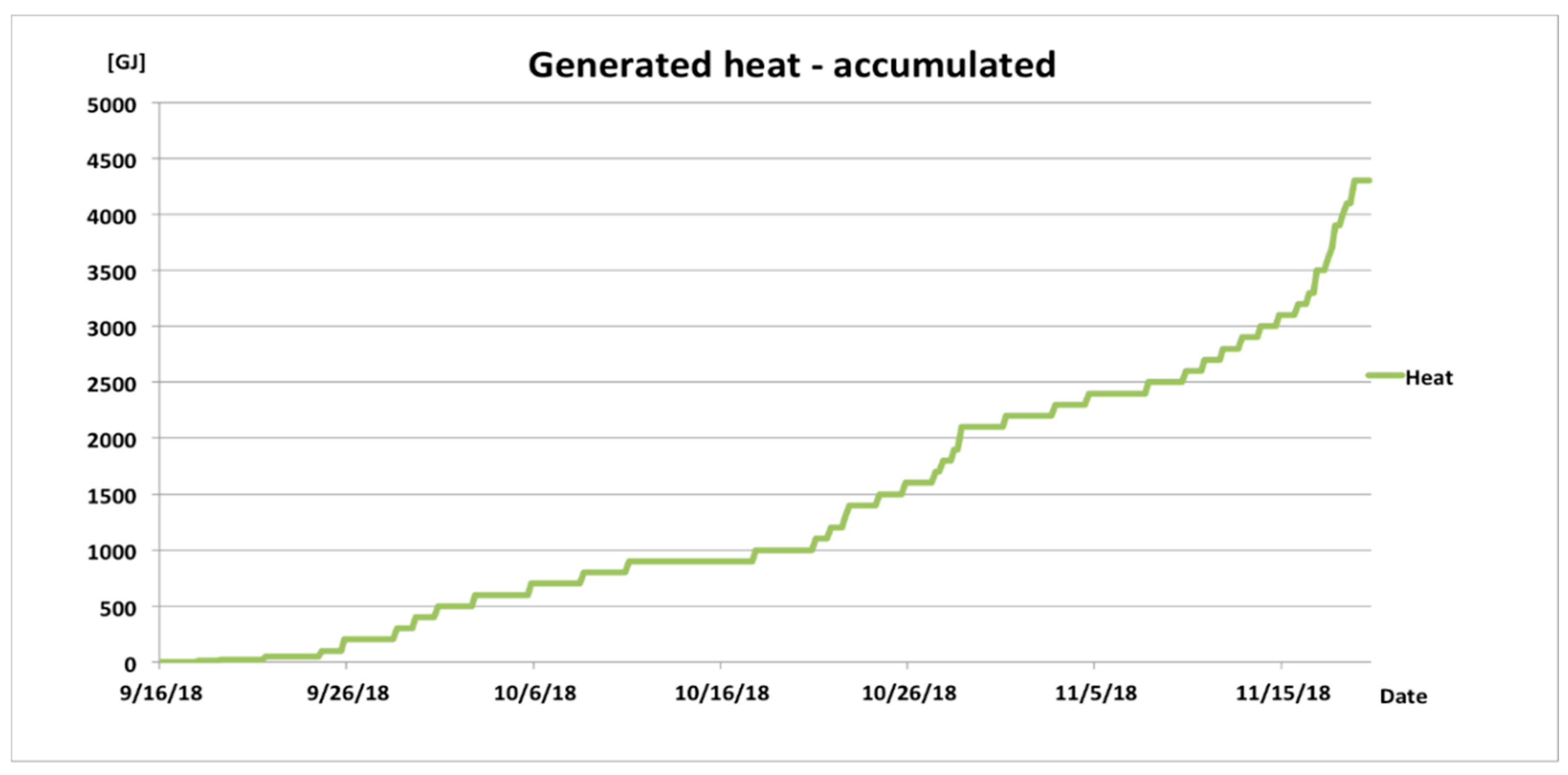Figure 1 shows the amount of accumulated heat, generated in DC within the period of two months between September and November.

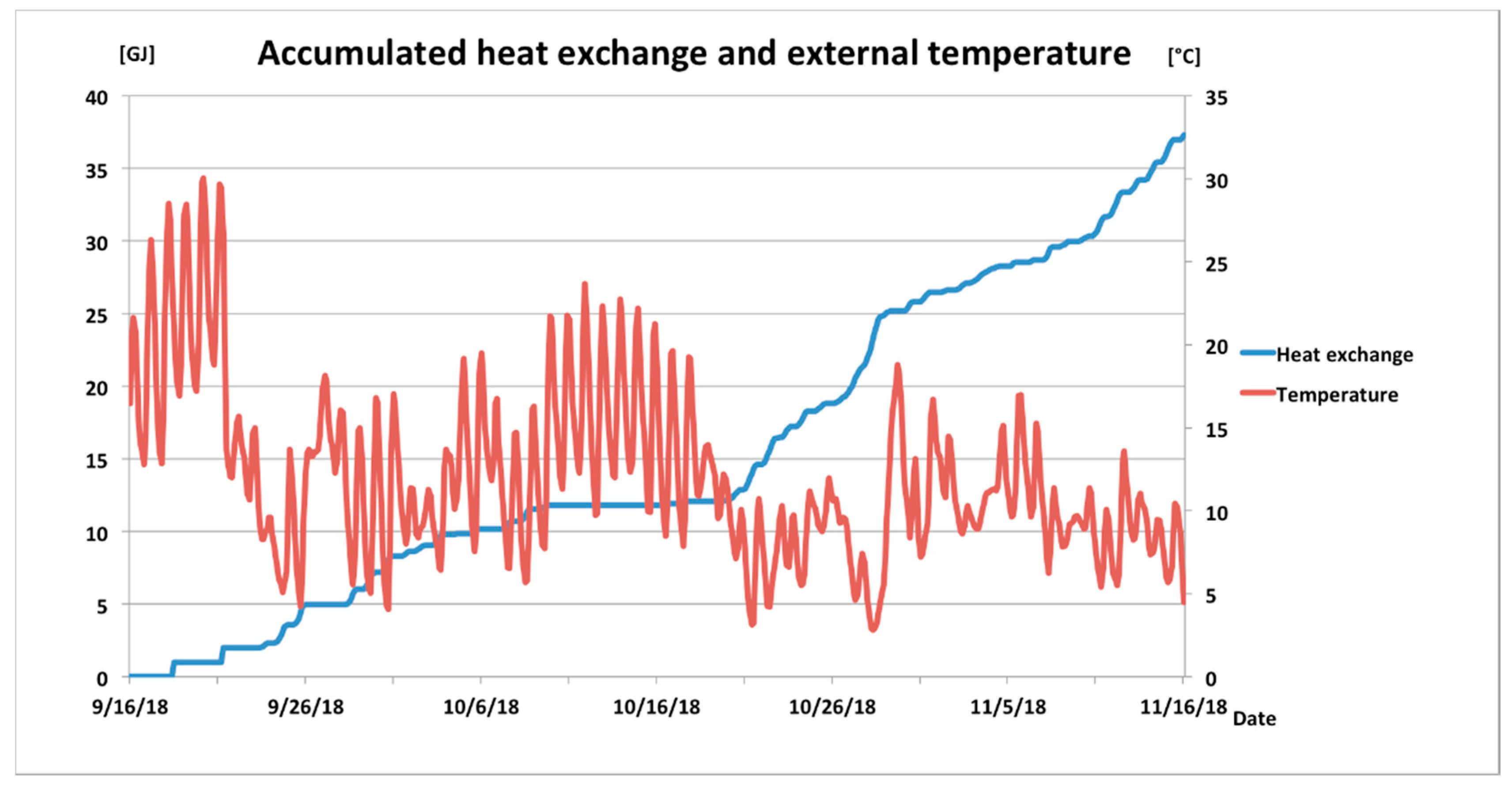
One should note that the total increase in the amount of heat within the evaluated period was around 4200 GJ, which corresponds to the average power drawn by the DC. Currently, the heat from DC is used for heating the whole PSNC building. PSNC’s facilities are equipped with a 300 kW heat exchanger. The total heat reused is within 200–300 kW in the winter season. The heat is reused from both low and high-temperature loops. The following chart (Figure 2) shows the heat supplied (from the DC) to the PSNC building and the external temperature characteristics within the evaluated time slot.

Also, the more rapid increases in the amount of heat exchanged correspond the drops in the external temperatures. The total amount of heat exchanged in the analyzed period was around 40 GJ, which is far below the capabilities of the current heat exchanger.

3.2. Heat Reuse in the Nearby Neighbourhood

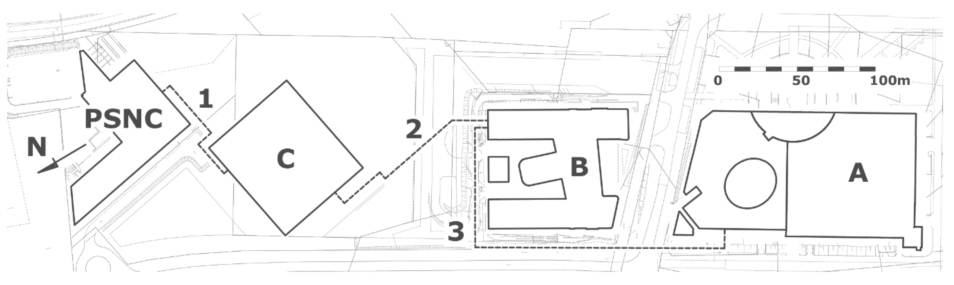
In the neighborhood of the PSNC building, there is a PUT campus. The PSNC building is thus located near three main buildings: the Faculties of Architecture and Engineering Management Building (building C), Faculty of Chemical Technology Building (building B) and Library and Lecture Center Building (building A), all only at most 400 meters away. This can be seen in Figure 3. Buildings A and B are equipped with air cooled water chillers and coupled with heating substations connected to the Poznan district heating network, with a contracted power demand of 1027 kW and 500 kW respectively. Building B is also equipped with 360 kW heating power Ground Source Heat Pumps (GSHPs). In building C, a nearly zero-energy one, cooling and space heating is provided by a low temperature thermally activated building system and heat is generated only with the GSHPs.

Heating energy demand is covered with the use of GSHP by 100% for building C and by 80% for building B. Heat generated with GSHPs costs 10 €/GJ, while heat from the district heating network costs twice this price. 100% of the heating energy for building A (5430 GJ annually) and 20% for building B (843 GJ annually) is provided by heating substations, resulting in a total of 6273 GJ annually.

A water loop of 250 kW and 5 °C supply/return temperature difference between buildings B and C was designed, as both B heating station and water chillers are oversized. Two operating modes are considered:

• Heat peak source for building C—building C heating system is assisted with heat from building B during winter;
• Building C cooling—chilled water from building B chillers and heat pumps is supplied to building C cooling system.

A detailed design for the water loop was prepared and it is to be built in the first half of 2019 when building C will be put into use.

As the heat production of PSNC exceeds its energy need subsequent considerations on capabilities of heat transfer between PSNC and PUT buildings were conducted. It was assumed that 700 or up to 1000 kW heat could be transferred to buildings B and C. Two subsequent water loops between PSNC and building C and between buildings A and B should be built together with local storage tanks and pumping stations (Figure 4).

Supply/return water temperature for building B heating system is 60/45 °C and 80/60 °C for building A, built earlier with less thermal protection. Building C heating system with a thermally activated building system is a very low-temperature one with temperatures of 35/30 °C.

PSNC utilizes DC waste heat with a local multi-split and variable refrigerant volume systems. Water-to-water or air-to-water heat pump should be used in PSNC to increase the temperature of air or chilled water returning from the DC to slightly above the building supply temperatures to thus cover the heat losses in water loops and in the heat exchangers in each building. Exchangers are necessary to separate the water systems. To obtain higher supply temperatures additional boilers or second heat pump could be used in a particular building. The total length of the loop, made with pre-insulated pipes, will be less than 500 m.

Taking into account the current heat demands of the PSNC building and the upcoming enlargement of the DC’s computational capabilities, there are promising prospect to fulfill the PUT heat demands at least partially by using the PSNC facilities. However, the heat demand of the neighborhood may vary significantly depending on external temperatures. Additionally, DC heat generation and outlet temperatures may differ depending on load, temperatures, and cooling system configuration. Therefore, the optimal configuration of such a system requires accurate prediction of heat production and the state of the system. Models and methods for such accurate prediction of the DC thermal flexibility are studied in the following sections.

4. Optimizing DC Heat Reuse

4.1. Heat Energy Harvesting Efficieny

The potential value of residual heat is partially determined by applied cooling technology from where the energy has been gathered. The heat produced by the servers has low temperature, due to the low temperature range of their safe operation (T_HOTAIR ≤ 30 degrees Celsius) but at the same time it is the simplest and most efficient method to recover the waste heat and reuse it for domestic heating. However, district heating networks usually require temperatures above 60–70 degrees Celsius. The thermal energy must either be harvested at a higher temperature; this being possible only for liquid cooling systems (that can reach a temperature of 60 degrees Celsius) or passed through a heat pump to increase its temperature ($T_{DISTRICT}$) by using a refrigerant cycle that consumes electrical energy. Consequently, DCs that rely mostly on air cooling systems are equipped with heat pumps to raise the temperature of the reused heat.

The heat pump has two coefficients of performance indicators (COP): one defined for the cooling process of the air to be fed back to the DC server room through the perforated floor and one defined for the heating process to deliver in nearby neighborhoods:

$$CO{P}_{Cooling}=\frac{∆Q_{Cool}}{E_{Compressor}}\le \frac{T_{COLDAIR}}{T_{HOTAIR}-T_{COLDAIR}}$$

(1)

$$CO{P}_{Heating}=\frac{D{Q}_{Hot}}{E_{Compressor}}\le \frac{T_{DISTRICT}}{T_{DISTRICT}-T_{HOTAIR}}$$

(2)

where $E_{Compressor}$ is the heat pump compressor energy consumption. In other words $CO{P}_{cooling}$ characterizes the process done by the pump to cool the server room, while $CO{P}_{Heating}$ characterizes the process done by the heat pump to increase temperature of supplied heat and to transfer it.

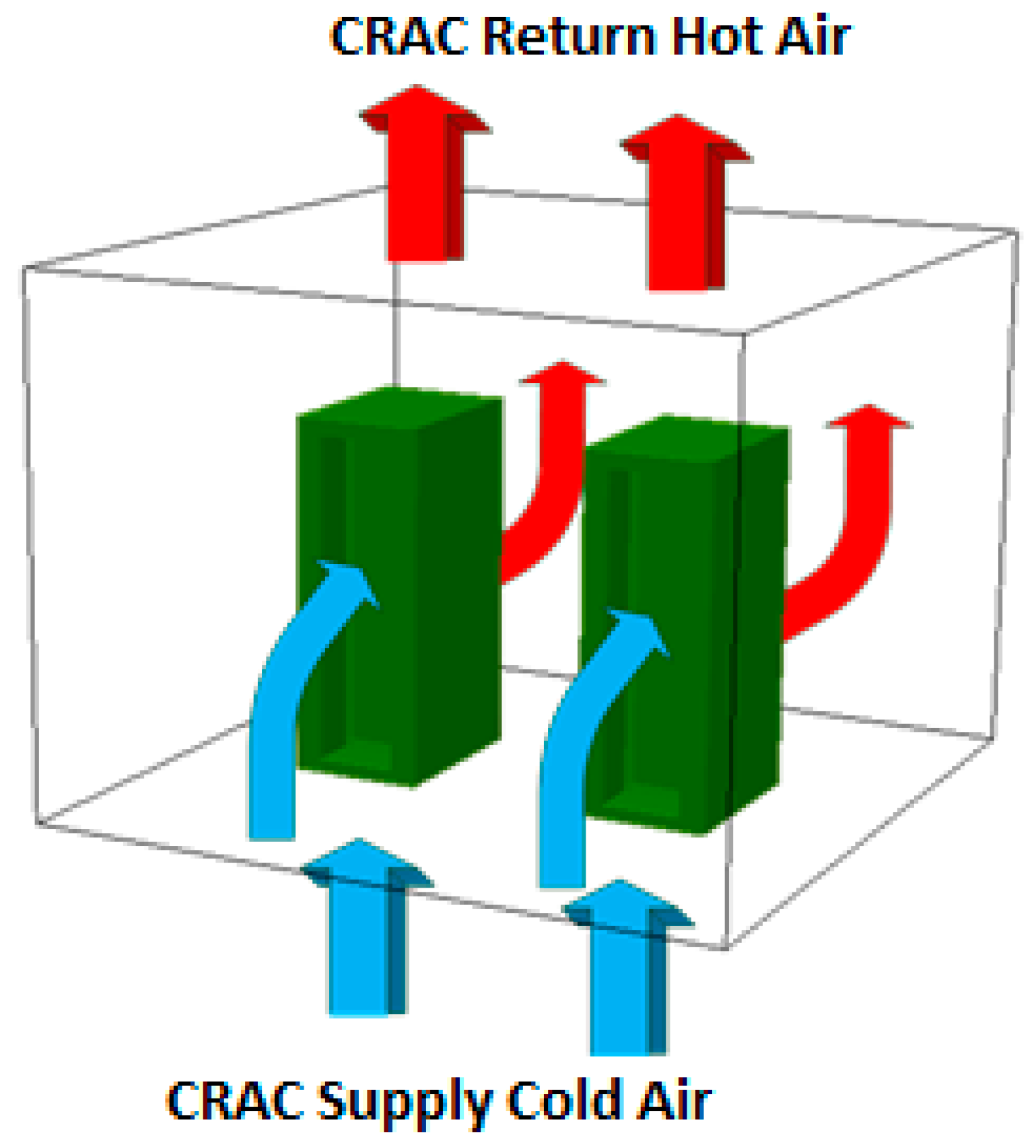
When an air-cooled DC uses heat pumps to dynamically generate thermal energy for heating purposes, the server room is used as a thermal energy buffer that allows increasing or decreasing the heat produced (see Figure 5). This is achieved by modifying the temperature set-points in the server room and deploying and executing more workload on the IT servers to allow thermal energy to accumulate. This will also improve the efficiency of the heat pump operation which operates better at higher temperatures. As it can be seen in relations (1) and (2) minimizing the compressor’s dissipated work $E_{Compressor}$ leads to maximizing both $CO{P}_{Heating}$ and $CO{P}_{Cooling}$ and this happens when the temperature of the air extracted from the server room $T_{HOTAIR}$ is high.

However, increasing the server room temperature set points can lead to potentially disastrous situations, such as equipment overheating and malfunctioning due to hotspot formation in certain areas of the server room. To avoid these risks, before making any decisions a simulation should be performed to validate the new temperature set-points and workload distribution of the IT servers, eliminating the risks of hotspot formation and equipment malfunction. Thermal processes are highly complex and need dedicated simulation tools to achieve accurate and realistic results. The most used methods are based on Computational Fluid Dynamics (CFD) techniques that use numerical simulations to compute the flow of fluids (liquids or gasses) in an area defined by boundary surfaces. Applied in DC thermal distribution simulation, CFD tools report an error of about 1 degree Celsius compared to the real environment, thus being suited for decision analysis regarding server room temperature set-point.

At the same time, CFD-based simulation methods have their own limitations when applied to thermal flexibility studies. Calculations related to a single scenario require a parallel environment and a significant amount of time. Performing CFD for multiple scenarios for every server room in a large-scale DC is costly and time-consuming, being an approach that cannot be considered as affordable and effective in near real time. Thus, to overcome such limitations, in our study we propose to combine CFD simulation with neural networks based methods to predict the temperature distribution in the server room aiming to increase the amount of heat recovered. In this case, the simulations result of numerous configurations of the single simplified setup will constitute the training data set for the neural network based prediction process, which will be used at run time for decision making.

4.2. Server Room Thermal Model

CFD simulations of a virtual server room are used to model the input cold air in terms of pumped airflow and temperature as well as the generated hot air and heat distribution in the server room model for multiple setups. Both the model and the subsequent simulations are prepared with an in-house tool dedicated to the server room CFD analysis, based on the open-source OpenFOAM v4.1 software [32]. To obtain the dynamics of the server room airflow, unsteady Reynolds-averaged Navier-Stokes (URANS) equations together with the two-equational k-ε turbulence model are resolved.

The utilized solver, buoyantBoussinesqPimpleFoam, allows capturing buoyancy effects, taking into account pressure gradient along the vertical dimension, describing static pressure p as:

$$p=p_{rgh}+\rho gh$$

(3)

where: $p_{rgh}$ is the pseudo hydrostatic pressure, $q$ is the air density, $g$ the gravitational acceleration, $h$ the height in the opposite direction to gravity. The solver introduces also the Boussinesq approximation which assumes linear dependency of density and temperature variations. It is applicable to the server room airflow due to relatively slight density fluctuations expected. The approximation reduces nonlinearity and simplifies solved problem. The effective density $q_k$, present in the gravity term of momentum equation, is expressed with the following equation:

$${\rho }_k=1-\beta \left(T-T_{ref}\right)$$

(4)

where $\beta$ is the thermal expansion coefficient, $T$ the temperature, $T_{ref}$ the reference temperature. Such an approach makes the solver incompressible. The solver uses the PIMPLE pressure-velocity coupling algorithm to obtain a transient solution, which is a combination of Pressure Implicit with Splitting of Operator (PISO) and Semi-Implicit Method for Pressure-Linked Equations (SIMPLE) schemes.

The server room is modelled considering its size (width × depth × height) as well as the racks deployed in it. In general, the utilized CFD tool allows modelling a rack both as a set of separate servers of any occupation pattern or as a simplified single device. Due to performance reasons, we chose the second approach. The racks are considered as fully and homogeneously occupied with servers, their geometry is simplified in a way that each of the racks is treated as single airflow and heat source. They are provided with one inlet and one outlet each, allowing the use of less computationally expensive mesh. Cold air is supplied into the room through the floor surface whereas the return air stream leaves through the ceiling. The intention of such Computer Room Air Conditioning (CRAC) modelling was to create a possibly generic case, independent from location and number of floor supply tiles and return outlets. The virtual server room model used in this study is presented in Figure 6.

To properly model each rack as heat sources and to keep the power of racks at a constant level during every simulation execution, swak4Foam [33] library (Swiss Army Knife for Foam) was utilized. It allows binding boundary conditions with functional dependency of one from another with groovyBC utility. While at racks inlets the temperature was forming freely, at racks’ outlets, on the other hand, the temperature boundary condition was characterized as a function of inlet temperature, to fulfil below heat balance equation:

$${\rho }_k=1-\beta \left(T-T_{ref}\right)$$

(5)

where $P_r$ is the heat output of rack, ${\rho }_{ref}$ is the reference density (1.1884 kg/m³ for reference $p_{rgh}$ = 100 kPa and $T_{ref}$ = 20 °C), $Q_r$ is the rack airflow volume (2.0 m³/s, ≈0.048 m³/s per U), $C_p$ is the specific heat capacity (1003.98 J/kgK), $T_{HOTAIR}$ is the rack outlet temperature and finally $T_{COLDAIR}$ is the rack inlet temperature. For this study, it is assumed, that 100% of racks power consumption is responsible for heat generation. The final form of the outlet temperature equation is stated below:

$$T_{HOTAIR}=T_{COLDAIR}+\frac{P_r}{{\rho }_{ref}{Q}_r{C}_p}$$

(6)

4.3. Predicting the Heat Distribution

The CFD experiments described above compute the temperature of the hot air generated in the server room ($T_{HOTAIR}$) considering $M$ virtual probes, the simulation outputs $T_{HOTAIR}^{Probe\left[m\right]}[t]$ where $m\in \{1\dots M\}$ and $t$ is the time instance when the data was taken (see Figure 7). The probes are deployed at the inlet and outlet of the $K$ racks as well as at the outlet of the server room. The simulation input is defined by the initial room temperature ($T_{ROOM-INITIAL}$), the temperature of the air pumped by the cooling system in the server room ($T_{COLDAIR}$) and its flow ($ai{r}_{FLOW}$) and the heat generation of the $K$ racks modelled ($Hea{t}_{Rack}[k],k\in \{1\dots K\}$).

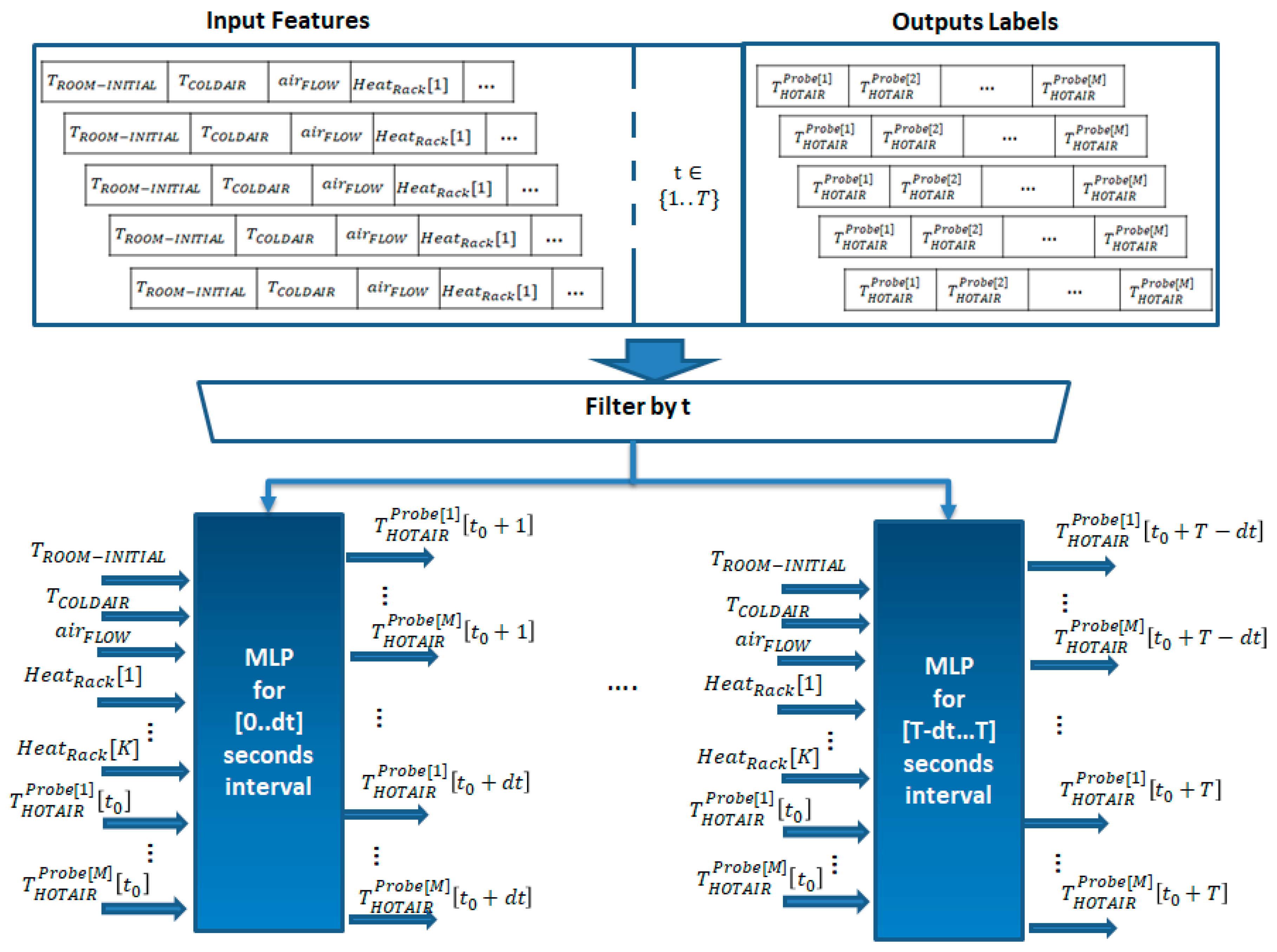
The CFD input parameters are varied to generate $N$ different scenarios, each run over an interval of $T$ seconds to compute the temperatures for the $M$ probes. The generated data are fed to a neural network based infrastructure with the goal of predicting the heat distribution in the server room and the temperature of the hot air generated. The forecasting infrastructure is based on neural networks of type Multi-Layer Perceptron (MLP) featuring 4 fully-connected layers of neurons of type ReLU (Rectified Linear Units). The input layer has $K+3+M$ neurons, the other two hidden layers have $\alpha (K+3+M)+\beta$ neurons, while the output layer has $dt\times M$ neurons, where $dt$ is the number of seconds for which each MLP will predict the probe temperatures.

Because we need predictions for every second in the $[0\dots T]$ forecasting interval, the developed infrastructure has $M_T=\frac{T}{dt}$ MLP modules trained with data filtered for a specific second ($t$ in Figure 7) to compute temperature predictions of the $M$ probes for that time instance. Each of the T MLPs has as input the $K+3$ parameters ($T_{ROOM-INITIAL}$, $T_{COLDAIR}$, $ai{r}_{FLOW}$, {$Hea{t}_{Rack}[i],i\in \{1\dots K\}$}) describing the initial situation of the simulation and additional $M$ parameters describing the temperature probe values at the beginning of the prediction window $T_{HOTAIR}^{Probe[m]}[t_0]$. Each MLP module aims at predicting the temperature of the $M$ key points representing the probes deployed in the server room for every timestamp $t$ in each time interval of the form $ML{P}_{domain}(i)=[i\times dt,(i+1)\times dt],$ where $i\in \{0\dots M_T-1\}$. Thus, for computing the all the hot air probe temperatures at second t in the future, the index $i$ of the interval $ML{P}_{domain}(i)$ has to be computed as the integer part of the ratio $i=[\frac{t}{dt}]$, and the temperatures will be predicted by the $ith$ MLP as its $\left(t-i\times dt\right)$ outputs:

$$T_{HOTAIR}^{Probe\left[m\right]}\left(t_0+T\right)=ML{P}_i\left(T_{ROOM-INITIAL},T_{COLDAIR},ai{r}_{FLOW},Hea{t}_{Rack}\left[K\right],T_{HOTAIR}^{Probe\left[M\right]}\left[t_0\right]\right)\left[t-i\times dt\right]$$

(7)

For looking forward into the future and predicting the server temperature at deployed probes over periods larger than the CFD simulations of $T$ seconds, we proposed the iterative algorithm shown below (Algorithm 1). The algorithm inputs are the initial parameters of a simulation and the time for which the prediction has to be computed, while the outputs are the M simulation output parameters after the simulation time $Tim{e}_{prediction}$.

Algorithm 1. Heat Prediction Algorithm for Long Time Periods

Input:$T_{ROOM-INITIAL},T_{COLDAIR},ai{r}_{FLOW},Hea{t}_{Rack}\left[k\right],Tim{e}_{prediction}$

Output:$T_{HOTAIR}^{Probe\left[m\right]}\left[Tim{e}_{prediction}\right],m\in M$

Begin

$Interval{s}_T=\frac{Tim{e}_{prediction}}{T}$// iterate over the interval$\left[0\dots Tim{e}_{prediction}\right]$with time step of length$T$

$Inde{x}_T=Tim{e}_{prediction}\%T$// compute time interval remaining that cannot be covered by time steps of length$T$

$I_{MLP}^{iterations}=\frac{T}{dt}$// compute MLP index within T interval

$Outpu{t}_{MLP}^{iterations}=T\%dt$// compute output index within the MLP

$I_{MLP}^{final}=\frac{Inde{x}_T}{dt}$//compute MLP index within last$Inde{x}_T$interval

$Outpu{t}_{MLP}^{final}=Inde{x}_T\%dt$//compute output index within last MLP

$t_0=0$

$\mathrm{For}\left(time=1toInterval{s}_T\right)$ Do

For $\left(m=1toM\right)$ Do

$T_{HOTAIR}^{Probe\left[m\right]}\left[t_0+T\right]=ML{P}_{I_{MLP}^{iterations}}\left(T_{ROOM-INITIAL},T_{COLDAIR},ai{r}_{FLOW},Hea{t}_{Rack}\left[K\right],T_{HOTAIR}^{Probe\left[m\right]}\left[t_0\right]\right)\left[Outpu{t}_{MLP}^{iterations}\right]$

$t_0=t_0+T$; $m=m+1$

End For

$T_{HOTAIR}^{Probe\left[1\dots M\right]}\left[Tim{e}_{prediction}\right]=ML{P}_{I_{MLP}^{final}}\left(\begin{array}{c}{T}_{ROOM-INITIAL},T_{COLDAIR},ai{r}_{FLOW},Hea{t}_{Rack}\left[K\right],\\ T_{HOTAIR}^{Probe\left[M\right]}\left[Interval{s}_T\times T\right]\end{array}\right)\left[Outpu{t}_{MLP}^{final}\right]$

Return $T_{HOTAIR}^{Probe\left[1\dots M\right]}\left[Tim{e}_{prediction}\right]$

End

The algorithm starts by computing the number of $T$ second intervals included in the prediction period $Tim{e}_{prediction}$. Furthermore, it computes the index of the MLP used to predict T seconds in the future, and the index of the output of the MLP corresponding to this prediction. It also computes the length of the last interval that cannot be covered by intervals of length T, the index of the MLP and the index of the MLPs output to compute the last prediction. Then, it performs iterations over these intervals and for each interval it computes the average room temperature in the M probes, while updating the time for the next prediction. Finally, it calls the MLP for the last time interval of length $I_{MLP}^{final}$ to compute the final values of the probes.

5. Evaluation Results

We had used the proposed DC heat reuse model to investigate the thermal energy flexibility potential of a virtual server room from PSNC DC modeled with CFD aiming to predict the temperature of the air inside which can be recovered using a heat pump and delivered to nearby neighborhoods. The virtual server room modeled with CFD has the size of 4 m × 4 m × 3 m (width × depth × height) and is equipped with two typical 42U racks (0.8 m × 1.07 m × 2.05 m respectively). They are provided with one inlet and one outlet (width: 0.45 m, height: 42U ≈ 1.8669 m), allowing the use of less computationally expensive mesh. Figure 8 reflects the virtual server room in OpenFoam environment. It was assumed, that between all the scenarios, five key parameters are changed, according to

Table 1. List of parameters variation for simulation scenarios.

Parameter	Min	Max	Step
Initial room temperature: $T_{INITIAL-ROOM}$ [°C]	18	26	2
Air conditioning volume flow rate: $ai{r}_{FLOW}$ [m3/s]	0.6	1.8	0.3
Air conditioning outlet temperature: $T_{COLDAIR}$ [°C]	10	18	2
Power consumption of rack no 1: $P_1\left[\mathrm{kW}\right]\cong HEA{T}_{Rack-1}$	2	10	2
Power consumption of rack no 2: $P_2\left[\mathrm{kW}\right]\cong HEA{T}_{Rack-2}$	2	10	2

.

From all received results, the temperature values at specific locations were extracted for every 1-s time interval of total 600-s (10 min) time range of every run. Virtual temperature probes were located at I/O surfaces in the domain, except CRAC supply outlet, where the temperature was fixed during the execution. List of probes together with their count and location is placed in

Table 2. List of temperature probes in virtual server room.

Probed I/O Surface	Probe Count	Probe Location
CRAC return duct inlet	4	(1,1,3), (1,3,3), (3,1,3), (3,3,3)
Racks outlets	1 (× 2)	1.025 m above floor surface (half of the rack height, at outlet vertical symmetry axis)
Racks inlets	4 (× 2)	0.465 m, 0.838 m, 1.212 m, 1.585 m above floor surface (evenly spaced along vertical inlet dimension, at inlet vertical symmetry axis)

.

All possible CFD-based simulations (considering the Table 1 parameters) were executed and this generated over 200 GB of output data, from which probe data were extracted. Taking into account the number of probes $N_p=14$ and the number of collected time steps per execution $N_t=600$, the total number of temperature records per simulation is equal $N_{ts}=N_p\times N_t=8400$ and the sum for whole described study $N_{tt}=N\times N_p\times N_t\approx 26M$. 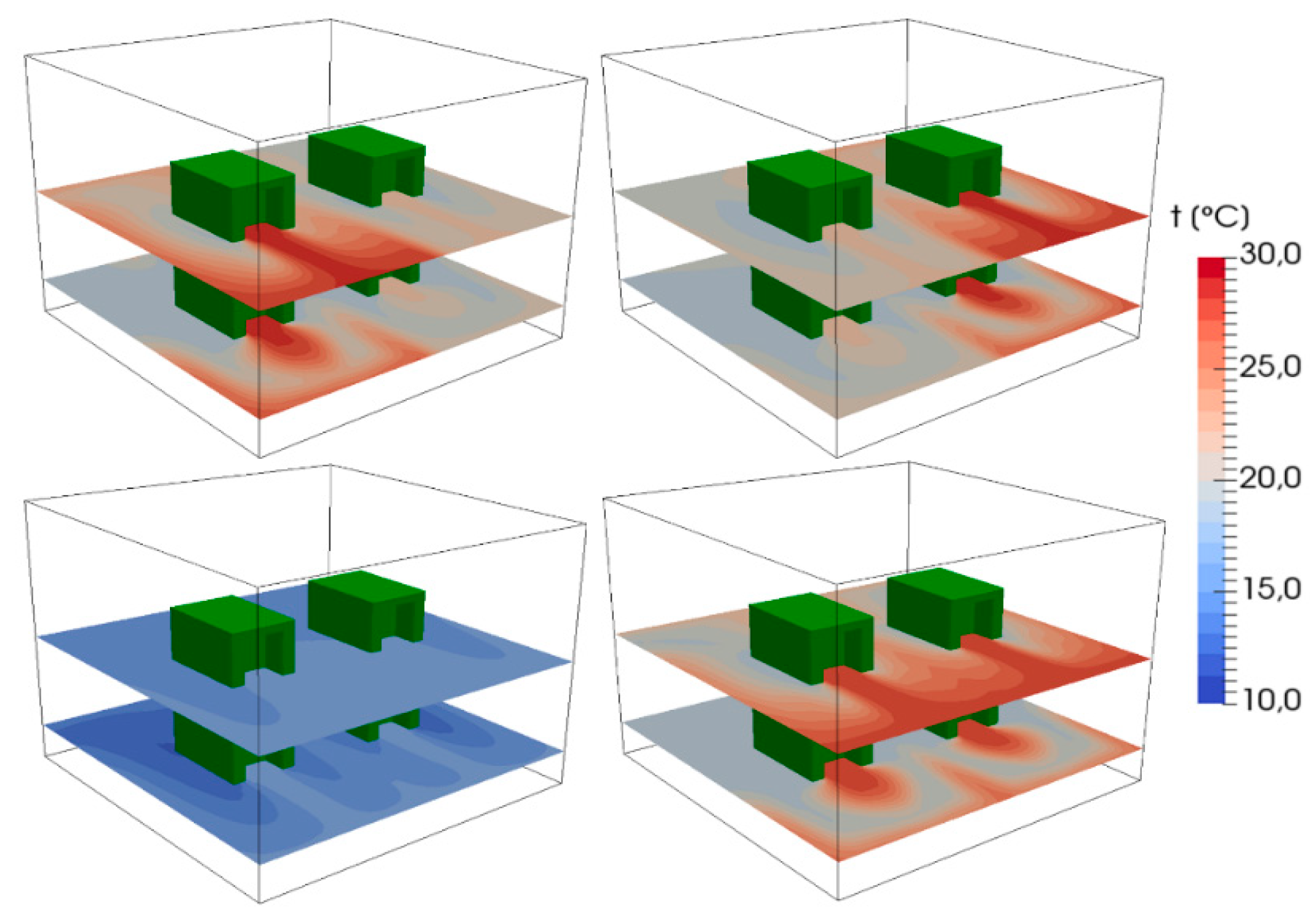The generated data will constitute the training data of our prediction algorithm. Exemplary results for different air conditioning volume flow rate can be seen in Figure 9.

We had varied the five input parameters of the CFD simulation defined in Table 1 to generate 3125 different scenarios, each scenario being run over a period of 600 s to compute the temperatures for the 14 probes defined in

Table 3. MSE of simulation outputs for the tested scenarios.

Output	Average MSE
$Rac{k}_{inlet-1}^1$	0.028
$Rac{k}_{inlet-2}^1$	0.029
$Rac{k}_{inlet-3}^1$	0.034
$Rac{k}_{inlet-4}^1$	0.046
$Rac{k}_{outlet}^1$	0.019
$Rac{k}_{inlet-1}^2$	0.025
$Rac{k}_{inlet-2}^2$	0.036
$Rac{k}_{inlet-3}^2$	0.040
$Rac{k}_{inlet-4}^2$	0.041
$Rac{k}_{outlet}^2$	0.035
$Roo{m}_{outlet}^1$	0.091
$Roo{m}_{outlet}^2$	0.087
$Roo{m}_{outlet}^3$	0.032
$Roo{m}_{outlet}^4$	0.038

at each second thus generating 8400 output values. Thus we had chosen to split the main dataset into 60 sub-datasets, each used to train the neural networks based algorithm to predict the 14 outputs of the simulation for every second of a 10 s time interval within the 600 s prediction interval. In total, we create 60 datasets for each scenario, that will be used to train 60 MLPs. Thus, for each second within each 10 s simulation interval we created 3125 training pairs, associating the parameters of each simulation with the output to be predicted at a given timestamp in the future. We train the MLP-based prediction infrastructure defined by splitting the data set in 90% training data and 10% test data.

The first evaluation aims at determining the temperature prediction performance over the test scenarios. For each scenario, the Mean Square Error (MSE) was computed for each predicted output defined in Table 3 over the 600 s simulation interval and it was compared against the reference CFD scenario:

$$MSE\left(output\right)=\frac{1}{312}\times {\displaystyle \sum _{i=1}^{312}}\frac{1}{600}({\displaystyle \sum _{t=1}^{600}}(output\left(t\right)-ML{P}_{\frac{i}{60}}\left[i\%10\right]))$$

(8)

As it can be seen from the table above, the predictions exhibit an error of less than 0.1 that corresponds to less than 1 degree Celsius, being suited for real time temperature evaluation to avoid hot spots.

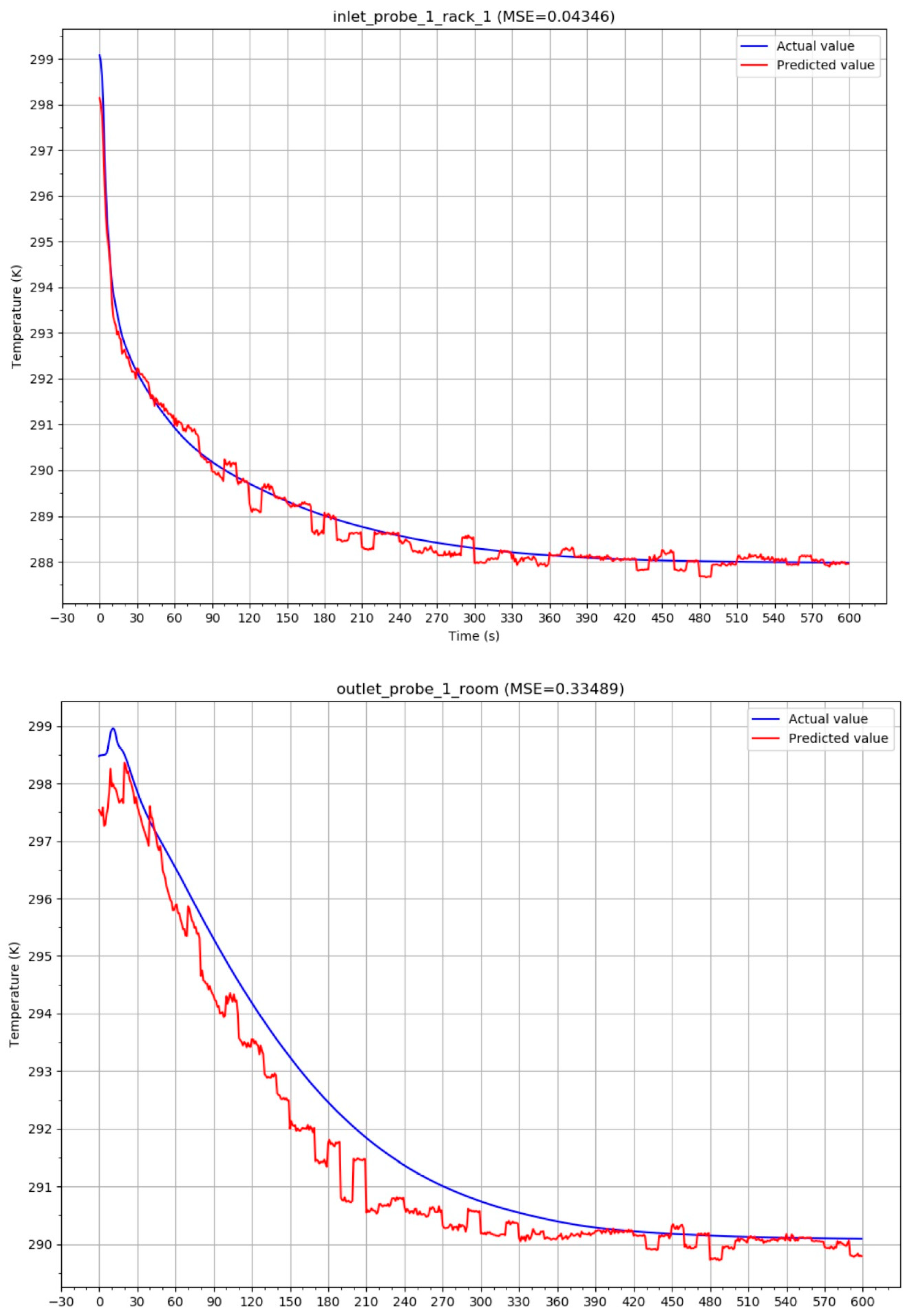
The temperature evolution prediction compared with the one generated by the CFD can be seen in Figure 10 for one of the scenarios run. The red lines represent the predicted values while the blue lines represent the real temperature values taken from the simulation. It can be seen for the sample probes even for the worst MSE the predicted temperature profile follows closely the real temperature profile, exhibiting errors of roughly 1 degree Celsius.

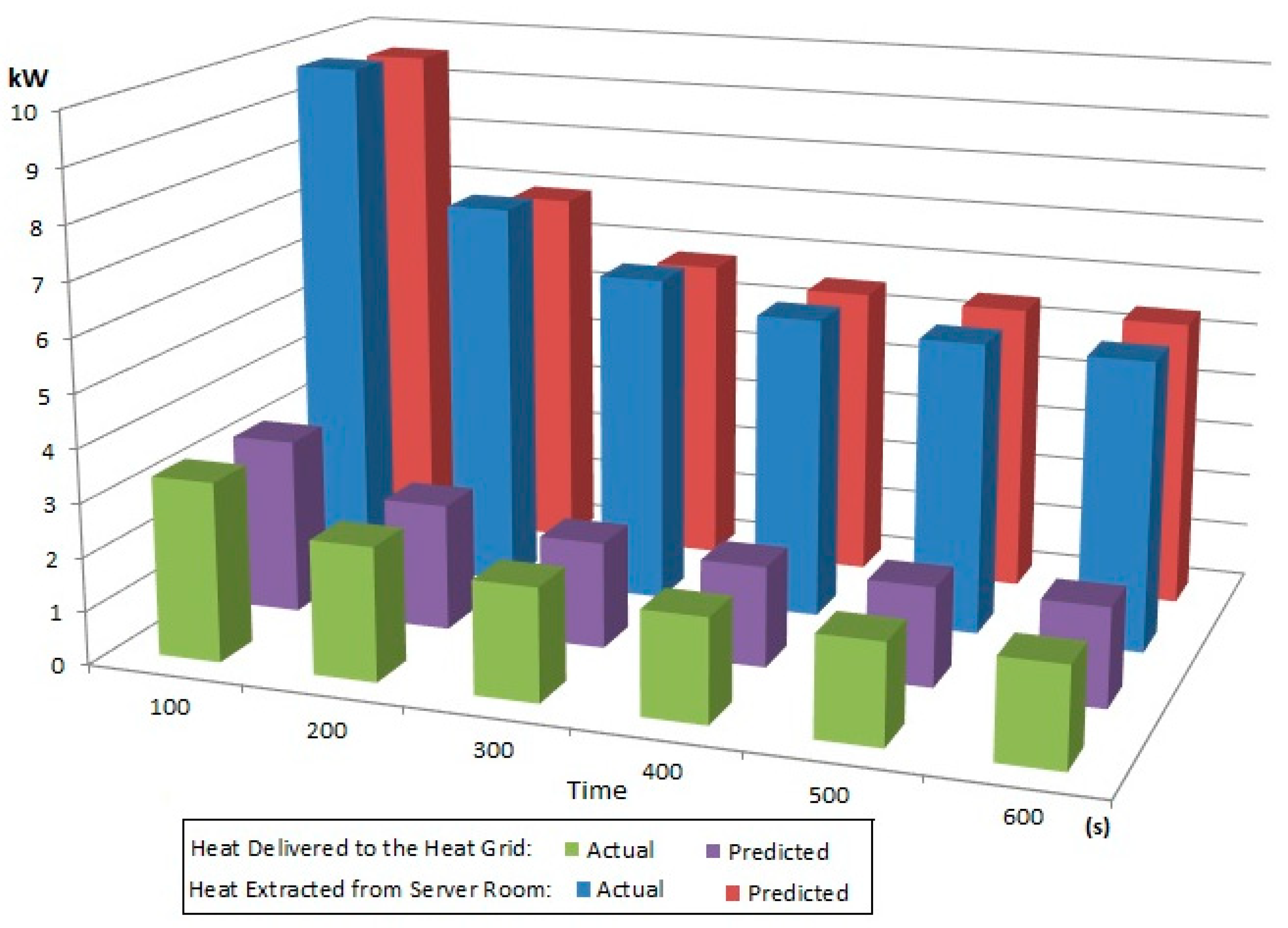
Figure 11 show the impact of prediction errors onto amount of waste heat estimated to be delivered to the heat grid in comparison with the actual ones. We have considered a heat pump featuring a $CO{P}_{Cooling}=3.8$ and a $CO{P}_{Heating}=2.3$ and the hot air temperatures in the server room reported in Figure 10 (BOTTOM). As it can be seen the impact is almost negligible showing that our solution could be successfully used by DC managers to accurately estimate the amount of available heat to be injected at future time frames. At the same time, the correlation between the amount of heat actually recovered from the server room the one delivered and indirectly with the temperature of the hot $T_{HOTAIR}$ at server room outlet can be clearly seen. The higher the temperature of the hot air extracted is the higher the temperature of the heat delivered to the heat grid (assuming a constant energy consumption of the heat pump compressor) is too.

In terms of the economics of heat reuse with respect to the requirements and example presented in Section 3.1, we have estimated the potential cost and savings related to the installation of the heat transfer system. The calculation was made on the following assumptions: (i) DC generated heat for winter period (based on data presented in Figure 1, linear estimation of winter period heat production is 7400 GJ annually) is much higher than total heat demand of PSNC buildings A and B (annual heat demand, based on the metered average value is less than 7000 GJ) and (ii) the DC waste heat is transferred to buildings A and B. Waste heat could be potentially be reused in building C, but detailed calculations of heat cost produced by heat pumps in the building will be conducted within a year, based on real exploitation, and then the final decision will be made. As the current design of buildings B-C water loop assumes only 250 kW power the pipes diameters should be increased to obtain higher power, about 1.75 MW.

District heating heat cost in PSNC, Poland is 20 €/GJ which gives 125,460 € annually since the yearly heating demand is 6273 GJ. There are three options of the heat consumption from district heating providers. In the first option the heat is still delivered by a district heating operator. For the second option, even if no energy is consumed from a district heating, maintaining the current levels of contracted power demand values, gives the annual heating station costs of 52,750 €. In the third option the contracted power demand is left on the same level as in present but only for a short period of time to make sure the system works properly. As the certainty of heat supply is important for PUT, this is the best option. Renouncing at the heating stations in the third option will reset the annual heating cost from the district heating to 0 €. The price of the heat from PSNC was assumed at 2 €/GJ and the cost of energy appliances (pumps, heat pumps) as well as maintenance costs at the level of 11,628 € annually. These are examples of values based on the assumption that the investment in the required infrastructure is done by PUT (hence even low PSNC heat price is profitable). In the next steps, other options will be considered, including separate ROI estimations for both PSNC DC and the PUT campus. A cost summary of these three options is presented in

Table 4. Operational costs analysis for the three heat reuse options considered.

Annual Cost Components	Option 1 Contracted Power Demand 1.527 MW, DH Heat Demand 6273 GJ/year	Option 2 Contracted Power Demand 1.527 MW, DH Heat Demand 0 GJ/year	Option 3 Contracted Power Demand 0 MW, DH Heat Demand 0 GJ/year
A+B buildings district heating cost	125,460 €	52,750 €	0 €
PSNC DC heat revenues (6273 GJ annually, 2€/GJ)	N/A	12,546 €	12,546 €
Water loop running cost (pumps—electricity, maintenance)	N/A	11,628 €	11,628 €
Savings	N/A	48,536 €	101,286 €

.

In the consideration of capital expenditures, we assume that the investment in the required infrastructure is done by PUT. Water loop cost with heat pumps and pumping stations estimation is 1,150,000 €. Operational cost estimation was based on current district heating and electricity cost, whereas capital cost was based on real expenditures of the ongoing building C investment process. For Option 2 presented above (and in Table 4) with annual savings of 101,286 €, Simple Pay Back Time (SPBT) is 11.4 years, while Net Present Value (NPV) with 3% discount rate is 59,000 € in 15 years’ period. With 50% EU investment subsidy SPBT would be 5.7 years while NPV 56,000 € in 7 years’ period. Without subsidies and with district heating contracted power demand of 1.527 MW assurance (option 2 above) the installation of the heat transfer system is unreasonable due to SPBT of 23.7 years. Summary of these values is presented in

Table 5. Capital expenditures analysis results for the three heat reuse options considered.

Option	SPBT	NPV (3% Rate)
No subsidies, DH contracted power demand 1.527 MW—Option 2 -	23.7 years	N/A
No subsidies, No DH connection (contracted power demand 0 MW)—Option 3 -	11.4 years	59,000 € (15 years)
50% subsidies, No DH connection (contracted power demand 0 MW)—Option 3 -	5.7 years	56,000 € (7 years)

below. The potential use of existing pipes network of Poznan district heating could significantly reduce project costs and will be further investigated during future works.

6. Conclusions

In this paper, we have defined models and techniques for predicting the temperature of the air inside a server room which can be recovered and transferred by means of heat pumps to nearby neighborhoods. We proposed CFD simulations to evaluate a large number of scenarios which impact the temperature of the air. We defined a neural network-based prediction method which takes as input a large amount of data generated by means of CFD simulations to forecast the server room temperature overcoming the simulations’ time and computational overhead at run time. The prediction process showed good performance having an error rate of less than 1% in predicting the server room temperature which represents less the 1 degree Celsius.

For the next steps, we plan to extend our work to the entire Poznan Supercomputing and Networking Center. This is in line with the current objectives of the collaboration between PSNC and Poznan University of Technology to perform a feasibility study of the heat transfer system between the PSNC DC to the PUT facilities. For now, we analyzed the current heat demands of PUT facilities, described existing infrastructure and showed corresponding economic analysis. The analysis has shown high potential. The return on investment time was initially estimated as 5.7–11.4 years depending on concrete heat demand/supply and price of heat defined by PSNC. However, current PSNC heat production is not sufficient to cover the worst-case demand (around 1.5 MW when the temperature falls to −18 °C) even if it fits the typical demands (0.5–0.75 MW for temperatures within 0–8 °C). For this reason, an approach with a connection to the heating network will be also considered, and accurate prediction and control of thermal flexibility presented in this paper is needed to achieve high efficiency and reliability.