Increasing the Utilization of Transmission Lines Capacity by Quasi-Dynamic Thermal Ratings


1
School of Mechanical, Electrical and Information Engineering, Shandong University (Weihai), Weihai 264209, China
2
Department of Mechanical-Electrical Engineering, Weihai Vocational College, Weihai 264210, China
3
State Grid Weihai Power Supply Company, Weihai 264200, China
*
Author to whom correspondence should be addressed.
Energies 2019, 12(5), 792; https://doi.org/10.3390/en12050792
Submission received: 23 January 2019
/
Revised: 17 February 2019
/
Accepted: 25 February 2019
/
Published: 27 February 2019
Abstract
:The power grid is under pressure to maintain a reliable supply because of constrained budgets and environmental policies. In order to effectively make use of existing transmission lines, it is important to accurately evaluate the line capacity. Dynamic thermal rating (DTR) offers a way to increase the utilization of capacity under real-time meteorological data. However, DTR relies on a number of sensors and the cost is high. Therefore, a method of improving the utilization of capacity by quasi-dynamic thermal rating (QDR) is proposed in this paper. QDR at different confidence levels and time scales is determined through the statistical analysis of line ampacity driven by key parameters, and the key parameters is identified by control variate method. In addition, the operation risk and tension loss is evaluated. The results show that QDR can increase the utilization of line capacity and in the absence of along-line measuring devices, QDR is more accurate, reliable and cost-saving. The managers can determine the appropriate confidence level according to the operation risk and tension loss that the system can bear, and shorten the time scale with the permission of the operation and control complexity.
1. Introduction
In view of the challenges of new energy generation, load growth and obsolete distribution facilities, it is imperative to improve the utilization of transmission line capacity [1]. However, due to the scarcity of space and land, there is great difficulty in building new transmission corridors [2]. Therefore, it is particularly important to accurately evaluate the maximum allowable ampacity and tap the transmission potential of existing lines to make full use of power grid resources [3].
The transmission capacity is limited by thermal load, so the research on the thermal load capability of transmission lines is of great significance [4]. The traditional static thermal rating (STR) uses severe meteorological conditions to determine the maximum allowable ampacity of the line [5], whose result tends to be conservative and reduces the utilization of the line. With the rapid development of sensor technology, the meteorological data obtained by the meteorological measurement devices are used to determine the real-time capacity [6]. Therefore, dynamic thermal rating (DTR) has gradually become a research hotspot [7]. Subsequently, meteorological numerical prediction technology has gradually gained widespread attention. In [8], the meteorological prediction technology applied to DTR is introduced. Compared with STR, DTR makes full use of the hidden capacity of transmission lines under the safe operation of the power grid, and the utilization of capacity is greatly increased [9]. However, the high cost of the monitoring equipment makes it difficult to implement [10]. Moreover, due to the randomness of meteorological data, there are some errors between the data obtained from the meteorological numerical prediction devices and real-time data, which often leads to the calculation results of DTR deviate from the actual operation [11]. In addition, the time variant of DTR increases the complexity of system operation and control [12]. Therefore, the concept of quasi-dynamic thermal rating (QDR) was proposed in [13]. QDR is constant in a certain time scale. Compared with DTR, although QDR is slightly conservative, it is more reliable and less costly to implement [14]. In [15], the historical data of key meteorological parameters were analyzed statistically to determine their thresholds in different confidence levels and time scales, and then the QDR in corresponding time scales were calculated by using the thresholds. However, the thresholds at the same confidence level cannot occur simultaneously, so the method is conservative. Therefore, based on the change of key meteorological parameters, a method for determining QDR of long time scale by statistical analysis of line ampacity is proposed in this paper. The results show that QDR can effectively improve the utilization of the line capacity. The conclusion can provide a basis for decision-making of line thermal rating method in power sector, and give some important suggestions for the selection of time scale and confidence level.
The rest of this paper is organized as follows: in Section 2, the heat balance equation based on CIGRE (International Council on Large Electric systems) standard, the concept of QDR, and the assessment method of operation risk and tension loss are introduced. In Section 3, based on the heat balance equation, control variate method is used to analyze the influence degree of conductor parameters and meteorological parameters on ampacity and identify the key parameters. The necessity of dividing time scales (year, season, month) is illustrated by statistical analysis of historical data of key parameters in Section 4. In Section 5, based on the historical key data in corresponding time scales, the maximum allowable ampacity is calculated, and the QDR under different confidence levels is determined by statistically analysis of the ampacity. The operating annual meteorological data is used to evaluate operation risk and tension loss of QDR. Discussion and conclusions are given in Section 6 and Section 7, respectively.
2. QDR and Operation Risk Assessment of Transmission Line
2.1. Heat Balance Equation
The conductor temperature depends on the heat generated by the current passing through the line and absorbed from solar radiation, the convection heat generated by wind, and the radiation heat due to the temperature difference between the conductor and ambient temperature. At present, CIGRE [16] and IEEE standard [17] are two representative methods to characterize the relationship between conductor temperature and ampacity. It is assumed that the transmission line is a uniform conductor. According to the CIGRE standard, neglecting the influence of small quantity on the heat balance equation, such as evaporation heat loss and corona loss, the heat balance equation is shown in Equation (1):
where qc is the convection heat, related to ambient temperature, wind speed, wind direction, conductor surface condition and aggregation state, which is the main way of conductor heat dissipation; is the radiation heat related to conductor temperature, ambient temperature, conductor diameter and surface emissivity; is the absorption heat from solar radiation, which is not only related to the intensity of the sunshine and the height of the sun, but also related to the conductor diameter and surface absorptivity; is the conductor resistance at the temperature of ; is the ampacity. The detailed expressions of above parameters are shown in [18]. The ampacity made the conductor temperature reach the maximum allowable value can be obtained by Equation (2):
qc + qr = qs + I2R(Tc)
2.2. Quasi-dynamic Thermal Rating
STR is static, set according to the worst weather conditions. Because the worst weather conditions are rare, this method is conservative and therefore, it wastes available capacity. In order to increase the utilization of available capacity, QDR changes the time scale (yearly, seasonally, monthly) to take advantage of different weather conditions during different parts of the year. According to different time scales, all historical meteorological data are divided into different subsets. The maximum allowable ampacity is calculated using the data from each subset. QDR under different confidence levels is determined by statistical analysis. For example, calculate QDR at 99% confidence level in December based on eight-year historical meteorological data. Firstly, all the meteorological data in December of eight years are grouped into a subset. Next, the maximum allowable ampacity is calculated using the subset. Finally, the QDR at 99% confidence level in December is determined by statistical analysis of the ampacity, which means 99% of the ampacity are greater than QDR. represents the QDR under the confidence level and the th time scale , which satisfies the following constraints shown in Equation (3):
where is the sample number that the ampacity greater than QDR under the year and the time scale . is the number of the statistical years. is the sample number of the ampacity under the year and the time scale . is the number of time scales divided in one year. If the time scale is year, ; if the time scale is season, ; if month, . is the total number of samples in all the statistical years.
2.3. Operation Risk and Tension Loss Assessment
Assuming that is the collection of meteorological data such as wind speed, wind direction and ambient temperature at a certain time. The QDR of transmission lines under self-limiting and ambient environment can be calculated by Equations (2) and (3). When the current flowing through the line is QDR calculated, the actual operating temperature of the conductor under is obtained by the heat balance equation, and the frequency of is shown in Equation (4):
where is frequency of .
The probability of conductor temperature exceeding is calculated by the frequency of , which is the operation risk corresponding the QDR, as shown in Equation (5):
If the temperature of an aluminum conductor is greater than 95 °C, the high conductor temperature will cause conductor tension loss. In [19], the percent loss of tensile strength of an aluminum conductor strand can be determined as Equation (6):
where is the temperature of conductors, and t is the exposure time in hours. The total loss of tensile strength in a composite conductor can be computed as Equations (7)–(9):
where r is the strand diameter, n is the number of strands and S is the strand strength for the individual components (e.g., aluminum Al, and steel St). According to Equations (6)–(9), considering the allowable limit of 15% loss of tensile strength, the life expectancy of the strands is 51 years at 110 °C, but it is about 3 months at 120 °C, and only 78 h at 140 °C, 23 h at 150 °C.
3. Identification of Key Parameters
There are two main factors affecting the ampacity of lines. One is the conductor parameters, including conductor diameter, maximum allowable operating temperature, solar absorptivity, emissivity and so on; the other is the surrounding meteorological parameters, including wind speed, wind direction, ambient temperature, sunshine intensity, solar hour angle, sun declination angle and so on. The meteorological data with the interval of one hour are from the Observatory of Shandong University in Weihai, China, from 1 January 2015 to 31 December 2015. It is of great significance to identify the key parameters affecting the ampacity. In this section, the key parameters affecting the ampacity are identified by the method of control variate, that is, one input parameter is varied while the other inputs are fixed [20]. The influence degree is based on the ampacity difference caused by a variable parameter. The conductor parameters and meteorological parameters are as follows.
The type of transmission line in this paper is LGJ-400/50, whose diameter is 27.63 mm and the maximum allowable operating temperature is 70 °C. For the emissivity and solar absorptivity, few values are selected, such as 0.23, 0.5, 0.7 and 0.9. For new conductors, the values of emissivity and absorptivity can be as low as 0.23 and for old conductors, these can be up to 0.9 [21]. Considering the conductor is moderately old, both absorptivity and emissivity are taken as typical value of 0.5 in this paper. In addition, ranges of wind speed, wind incidence angle, and ambient temperature corresponds to the ranges of real conditions from 1 January 2015 to 31 December 2015 and the fixed values are selected as the average. The ranges of sunshine intensity and declination angle are taken as the maximum and minimum of theoretical values calculated by CIGRE standard. The fixed value of sunshine intensity is taken as 0 W/m2 in night and the average in day. The fixed value of declination angle is taken as 0°. It is stipulated that the solar hour angle at noon is 0° taken as the fixed value, which varies at 15° per hour, negative in the morning and positive in the afternoon. The fixed values and ranges of above parameters are listed below:
- emissivity: 0.5 (0.23, 0.5, 0.7, 0.9)
- solar absorptivity: 0.5 (0.23, 0.5, 0.7, 0.9)
- wind speed: 6.2 (0–20.4 m/s)
- wind incidence angle: 45° (0°–90°)
- ambient temperature: 14.0°C (−8.1 °C–38.2 °C)
- sunshine intensity: 668 W/m2 (0–1335.7 W/m2)
- declination angle: 0° (−23°39’–23°39’)
- solar hour angle: 0° (−180°–180°)
The ampacity difference caused by single parameter variation is shown in Table 1. The meteorological parameters including wind speed, ambient temperature and wind incidence angle have great influence on ampacity, followed by emissivity and sunshine intensity, while solar hour angle, solar absorptivity and declination angle have little influence on ampacity.
4. Statistical Analysis of Key Meteorological Parameters
The meteorological data used in this section include wind speed, wind direction and ambient temperature in 10 min interval from 1 June 2009 to 21 May 2017 in Observatory of Shandong University in Weihai, China. The statistics of the key meteorological parameters in the past eight years are as follows.
4.1. Wind Speed
The maximum wind speed is 22.7 m/s. The maximum difference of the maximum frequency wind speed in different years is 0.8 m/s. Similarly, the wind speed difference of the same season in different years is 6.9 m/s, and the difference of the same month in different years is 7.4 m/s. The above differences illustrate that it is necessary to use historical statistics of meteorological parameters to drive the thermal rating of the line.
In the same years, the maximum differences of the maximum frequency wind speed in different seasons and months are 6.1 m/s. The differences indicate the necessity of dividing time scale of thermal rating. The frequency distribution histogram of the eight-year wind speeds is shown in Figure 1.
4.2. Ambient Temperature
According to statistics, the maximum and minimum temperatures are 42.0 °C and −13.5 °C, respectively. The maximum annual temperature difference is 51.9 °C. The maximum difference of the average temperatures in different years is 2.0 °C. Similarly, the maximum differences of the same seasons and the same months in different years are 4.7 °C and 6.3 °C respectively. In the same year, the maximum differences of the average temperatures in different seasons and months are 24.5 °C and 29.0 °C, respectively. The above temperature differences show the necessity of QDR in different time scales based on meteorological data. The frequency distribution histogram of the eight-year ambient temperatures is shown in Figure 2.
4.3. Wind Direction
The wind direction is highly variable, especially the low wind is non directional. Figure 3 shows the frequency distribution histogram of the hourly wind incidence angle in 2015.
It can be seen that the distribution of wind incidence angle varies greatly, that is, wind direction varies randomly. It is concluded from Section 3 that the influence of wind incidence angle on ampacity is smaller than that of ambient temperature and wind speed. Therefore, the long-term average incidence angle of 45° is used to calculate the ampacity of transmission lines [22].
5. Case Study
5.1. Quasi-dynamic Thermal Rating
According to Section 3, the influence degree of meteorological parameters and conductor parameters on ampacity is obtained. Therefore, in this section, the longest transmission line with the length of 47 km, voltage level of 220 kV, and type of LGJ-400/50 in Weihai, from Weihai to Wendeng, is studied. The LGJ-400/50 line is shown in Figure 4. The meteorological data of Weihai with the interval of 10 min, including wind speed and ambient temperature, are from 1 June 2009 to 31 May 2017. The wind incidence angle is fixed at 45°. The sunshine intensity, declination angle and solar hour angle are calculated from CIGRE standard. The emissivity and absorptivity are fixed at 0.5.
According to the above parameters, the ampacity of 416450 groups can be calculated by Equation (2). The scatter diagram is shown in Figure 5, which shows that the distribution of ampacity has obvious seasonality. Especially the ampacity is high in winter and low in summer, which is consistent with the temperature distribution, low temperature in winter and high temperature in summer.
The necessity of calculating the QDR by dividing time scales is further explained. Moreover, STR is 592 A calculated by Equation (2), and only a few data points in Figure 5 are lower than 592 A, which shows that the method presented in this paper can effectively improve the utilization of the transmission capacity.
A year is divided into twelve months and four quarters, and the meteorological data in eight years are divided into subsets according to different time scales. The QDR under different time scales and confidence levels is calculated by statistical analysis of ampacity in Figure 5. Figure 6 and Table 2 show the yearly, seasonally and monthly ratings under the confidence level of 99%. It can be seen that the thermal capacity of the transmission line is seasonally dependent, with the maximum in January in winter and the smallest in August in summer. In addition, using the data in this paper, the yearly rating under 99% confidence level obtained by the method in [15] is 741A, while it is 899A in this paper, which further illustrates the conservativeness of the calculation method in [15]. The method proposed in this paper is more appropriate to the actual operation of the lines.
The yearly and seasonally ratings under different confidence levels are shown in Table 3. When the confidence level changes from 90% to 99%, the yearly rating is reduced from 1314 A to 899 A, which is decreased by 31.6%. Similarly, the ratings in spring, summer, autumn and winter decreased by 31.4%, 29.2%, 29.7% and 29.8% respectively. It can be seen that the yearly and seasonally ratings change obviously with the change of confidence level. Even if the confidence level is 99%, the summer rating is the smallest of 842 A, which is much larger than STR of 592 A. The same conclusion can be drawn from the monthly ratings under different confidence levels. Through the quantitative analysis, it is further illustrated that QDR can effectively improve the utilization of line capacity.
5.2. Operation Risk and Tension Loss Assessment
Based on the meteorological data from 1 June 2009 to 31 May 2017, the yearly, seasonally and monthly ratings under different confidence levels are obtained by statistical analysis of ampacity. The operating meteorological data from 1 June 2017 to 31 May 2018 are used to analyze the operation risk.
Without considering the occurrence probability of meteorology, the ambient temperature changes from −10 °C to 40 °C, and the wind speed changes from 0 m/s to 20 m/s. When the current passing through the line is the yearly rating of 899 A under 99% confidence level, the conductor temperature changes from −4.2 °C to 135.5 °C. Figure 7 shows the temperature distribution of the conductor. The average temperature is 30.3 °C, which is much lower than the maximum allowable operating temperature of 70 °C. Only at very high temperatures and very low wind speeds, the conductor temperature exceeds 70 °C, indicating that the rating is conservative when the meteorological parameters change and the ampacity is constant. Shortening the time scale of thermal rating can effectively increase the utilization of transmission lines capacity.
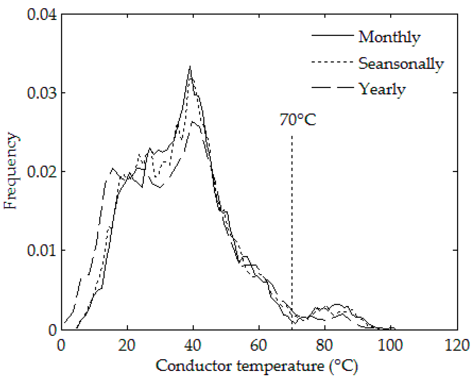
When the yearly, seasonally and monthly ratings under 99% confidence level (Table 2) flow through the line, the frequency distribution of conductor temperature is shown in Figure 8. In the operating year, the maximum, average and minimum values of the conductor temperature corresponding to the yearly rating are 96.2 °C, 35.0 °C and 0.06 °C, respectively. Similarly, the temperatures corresponding to the seasonally rating are 98.4 °C, 37.5 °C and 4.2 °C, and corresponding to the monthly rating are 102.1 °C, 38.0 °C and 4.4 °C, respectively. The operation risks of yearly, seasonally and monthly ratings are 3.07%, 4.53% and 4.99% shown in Table 4. Compared with STR, the yearly rating and the average of the seasonally and monthly ratings increased by 51.86%, 61.23% and 62.78% respectively. From Figure 8 and Table 4, it can be seen that the QDR of the line increases greatly with the decrease of the time scale. However, the operation risk increases slightly, which further illustrates the necessity of shortening the time scale of the thermal rating.
Figure 9 shows the operation risks of QDR under different time scales and confidence levels (90% to 99%, increasing by 1%). When the confidence level is 99%, the yearly rating and the average of seasonally and monthly ratings are 899 A, 954.5 A and 963.67 A, and the operation risks are 3.07%, 4.53% and 4.99%, respectively. Similarly, the ratings are 1314 A, 1364.75 A and 1377.92 A under the confidence level of 90%, and the operation risks are 27.89%, 28.76% and 29.26%, respectively. Obviously, the QDR and operation risk increase with the decrease of the confidence level. Accordingly, the confidence level has a great impact on operation risk. It is worth mentioning that the randomness of meteorological parameters, such as wind speed and ambient temperature, is the main cause of operational risk. If the historical meteorological data and operational meteorological data are identical, the operation risk only depends on the confidence level. Specifically, when the confidence level is 99%, the operation risk is 1%, regardless of conductor’s own characteristic parameters, such as the absorptivity, emissivity or the diameter.
Assuming that the line studied will in service for 12 years with the operation meteorological data, the time series of high conductor temperature and corresponding exposure time can be obtained. The conductor tension loss at a certain temperature can be calculated by Equation (6), taking into account its exposure time. Then the tension loss at all temperatures is accumulated. The risk of the 99% confidence level thermal rating is small, and its tension loss is very small when operate for 12 years. The time series of high conductor temperature (above 95 °C) and corresponding exposure time under the thermal rating of 98% confidence level are shown in Table 5. The cumulative process of the total loss of tensile strength of aluminum strands is illustrated in Figure 10. As shown in Figure 10, the loss of tensile strength of an individual aluminum strand is LAl = 4.88%.
Since LGJ-400/50 conductor is a composite conductor that has a steel core, its overall loss of tensile is substantially reduced. The total loss of tensile strength in a composite conductor is computed using Equations (7)–(9). The single-core aluminum conductor tensile loss of 4.88% is converted to the tension loss of the composite conductor, which is 2.63%. Table 6 shows the tension loss for yearly, seasonally and monthly rating at different confidence levels for a duration of 12 years. The lower the confidence level is, the higher the thermal rating, and the more serious the tension loss is. In Table 6, the tension loss of confidence level below 95% confidence level is not given, because the corresponding tension loss exceeds the allowable value of 15%. QDR can improve the utilization of current carrying capacity a of transmission lines, but there is also the risk of operating at too high conductor temperature. The resulting conductor tension loss will affect the service life of transmission lines. The confidence level is an important parameter affecting QDR and operational risk, and its accurate selection is very important. In this paper, three suggestions are given: first, to improve the utilization of the line as much as possible; second, the conductor temperature should not reach 120 °C; third, the economic benefit and operation cost of the whole life cycle of the line should be considered.
6. Discussion
Because the QDR technology has not been implemented in Weihai, in the absence of meteorological data along the transmission line, this paper regards the transmission line as a lumped element and presents a quasi-dynamic rating analysis. In fact, meteorological conditions can differ along the power line. The study line is the longest transmission line with the length of 47 km in Weihai, from Weihai to Wendeng. The above QDR are calculated using Weihai meteorological data. For comparison, the DTR and QDR are calculated with the meteorological data (wind speed and ambient temperature) of Wendeng at the end of the line. In practice, the wind direction of each point along the overhead line is different, and the direction of the overhead transmission line is also changing. Therefore, the angle between the wind direction and the line axis, that is, the angle of wind incidence, is very different in different positions of the line. Wind incidence angle has great randomness in time and space distribution. Therefore, the long-term average of wind incidence angle of 45° is adopted in this paper. The results of DTR and QDR under Weihai and Wendeng meteorological data are compared. The results show that the average difference of DTR is 319.5 A, while the difference of QDR is small. The difference of average monthly rating, seasonally rating and yearly rating are 46 A, 45 A and 54 A at the confidence level of 99%, respectively. This further shows that in the absence of along-line measuring devices, QDR is more accurate, reliable and cost-saving. In addition, the transmission line is regarded as a lumped parameter element for simplified conditions, and the QDR is calculated theoretically based on the heat balance equation rather than experimental verification, which is the limitation of this paper. In practical application, the optimal arrangement of meteorological sensors and their sampling resolution, and the specific topography, sag and the key span along the line need to be considered.
7. Conclusions
Based on the change of key parameters, a method for driving long time scale QDR is proposed in this paper. By statistical analysis of the maximum allowable ampacity, the QDR under different time scales and confidence levels is determined, which effectively increases the utilization of line capacity on the basis of saving the cost of monitoring. In this paper, through control variate method, the key parameters affecting the ampacity are accurately identified as wind speed, ambient temperature and wind direction. Key parameters, confidence level and time scale are important factors affecting QDR. With the decrease of confidence level and time scale, the results of QDR are increased. Therefore, with the permission of operation and control complexity, shortening the time scale of QDR can effectively improve the utilization of transmission lines. Moreover, the tension loss should be taken into account in the selection of confidence level. When the temperature of aluminium conductor exceeds 120°C, its aging speed will become very fast. The optimal confidence level should be selected to maximize the utilization of current carrying capacity under the condition that the conductor temperature does not exceed 120°C, and the economic benefits and operating costs under the whole life cycle should also be taken into account in future work.
Author Contributions
Conceptualization, Y.W.; methodology and data, F.S. and H.Y.; writing—original draft preparation, F.S.; writing—review and editing, X.Z. and Z.N.
Funding
This research was funded by the National Natural Science Foundation of China, grant number 51607107 and 51641702, the Science and Technology Development Project of Shandong Province, China, grant number ZR2015ZX045, and the Science and Technology Development Project of Weihai City, grant number 2018DXGJ05.
Conflicts of Interest
The authors declare no conflict of interest.
References
- Teh, J.; Ooi, C.A.; Cheng, Y.H. Composite reliability evaluation of load demand side management and dynamic thermal rating systems. Energies 2018, 11, 466. [Google Scholar] [CrossRef]
- Dawson, L.; Knight, A.M. Applicability of dynamic thermal line rating for long lines. IEEE Trans. Deliv. 2018, 33, 719–727. [Google Scholar] [CrossRef]
- Teh, J.; Lai, C.M.; Muhamad, N.A. Prospects of using the dynamic thermal rating system for reliable electrical networks: A review. IEEE Access 2018, 6, 26765–26778. [Google Scholar] [CrossRef]
- Fan, F.; Bell, K.; Infield, D. Transient-state real-time thermal rating forecasting for overhead lines by an enhanced analytical method. Electr. Power Syst. Res. 2019, 167, 213–221. [Google Scholar] [CrossRef]
- Cong, Y.; Regulski, P.; Wall, P. On the use of dynamic thermal-line ratings for improving operational tripping schemes. IEEE Trans. Power Deliv. 2016, 31, 1891–1900. [Google Scholar] [CrossRef]
- Ngoko, B.O.; Sugihara, H.; Funaki, T. A short-term dynamic thermal rating for accommodating increased fluctuations in conductor current due to intermittent renewable energy. Asia-Pac. Energy Eng. Conf. (APPEEC) 2016, 141–145. [Google Scholar] [CrossRef]
- Greenwood, D.M.; Gentle, J.P.; Smyers, K. A comparison of real-time thermal rating systems in the U.S. and the U.K. IEEE Trans. Power Deliv. 2014, 29, 1849–1858. [Google Scholar] [CrossRef]
- Michiorri, A.; Nguyen, H.M.; Alessandrini, S. Forecasting for dynamic line rating. Renew. Sustain. Energy Rev. 2015, 52, 1713–1730. [Google Scholar] [CrossRef] [Green Version]
- Zhan, J.; Chung, C.Y.; Demeter, E. Time series modeling for dynamic thermal rating of overhead lines. IEEE Transm. Power Syst. 2017, 32, 2172–2182. [Google Scholar] [CrossRef]
- Teh, J.; Cotton, I. Critical span identification model for dynamic thermal rating system placement. IET Gener. Transm. Distrib. 2015, 9, 2644–2652. [Google Scholar] [CrossRef]
- Kosec, G.; Maksić, M.; Djurica, V. Dynamic thermal rating of power lines—Model and measurements in rainy conditions. Int. J. Electr. Power Energy Syst. 2017, 91, 222–229. [Google Scholar] [CrossRef]
- Hosek, J.; Musilek, P.; Lozowski, E. Effect of time resolution of meteorological inputs on dynamic thermal rating calculations. IET Gener. Transm. Distrib. 2011, 5, 941–947. [Google Scholar] [CrossRef]
- Increased Power Flow through Transmission Circuits: Overhead Line Case Studies and Quasi-Dynamic Rating; Tech. Rep. 1012533; Electric Power Research Institute (EPRI): Palo Alto, CA, USA, 2006.
- Mahmoudian Esfahani, M.; Yousefi, G.R. Real time congestion management in power systems considering quasi-dynamic thermal rating and congestion clearing time. IEEE Trans. Ind. Inf. 2016, 12, 745–754. [Google Scholar] [CrossRef]
- Wang, Y.L.; Yan, Z.J.; Liang, L.K. Dynamic rating analysis of overhead line loadability driven by meteorological data. Power Syst. Technol. 2018, 42, 315–321. [Google Scholar] [CrossRef]
- CIGRE WG22.12. Thermal behavior of overhead conductors. Electra 1992, 144, 107–125. [Google Scholar]
- IEEE Standard 738. IEEE standard for calculating the current-temperature relationship of bare overhead conductors. IEEE 2012. [Google Scholar] [CrossRef]
- Teh, J.; Lai, C.M.; Cheng, Y.H. Improving the penetration of wind power with dynamic thermal rating system, static VAR compensator and multi-objective genetic algorithm. Energies 2018, 11. [Google Scholar] [CrossRef]
- Musilek, P.; Heckenbergerova, J.; Bhuiyan, M.M.I. Spatial analysis of thermal aging of overhead transmission conductors. IEEE Trans. Power Deliv. 2012, 27, 1196–1204. [Google Scholar] [CrossRef]
- Bočkarjova, M.; Andersson, G. Transmission line conductor temperature impact on state estimation accuracy. In Proceedings of the 2007 IEEE Lausanne Power Tech, Lausanne, Switzerland, 1–5 July 2007. [Google Scholar] [CrossRef]
- Rahman, M.; Kiesau, M.; Cecchi, V. Investigating the impacts of conductor temperature on power handling capabilities of transmission lines using a multi-segment line model. SoutheastCon 2017. [Google Scholar] [CrossRef]
- Heckenbergerová, J.; Musilek, P.; Filimonenkov, K. Quantification of gains and risks of static thermal rating based on typical meteorological year. Int. J. Electr. Power Energy Syst. 2013, 44, 227–235. [Google Scholar] [CrossRef]
Figure 1.
Wind speed frequency distribution histogram (June 2009 to June 2017).

Figure 2.
Ambient temperature frequency distribution histogram (June 2009 to June 2017).

Figure 3.
Wind incidence angle frequency distribution histogram in 2015.

Figure 4.
The LGJ-400/50 line.

Figure 5.
Ampacity with the interval of 10 min (June 2009 to June 2017).

Figure 6.
QDR under different time scales (99% confidence level).

Figure 7.
Conductor temperature under different wind speeds and ambient temperatures (I = 899 A).

Figure 8.
Conductor temperature frequency distribution of QDR under different time scales (99% confidence level).
Figure 8.
Conductor temperature frequency distribution of QDR under different time scales (99% confidence level).

Figure 9.
The operation risks of QDR under different time scales and confidence levels.

Figure 10.
Determination of the loss of tensile strength of an individual aluminum strand (98% confidence level).
Figure 10.
Determination of the loss of tensile strength of an individual aluminum strand (98% confidence level).


Table 1.
Influence of parameters on ampacity.
| Order | Parameters | Ampacity Difference | Influence Degree |
|---|---|---|---|
| 1 | wind speed | 1792.0 | high |
| 2 | ambient temperature | 752.7 | high |
| 3 | wind incidence angle | 621.1 | high |
| 4 | emissivity | 78.6 | low |
| 5 | sunshine intensity | 62.7 | low |
| 6 | solar hour angle | 50.0 | low |
| 7 | solar absorptivity | 42.1 | low |
| 8 | declination angle | 34.1 | low |
Table 2.
QDR under different time scales (99% confidence level).
| Time Scale | QDR (A) | Time Scale | QDR (A) |
|---|---|---|---|
| year | 899 | ||
| spring | 945 | Mar. | 1048 |
| Apr. | 926 | ||
| May | 913 | ||
| summer | 842 | Jun. | 881 |
| Jul. | 835 | ||
| Aug. | 820 | ||
| autumn | 934 | Sept. | 872 |
| Oct. | 964 | ||
| Nov. | 1014 | ||
| winter | 1097 | Dec. | 1096 |
| Jan. | 1107 | ||
| Feb. | 1088 |
Table 3.
Yearly and seasonally ratings under different confidence levels.
| Confidence Level | Yearly Rating (A) | Spring Rating (A) | Summer Rating (A) | Autumn Rating (A) | Winter Rating (A) |
|---|---|---|---|---|---|
| 90% | 1314 | 1378 | 1190 | 1328 | 1563 |
| 91% | 1294 | 1356 | 1169 | 1308 | 1541 |
| 92% | 1273 | 1332 | 1146 | 1286 | 1516 |
| 93% | 1248 | 1304 | 1119 | 1262 | 1485 |
| 94% | 1219 | 1270 | 1087 | 1234 | 1452 |
| 95% | 1181 | 1231 | 1046 | 1198 | 1412 |
| 96% | 1135 | 1180 | 996 | 1153 | 1359 |
| 97% | 1082 | 1119 | 931 | 1091 | 1290 |
| 98% | 1005 | 1056 | 878 | 1019 | 1214 |
| 99% | 899 | 945 | 842 | 934 | 1097 |
Table 4.
Rating results analysis under 99% confidence level.
| Rating Mode | Mean Value of Thermal Rating (A) | Increase of Ampacity (% of STR) | Operation Risk |
|---|---|---|---|
| STR | 592 | 0 | 0 |
| yearly | 899 | 51.86 | 3.07% |
| seasonally | 954.5 | 61.23 | 4.53% |
| monthly | 963.67 | 62.78 | 4.99% |
Table 5.
Time series of conductor temperature and exposure time.
| Temp (°C) | 96 | 97 | 98 | 99 | 100 | 101 | 102 | 103 | 104 | 105 | 106 | 107 | 108 | 109 | 110 |
|---|---|---|---|---|---|---|---|---|---|---|---|---|---|---|---|
| Hrs (h) | 154 | 148 | 238 | 176 | 174 | 134 | 94 | 58 | 62 | 38 | 24 | 4 | 16 | 14 | 4 |
Table 6.
Total loss of tensile strength operating at different value with various confidence level.
| Confidence Level | Loss of Tensile Strength in a Composite Conductor Lc | ||
|---|---|---|---|
| Yearly | Seasonally | Monthly | |
| 96% | 6.55% | 10.94% | 10.98% |
| 97% | 5.64% | 8.97% | 9.4% |
| 98% | 2.63% | 4.79% | 5.14% |
| 99% | 0.08% | 0 | 0 |
© 2019 by the authors. Licensee MDPI, Basel, Switzerland. This article is an open access article distributed under the terms and conditions of the Creative Commons Attribution (CC BY) license (http://creativecommons.org/licenses/by/4.0/).
Share and Cite
MDPI and ACS Style
Song, F.; Wang, Y.; Yan, H.; Zhou, X.; Niu, Z. Increasing the Utilization of Transmission Lines Capacity by Quasi-Dynamic Thermal Ratings. Energies 2019, 12, 792. https://doi.org/10.3390/en12050792
AMA Style
Song F, Wang Y, Yan H, Zhou X, Niu Z. Increasing the Utilization of Transmission Lines Capacity by Quasi-Dynamic Thermal Ratings. Energies. 2019; 12(5):792. https://doi.org/10.3390/en12050792
Chicago/Turabian StyleSong, Fan, Yanling Wang, Hongbo Yan, Xiaofeng Zhou, and Zhiqiang Niu. 2019. "Increasing the Utilization of Transmission Lines Capacity by Quasi-Dynamic Thermal Ratings" Energies 12, no. 5: 792. https://doi.org/10.3390/en12050792
Note that from the first issue of 2016, this journal uses article numbers instead of page numbers. See further details here.