Emission-Intensity-Based Carbon Tax and Its Impact on Generation Self-Scheduling

Abstract

We propose an emission-intensity-based carbon-tax policy for the electric-power industry and investigate the impact of the policy on thermal generation self-scheduling in a deregulated electricity market. The carbon-tax policy is designed to take a variable tax rate that increases stepwise with the increase of generation emission intensity. By introducing a step function to express the variable tax rate, we formulate the generation self-scheduling problem under the proposed carbon-tax policy as a mixed integer nonlinear programming model. The objective function is to maximize total generation profits, which are determined by generation revenue and the levied carbon tax over the scheduling horizon. To solve the problem, a decomposition algorithm is developed where the variable tax rate is transformed into a pure integer linear formulation and the resulting problem is decomposed into multiple generation self-scheduling problems with a constant tax rate and emission-intensity constraints. Numerical results demonstrate that the proposed decomposition algorithm can solve the considered problem in a reasonable time and indicate that the proposed carbon-tax policy can enhance the incentive for generation companies to invest in low-carbon generation capacity.

1. Introduction

Thermal-power generation is one of the main sources of carbon dioxide emissions. About 41 percent of global carbon dioxide emissions come from thermal-power generation. Since excessive emission of carbon dioxide leads to global warming and environmental deterioration, it is important to set up a reasonable policy to reduce carbon dioxide emissions from thermal-power generation for the sustainable development of the electric-power industry.

1.1. Literature Review

Three policies are generally implemented to reduce emissions from the electric power industry. The first policy is the emissions-cap policy that specifies a limit or cap on the total quantity of emissions over a certain time period. Related studies include an emission-constrained typical unit commitment problem [1], a tabu search and Benders decomposition based short term unit commitment solution approach [2], emission-constrained generation self-scheduling problems [3,4], the emission-constrained robust self-scheduling of a hydro-thermal generation company [5], a stochastic long-term security-constrained unit commitment formulation [6], and the stochastic self-scheduling of thermal units with emission constraints [7]. The second policy is the emissions-trading scheme (ETS) that allocates each emission entity a specified emission allowance, and allows emission entities to purchase or sell allocated allowances in the emissions-trading market. The ETS was first introduced in European Union [8] and then developed in many other countries. The effects of the ETS on generation scheduling were studied in [9]. Emissions-trading planning for a combined heat and power producer was investigated in [10]. The impacts of the ETS on the Nordic electricity market and electricity consumers were assessed in [11]. An agent-based model was established in [12] to study the potential impact of carbon-emissions trading on the power sector in China. Fuel switching in electricity production under the ETS was discussed in [13]. A computable general equilibrium model was established in [14] to analyze the impact of carbon-allowance allocation on the electric-power industry in China. A review of the carbon-trading market in China was presented in [15]. The third policy is the carbon-tax policy, under which generation companies are obliged to pay for their carbon dioxide emissions according to the carbon-tax rate and the quantity of their emissions. The carbon-tax policy was first implemented in Finland and gradually spread in many other countries, such as Sweden, Denmark, and Germany. A revenue and distributionally neutral approach was described in [16] to design a carbon tax to reduce greenhouse-gas emissions. The mitigation effects of carbon tax on carbon dioxide emissions are comprehensively estimated in [17]. A carbon tax generation self-scheduling model was presented and the effects of generation profits and emissions profiles under different carbon-tax scenarios are analyzed in [18]. Different evolutions of carbon dioxide taxes that might be applied to the national electricity sector in Portugal were studied in [19]. A choice experiment study of Chinese companies was summarized in [20] to measure the choice preferences of Chinese companies to carbon-tax policy. A bibliometric analysis of the carbon-tax literature from 1989 to 2014 was provided in [21].

The emissions-cap policy has the advantage of regulating the total quantity of emissions, but lacks impetus from market forces. The ETS has the advantages of broad participation, international equity, and controlling the total quantity of emissions [22], but has to face the impact of large uncertainties from emissions-trading platforms on policy efficiency [16]. Compared with the emissions-cap policy and the ETS, the carbon-tax policy not only provides a price signal to impel emitters to develop low-carbon technologies or cleaner energy sources [23], but can also be implemented without trading platforms; consequently, it is highly recommended by economists and organizations [17].

1.2. Work and Contribution of the Paper

A challenge of carbon-tax policy is how to determine the tax rate, which is the levied charge per unit quantity of emissions. If the tax rate is low, emissions cannot be effectively reduced. If the tax rate is high, both production and economic profits are badly hurt. In the previous literature, the tax rate is usually a designated constant [18,24,25]. However, the use of a constant tax rate does not take into account the difference in pollution levels between generation companies, and lacks flexibility in incentives to reduce emissions. It was indicated in [26] that changing the tax rate based on energy efficiency is more effective than applying the same tax rate to all manufacturers. It was suggested in [27] to allow the tax rate to vary among generation units.

Inspired by the idea in [26,27], we propose in this paper an emission intensity-based carbon tax policy in the context of the electric-power industry. Emission intensity is the quantity of emissions per unit power generation. It is an index to measure the pollution level of power generation. The higher emission intensity is, the more serious the pollution in power generation is. In order to improve controlling power-generation pollution, and impel generation companies to invest in low-carbon power generation, we provide different carbon-price signals for different power-generation levels. That is, we adjust the tax rate according to the pollution level of power generation. The more serious the pollution in power generation is, the higher the assigned tax rate is. Therefore, the tax rate is designed to stepwise increase as emission intensity of power generation increases. By introducing emission intensity, the proposed carbon-tax policy increases taxation on high pollution production while balancing generation contribution and environmental pollution in determining the tax rate.

To analyze the effect of the proposed carbon-tax policy, we investigate the impact of the policy on generation self-scheduling decisions. The generation self-scheduling problem plays an important role in the daily-operation planning of generation companies in the deregulated electricity market. A typical generation self-scheduling problem is deciding the operation of generation units according to electricity prices and the physical characteristics of generation units, with the objective of maximizing total profits [28,29]. Effective generation self-scheduling can promote the economic operation of generation companies. Under the proposed carbon-tax policy, generation companies need to not only adjust power output according to price signal, but also reduce emissions according to the carbon-tax policy, which brings a new challenge for generation self-scheduling decisions.

Our work is different from [26,27] in the following two aspects. First, the mechanisms for designing the tax rate are different. The tax rate was designed based on game theory in both [26] and [27], while it is designed by explicitly formulating the relation function between tax rate and emission intensity in our work. Second, the involved models are different. A simple numerical example was considered in [26], a simplified economic dispatch model omitting time-coupled unit-operation constraints was considered in [27], while an explicit generation self-scheduling model that includes conventional unit-operation constraints and decides not only economic dispatch but also unit commitment is considered in our work. A tax rate that varies based on the quantity of emissions was presented in [30]. Our work is different from [30] in that tax-rate variation in our work is emission intensity-based. Compared with [30], our work in determining tax rate takes into account not only generation emissions but also generation contribution. The major contributions of the paper can be summarized as follows:

(1)

A carbon-tax policy with variable tax rate is proposed with regard to the electric-power industry. Tax rate is designed to increase stepwise with the increase of power-generation emission intensity, which can strengthen tax collection from high-pollution generation companies and balance electricity supply and environmental pollution in determining tax rate.

(2)

The impact of the proposed carbon-tax policy is investigated by formulating the generation self-scheduling problem under the proposed carbon-tax policy as a mixed integer nonlinear programming (MINLP) model and developing a decomposition algorithm to solve the problem.

(3)

Numerical experiments are carried out to test the performance of the proposed algorithm and discuss the effectiveness of the proposed carbon tax policy.

The remainder of this paper is organized as follows: Formulation of the generation self-scheduling problem under the proposed carbon-tax policy is described in Section 2. The solution approach to solving this problem is developed in Section 3. Numerical experiments and results are presented in Section 4. The conclusions of the paper are provided in Section 5.

2. Problem Description and Formulation

2.1. Parameteres and Decision Variables

The parameters and decision variables used in the formulation are defined as follows:

Parameters

n	Number of generation units.
T	Scheduling horizon.
M	Number of carbon-tax rate values.
${\tau }_i^D/{\tau }_i^U$	Minimum down-time/up-time of generation unit i.
$R_i^D/R_i^U$	Ramp-down/ramp-up rate of generation unit i.
$S_i^D/S_i^U$	Shutdown/startup ramp rate of generation unit i.
$P_i^L/P_i^U$	Minimum/maximum power output of generation unit i.
${\alpha }_{ih}/{\beta }_{ih}$	Slope/intercept of the h-th segment line for the fuel-cost curve of generation unit i.
$B_i$	Startup cost of generation unit i.
$r_i$	Emission coefficient of generation unit i.
$\mu$	Emission intensity.
$\rho$	Carbon-tax rate.
$w_m$	The m-th carbon-tax rate value.
$Q_m$	Upper bound of emission intensity corresponding to the m-th carbon-tax rate value.
${\lambda }_t$	Expected electricity price in hour t.
$u_{i0}$	Binary parameter to indicate the initial on/off status of generation unit i.
$p_{i0}$	Generation output of generation unit i in hour 0.
${\sigma }_i$	Last hour of the periods during which the on/off status of generation unit i is determined by the initial status of the generation unit.

Decision Variables

$u_{it}$	Binary decision variable to indicate on/off status of generation unit i in hour t.
$v_{it}$	Binary decision variable to indicate if generation unit i is started up in hour t.
$p_{it}$	Generation output of generation unit i in hour t.
${\varphi }_{it}$	Fuel cost of generation unit i in hour t.
${\delta }_m$	Binary decision variable to indicate whether carbon-tax rate equals m-th carbon-tax rate value.

2.2. Description and Formulation of Carbon-Tax Policy

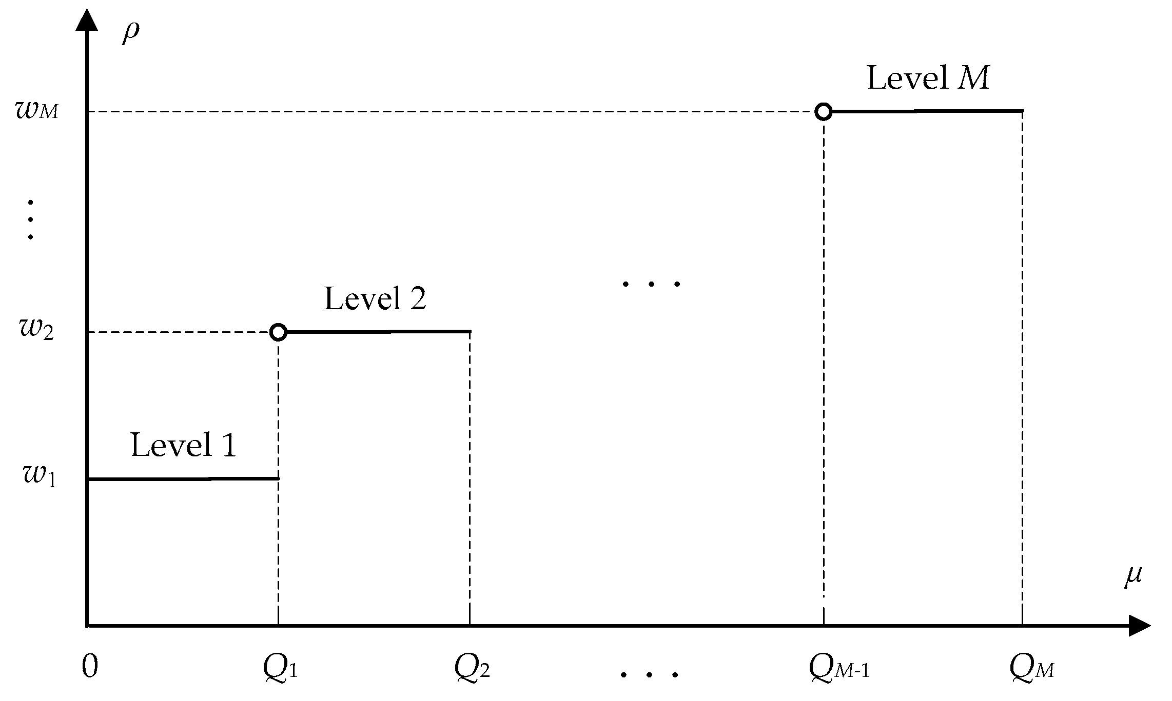
For the carbon tax policy, we consider M levels for the tax rate as illustrated in Figure 1. Each level corresponds to a tax-rate value and a range of emission intensity. Each tax rate value provides a carbon-tax signal for the corresponding emission-intensity range.

Tax rate is variable and equals a tax-rate value according to the range to which emission intensity belongs. The relationship between tax rate and emission intensity can be formulated by a step-up function as follows:

$$\rho =\{\begin{array}{ll}{w}_1,\hfill & \mu \le Q_1\hfill \\ w_m,\hfill & Q_{m-1}<\mu \le Q_m,m=2,\dots ,M-1\hfill \\ w_M,\hfill & \mu >Q_{M-1}\hfill \end{array}$$

(1)

where $0\le w_1\le w_2\le \cdots \le w_M$, and emission intensity μ over the scheduling horizon is determined by the ratio of the quantity of total emissions [1,9] to the total generation level as follows:

$$\mu =\{\begin{array}{l}{\displaystyle \sum _{i=1}^n{\displaystyle \sum _{t=1}^T{r}_i{\varphi }_{it}}}/{\displaystyle \sum _{i=1}^n{\displaystyle \sum _{t=1}^T{p}_{it}}},\mathrm{if}{\displaystyle \sum _{i=1}^n{\displaystyle \sum _{t=1}^T{p}_{it}}}>0\hfill \\ 0,\mathrm{otherwise}\hfill \end{array},$$

(2)

$0<Q_1<Q_2<\cdots <Q_{M-1}<Q_M$, and $Q_M$ is the upper bound of possible emission intensity. Expression (1) shows that tax rate increases stepwise as emission intensity increases. Particularly, when M = 1, the tax rate is constant. Therefore, the proposed carbon tax policy is a generalization of the typical carbon tax policy with a constant tax rate.

2.3. Generation Self-Scheduling Model under the Proposed Carbon-Tax Policy

To investigate the effect of the proposed carbon tax policy, we consider the generation self-scheduling problem under the proposed carbon-tax policy, which is described as follows. A generation company schedules a certain number of thermal generation units and sells the produced electricity at the market price. The objective is to maximize generation profits. The generation company is obliged to pay for generation emissions in accordance with the proposed carbon-tax policy. The scheduling of generation units needs to satisfy operating constraints such as minimum up-time and down-time constraints, generation-capacity constraints, and ramp-rate constraints.

Based on the above description, the generation self-scheduling problem under consideration can be formulated as follows:

(P)

$$\max {\displaystyle \sum _{t=1}^T{\lambda }_t{\displaystyle \sum _{i=1}^n{p}_{it}}}-{\displaystyle \sum _{i=1}^n{\displaystyle \sum _{t=1}^T({\varphi }_{it}+B_i{v}_{it})}}-\rho {\displaystyle \sum _{i=1}^n{\displaystyle \sum _{t=1}^T{r}_i{\varphi }_{it}}}$$

(3)

subject to (1), (2), and:

$$u_{it}=u_{i0},\forall i,t=1,\dots ,{\sigma }_i$$

(4)

$$v_{it}=0,\forall i,t=1,\dots ,{\sigma }_i$$

(5)

$$u_{it}-u_{i,t-1}\le u_{ik},\forall i,k=t+1,\dots ,\min \{T,{\tau }_i^U+t-1\},t={\sigma }_i+1,\dots ,T$$

(6)

$$u_{i,t-1}-u_{it}\le 1-u_{ik},\forall i,k=t+1,\dots ,\min \{T,{\tau }_i^D+t-1\},t={\sigma }_i+1,\dots ,T$$

(7)

$$u_{it}-u_{i,t-1}\le v_{it},\forall i,t={\sigma }_i+1,\dots ,T$$

(8)

$$u_{it}{P}_i^L\le p_{it}\le u_{it}{P}_i^U,\forall i,\forall t$$

(9)

$$-R_i^D{u}_{i,t+1}-S_i^D(1-u_{i,t+1})\le p_{i,t+1}-p_{it}\le R_i^U{u}_{it}+S_i^U(1-u_{it}),\forall i,t=0,\dots ,T-1$$

(10)

$${\varphi }_{it}\ge {\alpha }_{ih}{p}_{it}+{\beta }_{ih}{u}_{it},\forall h,\forall i,\forall t$$

(11)

$${\varphi }_{it},p_{it}\ge 0,\forall i,\forall t$$

(12)

$$u_{it},v_{it}\in \{0,1\},\forall i,\forall t.$$

(13)

In formulation (P), function (3) represents generation profits, which consist of generation revenue, generation cost, and paid tax for generation emissions. Constraints (4) and (5) represent the impact of the initial statuses of generation units on the on/off statuses, and the start-up actions of generation units over the scheduling horizon, respectively [31,32]. Constraints (6) and (7) represent the minimum up-time and down-time requirements of generation units, respectively. Constraints (8) represent the relationship between the on/off statuses and the start-up actions of generation units. Constraints (9) represent the range of output power for the committed generation units. Constraints (10) define the ramp-rate limits to represent the relationship between output levels in adjacent hours. Constraints (11) represent the piecewise linear approximation of the quadratic fuel cost function. Constraints (12) and (13) provide the value fields of the decision variables.

3. Solution Methodology

Formulation (P) includes continuous variables, integer variables, a piecewise expression in the function (1), and a bilinear term in the objective function (3), which corresponds to an MINLP model and makes it impossible to directly solve the problem by using a commercial solver such as CPLEX. Therefore, it is necessary to develop an efficient algorithm to solve the problem. According to the characteristics of (P), we develop the following decomposition algorithm to solve the problem.

3.1. Reformulation of the Problem

First, by introducing binary variables ${\delta }_m$, $m=1,\dots ,M$, to indicate whether the tax rate equals the m-th value or not, we can obtain the integer linear formulation of the tax rate as follows:

$$\rho ={\displaystyle \sum _{m=1}^M{\delta }_m{w}_m}$$

(14)

where:

$${\displaystyle \sum _{m=1}^M{\delta }_m=1}$$

(15)

$${\delta }_m{\displaystyle \sum _{i=1}^n{\displaystyle \sum _{t=1}^T{r}_i{\varphi }_{it}}}\le {\delta }_m{Q}_m{\displaystyle \sum _{i=1}^n{\displaystyle \sum _{t=1}^T{p}_{it}}},m=1,\dots ,M-1$$

(16a)

$${\delta }_m{\displaystyle \sum _{i=1}^n{\displaystyle \sum _{t=1}^T{r}_i{\varphi }_{it}}}>{\delta }_m{Q}_{m-1}{\displaystyle \sum _{i=1}^n{\displaystyle \sum _{t=1}^T{p}_{it}}},m=2,\dots ,M$$

(16b)

$${\delta }_m\in \{0,1\},\forall m.$$

(17)

Then, based on the above expressions, we can reformulate the considered generation self-scheduling problem as:

(P1)

$$\max {\displaystyle \sum _{t=1}^T{\lambda }_t{\displaystyle \sum _{i=1}^n{p}_{it}}}-{\displaystyle \sum _{i=1}^n{\displaystyle \sum _{t=1}^T({\varphi }_{it}+B_i{v}_{it})}}-{\displaystyle \sum _{m=1}^M{\delta }_m{w}_m}{\displaystyle \sum _{i=1}^n{\displaystyle \sum _{t=1}^T{r}_i{\varphi }_{it}}}$$

(18)

subject to (4)–(13), and (15)–(17).

Finally, according to the formulation of the objective function (18), we replace constraints (16b) with:

$${\delta }_m{\displaystyle \sum _{i=1}^n{\displaystyle \sum _{t=1}^T{r}_i{\varphi }_{it}}}\ge {\delta }_m{Q}_{m-1}{\displaystyle \sum _{i=1}^n{\displaystyle \sum _{t=1}^T{p}_{it}}},m=2,\dots ,M$$

(19)

without changing the optimal solution of (P1).

3.2. Decomposition Algorithm

For an arbitrary m, we can obtain the following formulation by fixing ${\delta }_m=1$ and ${\delta }_{m^{\prime }}=0$, $m^{\prime }\ne m$, in (P1):

(P_m)

$$\max {\displaystyle \sum _{t=1}^T{\lambda }_t{\displaystyle \sum _{i=1}^n{p}_{it}}}-{\displaystyle \sum _{i=1}^n{\displaystyle \sum _{t=1}^T({\varphi }_{it}+B_i{v}_{it})}}-w_m{\displaystyle \sum _{i=1}^n{\displaystyle \sum _{t=1}^T{r}_i{\varphi }_{it}}}$$

(20)

subject to constraints (4)–(13), and:

$${\displaystyle \sum _{i=1}^n{\displaystyle \sum _{t=1}^T{r}_i{\varphi }_{it}}}\le Q_m{\displaystyle \sum _{i=1}^n{\displaystyle \sum _{t=1}^T{p}_{it}}},\mathrm{if}1\le m\le M-1$$

(21a)

$$Q_{m-1}{\displaystyle \sum _{i=1}^n{\displaystyle \sum _{t=1}^T{p}_{it}}}\le {\displaystyle \sum _{i=1}^n{\displaystyle \sum _{t=1}^T{r}_i{\varphi }_{it}}},\mathrm{if}2\le m\le M.$$

(21b)

Formulation (P_m) corresponds to a generation self-scheduling problem with a constant tax rate $w_m$ and emission-intensity constraints (21a) and (21b). It is a mixed integer linear programming (MILP) model and can be solved optimally by a commercial solver if the feasible domain determined by (4)–(13), (21a), and (21b) is not empty.

The above observation motivates us to enumerate all feasible ${\delta }_m$ to decompose (P1) into M subproblems (P_m) and develop the following algorithm:

Step 0

Initialization: set $u\_bes{t}_{it}=p\_bes{t}_{it}=0$ for all $i$ and all $t$, $m=1$, $m\_best=1$, and $f\_best=M_f$ where $M_f$ is a large-enough positive number.

Step 1

Solve (P_m) by calling an MILP solver. If (P_m) can be optimally solved, denote the optimally objective function value as $f_m$. If $f_m<f\_best$, update $f\_best$, $m\_best$, and {$u\_bes{t}_{it}$,$p\_bes{t}_{it}$, $i=1,\dots ,n$, $t=1,\dots ,T$} with $f_m$, $m$, and the optimal unit commitment and economic dispatch decisions of (P_m), respectively.

Step 2

If m = M, set

${\delta }_m=\{\begin{array}{l}1,\mathrm{if}m=m\_best\\ 0,\mathrm{otherwise}\end{array}$

and stop. Otherwise, set $m=m+1$ and go to Step 1.

Using the above algorithm, we can obtain optimal objective function value $f\_best$, and optimal unit commitment and economic dispatch decisions {$u\_bes{t}_{it}$, $p\_bes{t}_{it}$, $i=1,\dots ,n$, $t=1,\dots ,T$} for (P1).

4. Numerical Results

In this section, we present the numerical experiments in four parts. In the first part, we use test cases of different sizes to test the performance of the proposed algorithm. In the second part, we test the impact of tax-rate values on generation self-scheduling and provide a method to choose appropriate tax-rate values. In the third part, we test the effect of the proposed carbon-tax policy on emission reduction. In the fourth part, we compare the proposed carbon-tax policy with carbon-tax policy with a constant tax rate. The test cases are described as follows:

(1) In the first part of the experiments, the scheduling horizon is set to 24, 72, 120, and 168 h, respectively, and the number of generation units is set to 10, 40, 70, and 100, respectively. The combination of the two configurations forms 16 problem sizes. Under each problem size, ten test cases are randomly generated. For each test case, parameters for startup costs and emission coefficients are uniformly generated from the ranges provided in

Table 1. Value ranges for startup costs and emission coefficients.

Parameter (Unit)	Value Range
$B_i$ ($)
If $P_i^U<600$	($4P_i^U$, $6P_i^U$)
If $P_i^U\ge 600$	($2P_i^U$, $4P_i^U$)
$r_i$ (t/$)
If $P_i^U<600$	(0.05, 0.09)
If $P_i^U\ge 600$	(0.005, 0.04)

, in which ranges for startup costs are based on those for cool-start fuel costs in [33] and ranges for emission coefficients are based on data in [9]. Other unit parameters are uniformly generated from ranges provided in [33].

(2) In the remaining three parts of the experiments, the test is performed by using the ten sets of generation-unit data corresponding to the problem size of 10 generation units and 24 h in the first part of the experiments. To clearly show the impact of the proposed carbon-tax policy on generation self-scheduling, the initial status of each generation unit is modified so that the on/off statuses of the generation unit during the scheduling horizon are not affected by the initial status of the generation unit. For each set of generation-unit data, the scheduling horizon is set to 24, 72, 120, and 168 h, respectively. The combination of the generation-unit data and the scheduling horizon forms 40 test cases.

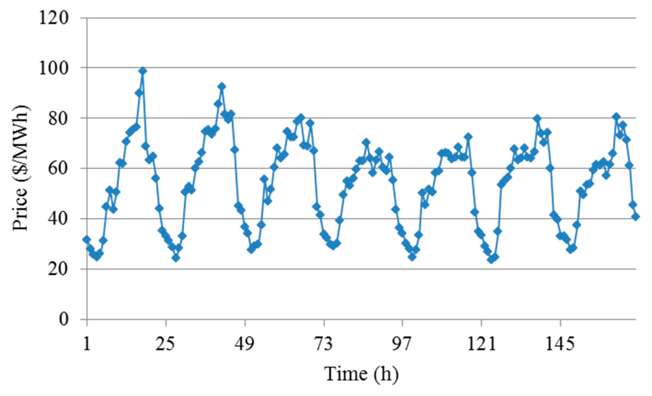
(3) The number of tax rate values can be set according to the actual requirement. If the number of tax rate values is too small, pollution levels cannot be well-distinguished. If the number of tax rate values is too large, it is inconvenient to implement carbon-tax policy. As a tradeoff between the two aspects, the number of tax rate values is set as five in the experiments. Based on the range of emission intensity, $Q_m$ is set to 0.1m and w_m is set to mΔ, in which tax-rate increment Δ is set to 15 without loss of generality in the first part of the experiments; its value is discussed in the second part of the experiments. In practice, tax-rate value w_m can be set in other form according to the requirements. We use Pennsylvania–New Jersey–Maryland (PJM) Interconnection Real Time data from 2005 to 2006 [34] to estimate electricity prices. The estimated price data for 168 h are presented in Figure 2. A ten-piece piecewise linear function is used to approximate each fuel cost function.

The solution algorithm is tested under the computing environment of 3.40 GHz Intel Core i7 CPU and 16.0 GB memory. The MILP involved is solved by calling CPLEX 12.5.

4.1. Performance of Proposed Algorithm

To test the performance of the proposed algorithm, the MILP approach in which (P1) is transformed into an MILP model by using the method in [35] is also used to solve the test cases. The computation time and the number of cases that can be solved optimally are reported in

Table 2. The computation time and the number of cases that can be solved optimally for the MILP approach and the proposed algorithm.

No.	Size (n × T)	MILP		Proposed
		Time (s)	Na	Time (s)	Na
1	10 × 24	1.40	10	1.04	10
2	40 × 24	23.56	10	4.42	10
3	70 × 24	131.35	8	8.76	10
4	100 × 24	136.17	7	14.07	10
5	10 × 72	8.79	10	3.19	10
6	40 × 72	101.60	4	18.03	10
7	70 × 72	149.65	1	38.45	10
8	100 × 72	468.42	3	68.39	10
9	10 × 120	30.47	10	5.97	10
10	40 × 120	365.90	2	42.42	10
11	70 × 120	284.56	2	77.52	10
12	100 × 120	-	0	131.72	10
13	10 × 168	116.63	10	9.74	10
14	40 × 168	363.93	6	64.14	10
15	70 × 168	-	0	116.33	10
16	100 × 168	-	0	288.06	10
Average		-	5	55.77	10

^a The number of cases that can be solved optimally.

, in which each computation time is the average of solvable test cases in the same problem size. If no test cases in a problem size can be solved optimally, the average computation time is not reported for that problem size. The number of cases that can be solved optimally in the same problem size is denoted by N. From Table 2, we can obtain the following observations:

(1) For the MILP approach, the computation time increases exponentially as the problem size increases. All cases can be solved optimally for the problem in small sizes corresponding to 10 × 24, 40 × 24, 10 × 72, 10 × 120 and 10 × 168. Only partial cases can be solved optimally for the problem in medium sizes corresponding to 70 × 24, 100 × 24, 40 × 72, 70 × 72, 100 × 72, 40 × 120, 70 × 120, and 40 × 168. CPLEX is out of memory for all cases for the problem in large sizes corresponding to 100 × 120, 70 × 168, and 100 × 168. The average number of cases that can be solved optimally in the same problem size is 5.

(2) Compared with the MILP approach, the proposed algorithm requires a shorter computation time. All the cases in all problem sizes can be solved optimally by the proposed algorithm. The average computation time is 55.77 s, and the longest computation time is 288.06 s.

The above observations indicate that the proposed algorithm is more effective than the MILP approach for solving the considered problem and can solve the considered test cases in a reasonable time.

4.2. Impact of Tax-Rate Values on Generation Self-Scheduling

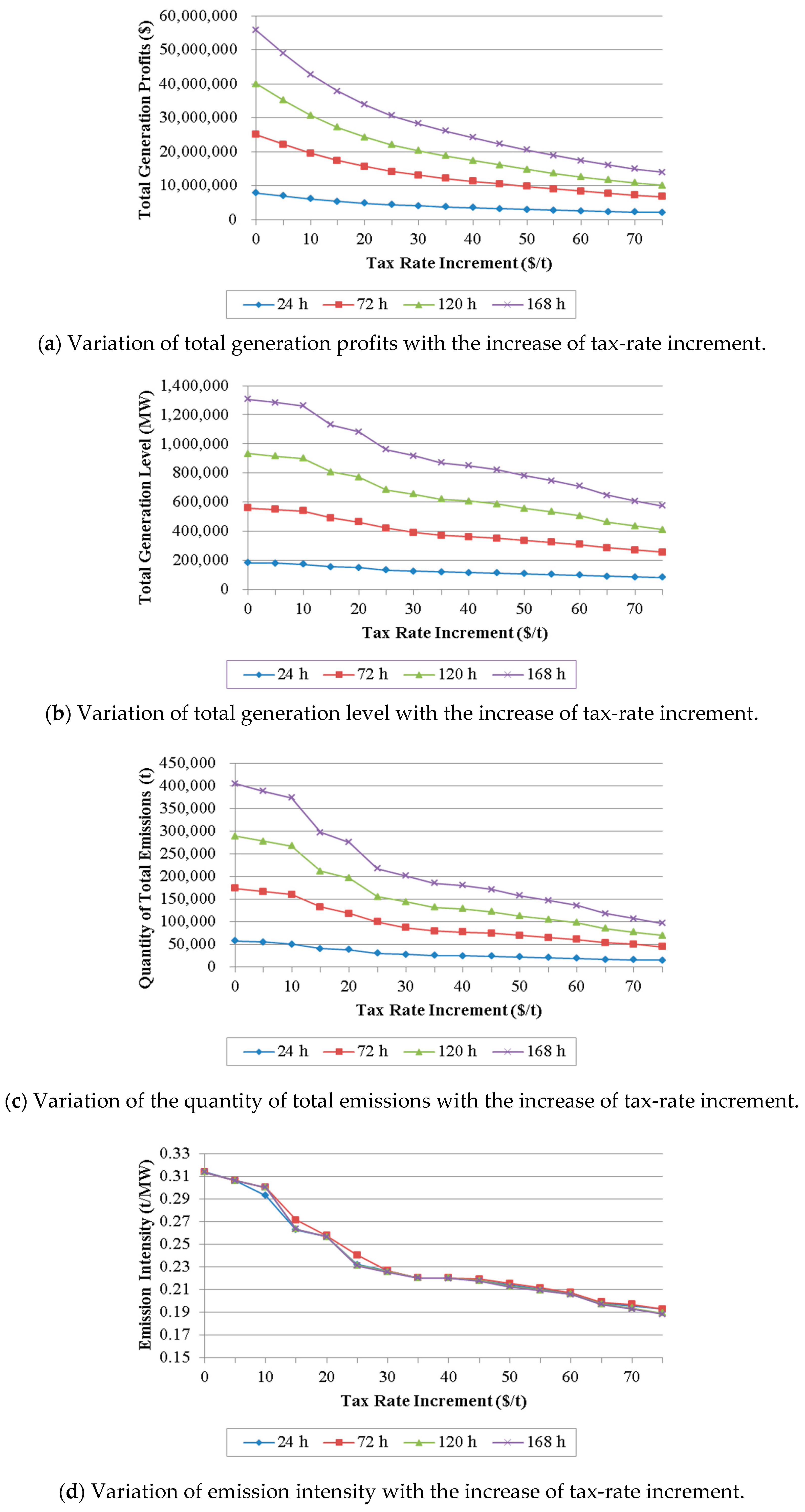
To analyze the impact of the tax-rate values, $w_m$, $m=1,\dots ,5$, on generation self-scheduling, we test the model under different $w_m$ settings by allowing tax-rate increment $\Delta$ to vary within {0, 5, 10, 15, …, 75}. For each tax-rate increment, test cases are solved and four indices are obtained in the optimal solution of each test case, including total profits, total generation level, the quantity of total emissions, and emission intensity over the scheduling horizon. The variations of the four indices, along with the increase of the tax-rate increment, are shown in Figure 3, in which each point depicts the average of the ten test cases in the same problem size. From Figure 3, it can be observed that the four indices show different sensitivity to the change of tax-rate increment as follows:

(1) As tax-rate increment increases, total profits decrease and the sensitivity of the total profits to the tax-rate-increment change gradually decreases.

(2) As tax-rate increment increases, total generation level, the quantity of total emissions, and emission intensity decrease. The decrease rates of the three indices present oscillating behavior when tax-rate increment increases from 0 to 25, and relatively stable behavior when the tax rate increment increases from 25 to 75.

(3) Because emission intensity is the ratio of total emissions quantity to total generation level, the decrease of emission intensity with the increase of tax-rate increment indicates that the quantity of total emissions is more sensitive to the increase of tax-rate increment than total generation level.

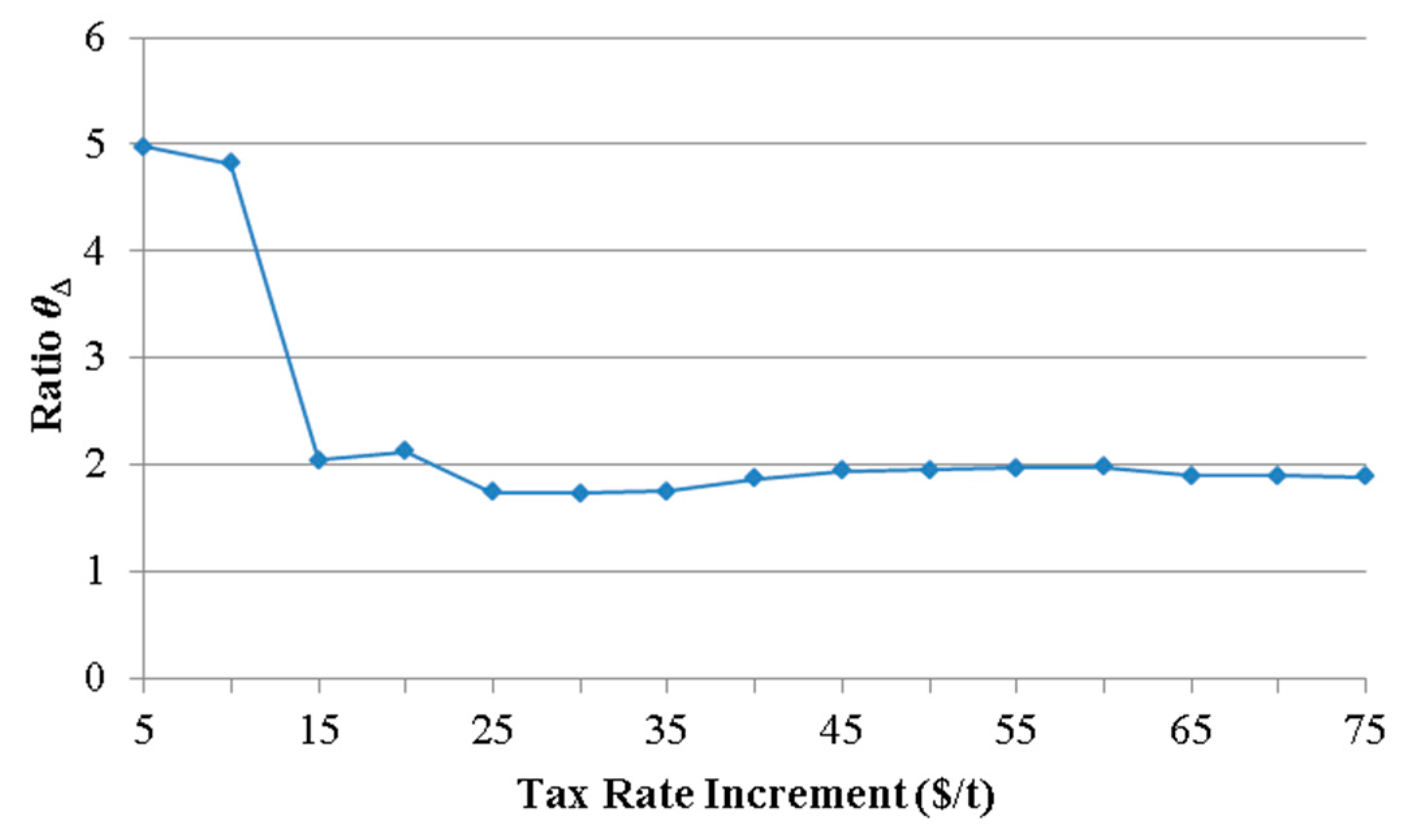
Based on the above observations, we design the following method to choose an appropriate tax-rate increment. Note that a reduction in emission intensity is at the expense of generation profits. To evaluate profit loss in reducing unit emission intensity, we define the ratio of profits-reduction percentage to emission intensity reduction percentage as follows:

$${\theta }_{\Delta }=\frac{(Pro{f}_0-Pro{f}_{\Delta })/Pro{f}_0}{({\mu }_0-{\mu }_{\Delta })/{\mu }_0},$$

in which $Pro{f}_0$ and ${\mu }_0$ are total profits and emission intensity under no carbon-tax policy (corresponding to $\Delta =0$), respectively, and $Pro{f}_{\Delta }$ and ${\mu }_{\Delta }$ are total profits and emission intensity corresponding to a nonzero tax-rate increment $\Delta$, respectively, in which $\Delta \in$ {5, 10, 15, …, 75}. The variation of ${\theta }_{\Delta }$ with the increase of tax-rate increment $\Delta$ is presented in Figure 4, in which each point depicts the average of all test cases. From Figure 4, it can be observed that ${\theta }_{\Delta }$ presents obvious decline behavior when tax-rate increment increases from 5 to 15, reaches the first local minimum value at $\Delta =15$, presents oscillating behavior when tax-rate increment is larger than 15, and reaches the minimum at $\Delta =25$. The difference between ${\theta }_{15}$ and ${\theta }_{25}$ is small. To balance between emission intensity and generation profits, tax-rate increment is set to 15 for the test cases. Correspondingly, tax-rate value $w_m$ is set to $15m$, $m=1,\dots ,5$, which is used in the following experiments.

4.3. Effect of Proposed Carbon Tax Policy on Emission Reduction

To test the effect of the proposed carbon-tax policy on emission reduction, we compare the quantity of total emissions and emission intensity under the proposed carbon-tax policy with those under no carbon-tax policy, respectively. The quantity of total emissions and emission intensity under the proposed carbon-tax policy are reported in columns 4 and 5 of

Table 3. Total generation profits, total generation level, the quantity of total emissions, and emission intensity under the proposed carbon-tax policy.

$\mathit{T}$ (h)	Generation Profits ($)	Generation Level (MW)	Quantity of Emissions (t)	Emission Intensity (t/MW)
24	5,423,040.63	156,285.49	40,663.25	0.26
72	17,369,095.36	491,025.77	131,917.18	0.27
120	27,175,633.46	807,196.34	211,287.38	0.26
168	37,811,819.12	1,131,651.47	296,282.21	0.26
Average	21,944,897.14	646,539.77	170,037.51	0.26

, respectively, and those under no carbon-tax policy are reported in

Table 4. The quantity of total emissions and emission intensity under no carbon-tax policy.

$\mathit{T}$ (h)	Quantity of Emissions (t)	Emission Intensity (t/MW)
24	56,966.69	0.31
72	172,953.10	0.31
120	288,939.50	0.31
168	404,925.90	0.31
Average	230,946.30	0.31

. From the results, we can make the following observations:

(1) For the quantity of total emissions, the average value under the proposed carbon-tax policy is 170,037.51 t, whereas the average value under no carbon-tax policy is 230,946.30 t. The ratio between the two quantities is 0.74. The results show that the quantity of total emissions is reduced by 26% by adopting the proposed carbon-tax policy.

(2) For emission intensity, the average value under the proposed carbon-tax policy is 0.26, whereas the average value under no carbon-tax policy is 0.31. The ratio between the two emission intensities is 0.84. The results show that the quantity of emissions per unit power generation is reduced by 16% by adopting the proposed carbon-tax policy.

The above observations indicate the effectiveness of the proposed carbon-tax policy in reducing total generation emissions and the pollution level of power generation.

4.4. Comparison between Proposed Carbon-Tax Policy and Carbon-Tax Policy with a Constant Tax Rate

To show the difference between the proposed carbon-tax policy and carbon-tax policy with a constant tax rate, we make the following comparisons. First, we compare the optimal solutions under the two carbon-tax policies without changing the test-case parameter setting. Second, we adjust value ranges for emission coefficients and compare the sensitivities of the optimal solutions to the change of emission coefficients under the two carbon-tax policies. For the carbon-tax policy with a constant tax rate, five constant tax rates are considered, with values set from $w_1$ to $w_5$, respectively.

4.4.1. Comparison between Two Carbon-Tax Policies without Changing Parameter Setting

The optimal solution under each carbon-tax policy is presented by the same indices used in Section 4.2. The results under the proposed carbon-tax policy are reported in Table 3, and those under the carbon-tax policy with a constant tax rate corresponding to different settings of the constant tax rate are reported in

Table 5. Total generation profits, total generation level, the quantity of total emissions, and emission intensity under the carbon-tax policy with a constant tax rate.

$\mathit{T}$ (h)	Tax Rate ($/t)	Generation Profits ($)	Generation Level (MW)	Quantity of Emissions (t)	Emission Intensity (t/MW)
24	$w_1$	7,042,972.81	183,806.99	56,954.39	0.31
	$w_2$	6,212,003.63	178,441.98	53,104.73	0.30
	$w_3$	5,453,691.95	168,627.56	47,995.38	0.29
	$w_4$	4,776,296.57	156,731.18	42,564.42	0.28
	$w_5$	4,181,646.67	144,142.39	36,981.80	0.26
72	$w_1$	22,473,333.53	558,384.99	172,915.76	0.31
	$w_2$	19,923,699.57	547,249.87	164,666.40	0.30
	$w_3$	17,556,184.34	522,160.40	150,658.46	0.29
	$w_4$	15,414,841.59	490,051.75	135,105.06	0.28
	$w_5$	13,513,722.19	453,420.58	117,811.99	0.26
120	$w_1$	35,631,936.10	932,979.61	288,892.02	0.31
	$w_2$	31,363,452.90	915,292.42	275,542.84	0.30
	$w_3$	27,399,348.57	873,602.74	251,806.51	0.29
	$w_4$	23,827,289.19	816,426.34	222,986.41	0.28
	$w_5$	20,710,184.75	751,676.87	191,643.08	0.26
168	$w_1$	49,660,909.40	1,307,523.04	404,822.36	0.31
	$w_2$	43,680,701.04	1,282,775.65	386,336.73	0.30
	$w_3$	38,123,525.06	1,224,525.39	353,144.53	0.29
	$w_4$	33,109,787.72	1,145,776.37	313,255.36	0.28
	$w_5$	28,739,390.04	1,053,084.53	268,178.16	0.26
Average	$w_1$	28,702,287.96	745,673.66	230,896.13	0.31
	$w_2$	25,294,964.28	730,939.98	219,912.68	0.30
	$w_3$	22,133,187.48	697,229.02	200,901.22	0.29
	$w_4$	19,282,053.77	652,246.41	178,477.81	0.28
	$w_5$	16,786,235.91	600,581.09	153,653.76	0.26

.

From Table 3 and Table 5, we can make the following observations:

(1) Average emission intensity under the proposed carbon-tax policy is 0.26, which indicates that the average tax rate corresponding to the proposed carbon-tax policy is equal to $w_3$. Compared with the carbon-tax policy with a constant tax rate of no more than $w_3$ ($w_1$, $w_2$, or $w_3$), the proposed carbon-tax policy corresponds to lower generation profits and generation level, but much-reduced emission quantity and intensity.

(2) Compared with the carbon-tax policy with relatively large constant tax rate $w_4$, the proposed carbon-tax policy corresponds to a lower generation level, and emission quantity and intensity, but higher generation profits.

(3) Compared with the carbon-tax policy with the largest constant tax rate $w_5$, the proposed carbon-tax policy is corresponding to higher generation level and quantity of emissions, but an equal emission intensity and much-increased generation profits.

The above comparison indicates the superiority of the proposed carbon-tax policy over the carbon-tax policy with a constant tax rate in comprehensive consideration of generation profits, generation level, emission quantity, and emission intensity.

4.4.2. Comparison between Two Carbon-Tax Policies under Different Emission-Coefficient Settings

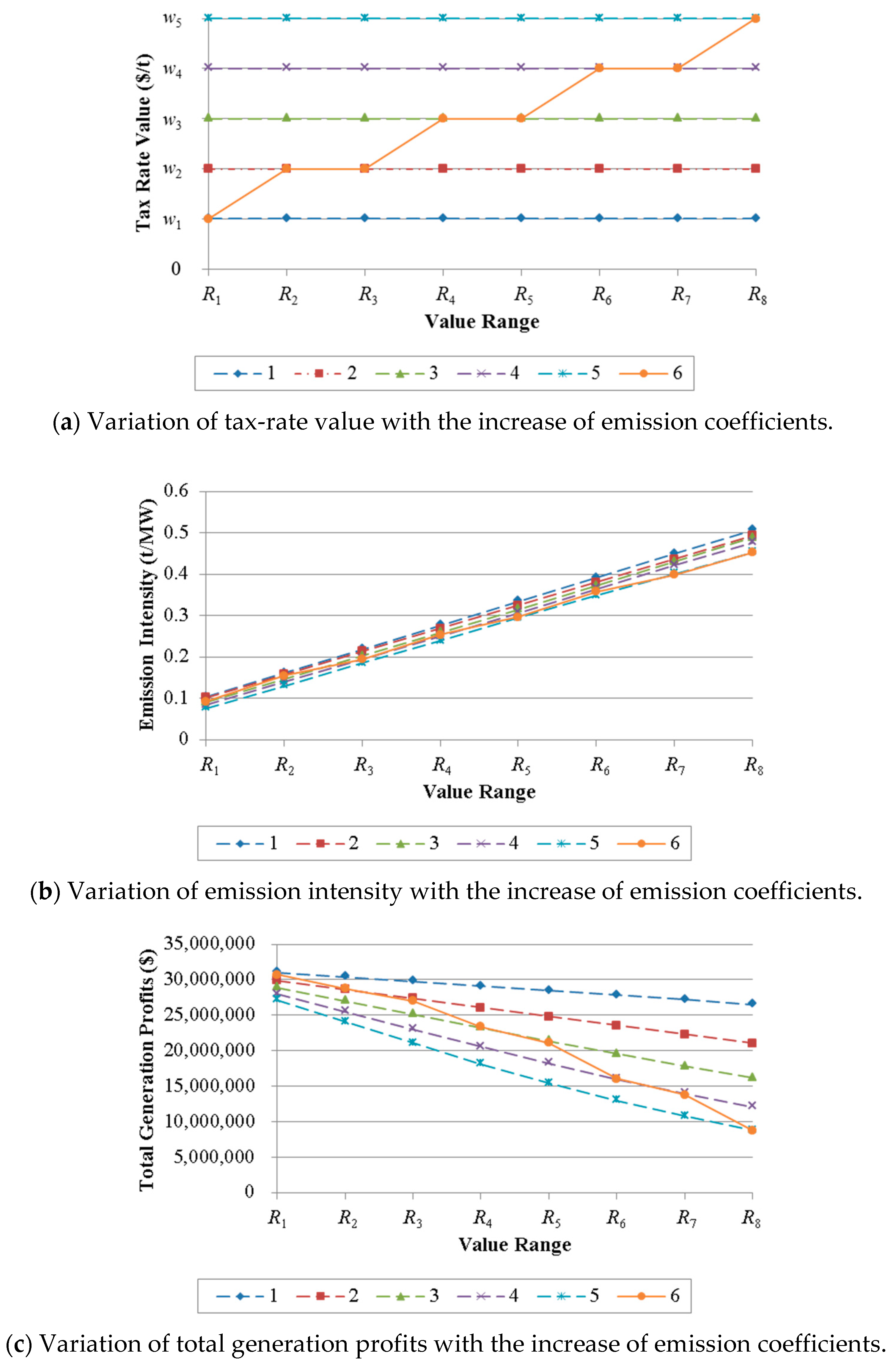
Emission coefficients are important parameters that determine the pollution level of power generation. To show how significantly the optimal solution changes as emission coefficients increase, we test the generation self-scheduling model corresponding to each carbon-tax policy under different value range settings for emission coefficients. In the test, eight sets of value ranges for emission coefficients are considered and provided in

Table 6. Value ranges for emission coefficients.

Situation	${\mathit{R}}_1$	${\mathit{R}}_2$	${\mathit{R}}_3$	${\mathit{R}}_4$
If $P_i^U<600$	(0.05, 0.055)	(0.055, 0.06)	(0.06, 0.065)	(0.065, 0.07)
If $P_i^U\ge 600$	(0, 0.005)	(0.005, 0.01)	(0.01, 0.015)	(0.015, 0.02)
Situation	${\mathit{R}}_5$	${\mathit{R}}_6$	${\mathit{R}}_7$	${\mathit{R}}_8$
If $P_i^U<600$	(0.07, 0.075)	(0.075, 0.08)	(0.08, 0.085)	(0.085, 0.09)
If $P_i^U\ge 600$	(0.02, 0.025)	(0.025, 0.03)	(0.03, 0.035)	(0.035, 0.04)

in increasing order, in which each set of value ranges is denoted by $R_j$, $j=1,\dots ,8$. Results for tax-rate value, emission intensity, and total generation profits in the optimal solution corresponding to different carbon-tax policies under different value-range settings for emission coefficients are depicted in Figure 5, in which each point depicts the average over all test cases. From Figure 5, we can make the following observations:

(1) Compared with the carbon-tax policy with a constant tax rate, the proposed carbon-tax policy provides a tax rate that can be adaptively adjusted according to the change of emission coefficients and increases in a stepwise manner as emission coefficients increase. The result indicates that the proposed carbon-tax policy provides more flexibility than the carbon-tax policy with a constant tax rate.

(2) For each carbon-tax policy, emission intensity increases as emission coefficients increase. Compared with each carbon-tax policy with a constant tax rate, the proposed carbon-tax policy corresponds to the smallest average increase of emission intensity. The results indicate that the proposed carbon-tax policy can slow down the rise of emission intensity caused by the increase of emission coefficients.

(3) For each carbon-tax policy, total generation profits increase with the decrease of emission coefficients. As emission coefficients decrease, the proposed carbon-tax policy corresponds to a larger increase in total generation profits compared with the carbon-tax policy with a constant tax rate that is equal to the tax rate value of the proposed carbon-tax policy. The results indicate that the proposed carbon-tax policy can provide more economic incentives for generation companies to develop emission-reduction technologies or cleaner energy sources, compared with a carbon-tax policy with a constant tax rate.

5. Conclusions

In this paper, we propose a rate-variable carbon-tax policy and analyze the impact of the policy on generation self-scheduling of a generation company. The tax rate is designed to change along with emission-intensity variation, which is more flexible for emission reduction and distinguishes the proposed carbon-tax policy from existing carbon-tax policies. The variable tax rate is expressed by a step function, and the generation self-scheduling problem under the proposed carbon-tax policy is formulated as an MINLP model. A decomposition algorithm where multiple MILP procedures are implemented is developed to solve the problem. Computational results indicate that the decomposition algorithm is more effective than the MILP approach. It is also observed from numerical results that the proposed carbon-tax policy is effective in emission reduction and has more advantages than a carbon-tax policy with a constant tax rate in: (1) comprehensive consideration of generation profits, generation output, emission quantity s, and emission intensity; (2) slowing down the rise of emission intensity; and (3) stimulating generation companies to invest in low-carbon electricity-generation methods.

Our research provides new advice for policy makers to establish an effective emission-reduction mechanism for the electric-power industry. Modeling the generation self-scheduling problem under the proposed carbon-tax policy provides a theoretical framework for the implementation of carbon-tax policy. However, no uncertainties on electricity market are considered in the model, which is still a practical limitation of our research.

Besides addressing this limitation, future research can focus on: (1) analyzing the proposed policy under a generation-expansion planning framework to assess the impact of the proposed policy on investment in renewable energies and clean-generation techniques, and (2) studying environmental policies in other energy-intensive industries.

References

- Gjengedal, T. Emission constrained unit-commitment (ECUC). IEEE Trans. Energy Convers. 1996, 11, 132–138. [Google Scholar] [CrossRef]
- Bai, X.; Shahidehpour, S.M. Extended neighborhood search algorithm for constrained unit commitment. Int. J. Electr. Power Energy Syst. 1997, 19, 349–356. [Google Scholar] [CrossRef]
- Ghadi, M.J.; Karin, A.I.; Baghramian, A.; Imani, M.H. Optimal power scheduling of thermal units considering emission constraint for gencos’ profit maximization. Int. J. Electr. Power Energy Syst. 2016, 82, 124–135. [Google Scholar] [CrossRef]
- Yamin, H.Y.; El-Dwairi, Q.; Shahidehpour, S.M. A new approach for GenCos profit based unit commitment in day-ahead competitive electricity markets considering reserve uncertainty. Int. J. Electr. Power Energy Syst. 2007, 29, 609–616. [Google Scholar] [CrossRef]
- Soroudi, A. Robust optimization based self scheduling of hydro-thermal Genco in smart grids. Energy 2013, 61, 262–271. [Google Scholar] [CrossRef] [Green Version]
- Wu, L.; Shahidehpour, M.; Li, T. Stochastic security-constrained unit commitment. IEEE Trans. Power Syst. 2007, 22, 800–811. [Google Scholar] [CrossRef]
- Laia, R.; Pousinho, H.M.I.; Melíco, R.; Mendes, V.M.F. Self-scheduling and bidding strategies of thermal units with stochastic emission constraints. Energy Convers. Manag. 2015, 89, 975–984. [Google Scholar] [CrossRef]
- Ellerman, A.D.; Buchner, B.K. The European Union Emissions Trading Scheme: Origins, Allocation, and Early Results. Rev. Environ. Econ. Policy 2007, 1, 66–87. [Google Scholar] [CrossRef]
- Kockar, I.; Conejo, A.J.; McDonald, J.R. Influence of the emissions trading scheme on generation scheduling. Int. J. Electr. Power Energy Syst. 2009, 31, 465–473. [Google Scholar] [CrossRef]
- Rong, A.; Lahdelma, R. CO2 emissions trading planning in combined heat and power production via multi-period stochastic optimization. Eur. J. Oper. Res. 2007, 176, 1874–1895. [Google Scholar] [CrossRef]
- Kara, M.; Syri, S.; Lehtilä, A.; Helynen, S.; Kekkonen, V.; Ruska, M.; Forsström, J. The impacts of EU CO2 emissions trading on electricity markets and electricity consumers in Finland. Energy Econ. 2008, 30, 193–211. [Google Scholar] [CrossRef]
- Cong, R.; Wei, Y. Potential impact of (CET) carbon emissions trading on China’s power sector: A perspective from different allowance allocation options. Energy 2010, 35, 3921–3931. [Google Scholar] [CrossRef] [Green Version]
- Considine, T.; Larson, D.F. Short term electric production technology switching under carbon cap and trade. Energies 2012, 5, 4165–4185. [Google Scholar] [CrossRef]
- Zhang, L.; Li, Y.; Jia, Z. Impact of carbon allowance allocation on power industry in China’s carbon trading market: Computable general equilibrium based analysis. Appl. Energy 2018, 229, 814–827. [Google Scholar] [CrossRef]
- Weng, Q.; Xu, H. A review of China’s carbon trading market. Renew. Sustain. Energy Rev. 2018, 91, 613–619. [Google Scholar] [CrossRef]
- Metcalf, G. Designing a carbon tax to reduce US greenhouse gas emissions. Rev. Environ. Econ. Policy 2009, 3, 63–83. [Google Scholar] [CrossRef]
- Lin, B.; Li, X. The effect of carbon tax on per capita CO2 emissions. Energy Policy 2011, 39, 5137–5146. [Google Scholar] [CrossRef]
- Liu, S.; Chevallier, J.; Zhu, B. Self-scheduling of a power generating company: Carbon tax considerations. Comput. Oper. Res. 2016, 66, 384–392. [Google Scholar] [CrossRef]
- Gerbelová, H.; Amorim, F.; Pina, A.; Melo, M.; Ioakimidis, C.; Ferrão, P. Potential of CO2 (carbon dioxide) taxes as a policy measure towards low-carbon Portuguese electricity sector by 2050. Energy 2014, 69, 113–119. [Google Scholar] [CrossRef]
- Liu, X.; Wang, C.; Niu, D.; Suk, S.; Bao, C. An analysis of company choice preference to carbon tax policy in China. J. Clean. Prod. 2015, 103, 393–400. [Google Scholar] [CrossRef]
- Zhang, K.; Wang, Q.; Liang, Q.-M.; Chen, H. A bibliometric analysis of research on carbon tax from 1989 to 2014. Renew. Sustain. Energy Rev. 2016, 58, 297–310. [Google Scholar] [CrossRef]
- Keohane, N. Cap and trade, rehabilitated: Using tradable permits to control U.S. greenhouse gases. Rev. Environ. Econ. Policy 2009, 3, 42–62. [Google Scholar] [CrossRef]
- Johnson, K.C. A decarbonization strategy for the electricity sector: New-source subsidies. Energy Policy 2010, 38, 2499–2507. [Google Scholar] [CrossRef]
- Alton, T.; Arndt, C.; Davies, R.; Hartley, F.; Makrelov, K.; Thurlow, J.; Ubogu, D. Introducing carbon taxes in South Africa. Appl. Energy 2014, 116, 344–354. [Google Scholar] [CrossRef] [Green Version]
- Palanichamy, C.; Sundar Babu, N. Analytical solution for combined economic and emission dispatch. Electr. Power Syst. Res. 2008, 78, 1129–1137. [Google Scholar] [CrossRef]
- Li, Y.; Cui, J. A method of designing energy tax rate based on game theory. In Proceedings of the 7th International Symposium on Operations Research and Its Applications (ISORA’08), Lijiang, China, 31 October–3 November 2008. [Google Scholar]
- Wei, W.; Liang, Y.; Liu, F.; Mei, S.; Tian, F. Taxing Strategies for carbon emissions: A bilevel optimization approach. Energies 2014, 7, 2228–2245. [Google Scholar] [CrossRef]
- Li, T.; Shahidehpour, M. Price-based unit commitment: A case of Lagrangian relaxation versus mixed integer programming. IEEE Trans. Power Syst. 2005, 20, 2015–2025. [Google Scholar] [CrossRef]
- Che, P.; Tang, Z.; Gong, H.; Zhao, X. An improved Lagrangian relaxation algorithm for the robust generation self-scheduling problem. Math. Probl. Eng. 2018, 2018, 1–12. [Google Scholar] [CrossRef]
- Tang, L.; Che, P. Generation scheduling under a CO2 emission reduction policy in the deregulated market. IEEE Trans. Eng. Manag. 2013, 60, 386–397. [Google Scholar] [CrossRef]
- Che, P.; Tang, L.; Wang, J. Two-stage minimax stochastic unit commitment. IET Gener. Transm. Distrib. 2018, 12, 947–956. [Google Scholar] [CrossRef]
- Tang, L.; Che, P.; Wang, J. Corrective unit commitment to an unforeseen unit breakdown. IEEE Trans. Power Syst. 2012, 27, 1729–1740. [Google Scholar] [CrossRef]
- Bard, J.F. Short-term scheduling of thermal-electric generators using Lagrangian relaxation. Oper. Res. 1988, 36, 756–766. [Google Scholar] [CrossRef]
- PJM Interconnected Hourly Real-Time LMP. Available online: https://www.pjm.com/markets-and-operations/energy/real-time/monthlylmp.aspx (accessed on 21 September 2016).
- Jiang, R.; Wang, J.; Guan, Y. Robust unit commitment with wind power and pumped storage hydro. IEEE Trans. Power Syst. 2012, 27, 800–810. [Google Scholar] [CrossRef]
Figure 1.
Tax rate with M levels.
Figure 2.
Estimated electricity price data for 168 hours ($/MWh).
Figure 3.
Variations of total generation profits, total generation level, the quantity of total emissions, and emission intensity with the increase of tax-rate increment.
Figure 4.
Variation of θΔ with the increase of tax-rate increment.
Figure 5.
Variations of tax-rate value, emission intensity, and total generation profits with the increase of emission coefficients. Curves 1, 2, 3, 4, and 5 depict the results corresponding to the carbon-tax policy with constant tax rate , , , , and , respectively; Curve 6 depicts the results corresponding to the proposed carbon-tax policy.