Comparison of Three Methods for Constructing Real Driving Cycles

Abstract

This work compares the Micro-trips (MT), Markov chains–Monte Carlo (MCMC) and Fuel-based (FB) methods in their ability of constructing driving cycles (DC) that: (i) describe the real driving patterns of a given region and (ii) reproduce the real fuel consumption and emissions exhibited by the vehicles in that region. To that end, we selected four regions and monitored simultaneously the speed, fuel consumption and emissions of CO₂, CO and NO_x from a fleet of 15 buses of the same technology during eight months of normal operation. The driving patterns exhibited by drivers in each region were described in terms of 23 characteristic parameters (CPs) such as average speed and average positive kinetic energy. Then, for each region, we constructed their DC using the MT method and evaluated how close it describes the observed driving pattern in each region. We repeated the process using the MCMC and FB methods. Given the stochastic nature of MT and MCMC methods, the DCs obtained changed every time the methods were applied. Hence, we repeated the process of constructing the DCs up to 1000 times and reported their average relative differences and dispersion. We observed that the FB method exhibited the best performance producing DCs that describe the observed driving patterns. In all the regions considered in this study, the DCs produced by this method showed average relative differences smaller than 20% for all the CPs considered. A similar performance was observed for the case of fuel consumption and emission of pollutants.

1. Introduction

As summarized in Figure 1, recent studies have shown that both fuel consumption and emissions in the real world are between 8% and 60% larger than those reported by manufacturers. Those differences cause inaccuracies in the vehicle emission inventories and mislead the efforts of the government authorities oriented towards the vehicles’ fuel consumption and pollutants emission reductions. They also twist the fair evaluation of the energy and environmental performance of the vehicles and interfere with the healthy competition among automotive companies for producing greener vehicles. We hypothesize that the incorrect representation of the local driving patterns of the type-approval DC is the major source of the differences observed. Thus, there is a need for DCs that truly represent the local driving patterns.

A driving cycle (DC) is a speed vs. time series that describe or represent the driving pattern in a given region of interest [9]. DCs are mainly used by manufactures and environmental authorities to evaluate the fuel consumption and pollutant emissions from vehicles as part of the regulatory process to introduce new vehicle technologies into the market [1,2]. When the DC is used for regulatory purposes, we refer to it as a type-approval DC. Currently, the Federal Test Procedure (FTP) 75, Urban Dynamometer Driving Schedule (UDDS), New European Driving Cycle (NEDC), and Worldwide harmonized Light vehicles Test Cycles (WLTC) are some of the most widely type-approval DCs used by manufactures to report fuel consumption and emissions from their vehicles [10,11,12,13].

Driving pattern is a term used to refer to the way drivers drive in a given region [14]. Although it is not explicitly stated, authors describe the driving patterns in terms of a set of Characteristic Parameters (CPs) also known as Performance Values (PVs) [9,15]. They are parameters or variables that result from any combination of speed and time, such as mean speed, mean positive acceleration. DCs are also described by characteristic parameters. In this manuscript we use CP for the characteristic parameters that describe driving patterns and CP* for the characteristic parameters that describe DCs. There is a tacit agreement that a DC correctly describes a driving pattern when its CP*s are equal or close to the CPs that describe the driving pattern. The level of similitude is usually measured through the relative difference between them. Previous studies have proposed values between 5% and 15% as acceptable differences [15,16]. However, the selection of the CPs and their thresholds values of similitude depend on the researcher’s criteria or on empirical results.

The correct representation of the local driving pattern through a DC depends mainly on three factors: (a) the quantity and quality of the vehicles’ operation data used to describe the driving pattern, (b) the CPs used as criteria during the construction process of the DC, and (c) the DC construction method [17]. Next, we explore each one of them.

Currently, advances in information and vehicles technologies allow the monitoring of large samples of vehicles at high frequency (~1 Hz) with high quality and without interfering with their normal use. The preferred alternative is the direct reading of the Engine Control Unit (ECU). The ECU takes decisions on the engine operation based on the values reported by the sensors included by the manufacturer in the vehicle to monitor the instantaneous operational variables such as engine speed (in revolutions per minute), fuel consumption, engine load, etc. Thus, vehicle operation data collected from a large sample of vehicles operating in the region of interest, during long periods and different seasons can be used to correctly describe the driving patterns on that region.

There is not an agreement on the set of CPs that fully describe a driving pattern [18]. The mean speed, the idling time percentage and the Speed-Acceleration Frequency Distribution (SAFD) are the CPs most frequently used [9,15]. Those CPs are not necessarily the CPs that most influence the vehicle’s fuel consumption [14].

Finally, there is no a standard or unified method to construct DCs. Presently, the Micro-trips (MT) and the Markov chains–Monte Carlo (MCMC) methods are the most common approaches [19]. These methods are stochastic in nature and therefore they are repeatable but no reproducible, which means that they produce a different DC every time they are applied.

Even though fuel consumption is not a CP, as it does not describe a driving pattern, Huertas et al. [20] theorized that by guaranteeing similitude in terms of fuel consumption, similitude in pollutants emissions and representativeness of the driving patterns are implicitly achieved. Thanks to the advance in vehicle technology, nowadays it is possible to monitor, at low cost, in a large sample of vehicles, the instant vehicle fuel consumption rate through the ECU. This feature enables the possibility of constructing driving cycles based on the fuel consumption criterion [20]. We will refer to it as the fuel-based method (FB method).

Thus, this work aims to evaluate how well the DCs produced by the MT, MCMC and the FB methods represent local driving patterns. It also aims to evaluate the level of accuracy and precision that can be expected when they are used to measure real fuel consumption and pollutant emissions from vehicles. As an intermediate step, we developed a methodology to assess the representativeness of the DC produced by each method of constructing DC and a procedure to ensure the correct implementation of those methods. We highlight the novelty and the relevance to our work of using fuel consumption and the emissions of pollutants linked to the assessment of the representativeness of the DCs.

2. Materials and Methods

Aiming to compare the MT, MCMC and FB methods, we implemented them in the same region and compared the DCs obtained by each method in relation to their ability (i) to describe the driving patterns of that region and (ii) to reproduce the fuel consumption and emissions exhibited by the vehicles in that region. To that end, we followed the activities described in Figure 2. To gain generality in our conclusions we repeated the process in four regions of different characteristics. The monitoring campaigns were described in a companion paper [14]. For the reader’s convenience, next, we will summarize each of those activities.

2.1. Selected Regions

We considered four regions located at different altitudes and with different levels of traffic flow.

Table 1. Description of the regions considered in this work. Taken from Huertas et al. [14].

Features	Units	General	Urban1	Urban2	Mountain
Location	-	TOL-MEX	Mexico City	TOL	-
Description		Combination of the Urban1, Urban2 and Mountain.	Flat, densely populated region inside Mexico City	Flat region located in the outskirts of the Toluca City	Topography includes significant altitude changes (>500 m)
Number of lanes	-	3–4	3	3	4
Facility	-	Combined	Local roadway	Arterial	Freeway
LoS *	-	B to F	F	E	B–C
Level of traffic	-	Low–High	High	Medium	Low–Medium
Length	km	71.6	11.5	18.8	41.3
Speed limit	km/h	60–110	60	60	110
Ave road grade	%	4.0	1.4	1.8	5.6
Max road grade	%	15.0	5.2	9.0	15.0
Max altitude	masl	3313	2258	2637	3313
Min altitude	masl	2200	2255	2611	2200

* LoS: Level of service. LoS is “the level of quality of a traffic facility and represents a range of operating conditions, generally in terms of service measures such as speed and travel time, freedom to maneuver, traffic interruptions, and comfort and convenience”. Number of passenger cars per mile per lane: A: 0–11, B: 12–18, C: 19–26, D: 27–35, E: 36–45 and F: >45, [21].

describe the characteristics of those regions.

2.2. Monitored Vehicles and Instrumentation

We looked for a fleet of buses with the same emission control technology and with similar maintenance conditions in order to eliminate the effects of their variations in our results. The fleet of transit buses selected for this study was provided by the passengers’ transportation company Flecha Roja. Buses were manufactured between 2012 and 2014. They use diesel-fueled engines (Cummins ISM 425, six cylinders, and 10.8 L) that comply with USEPA 1998 regulation for buses newer than 2004. Engines include EGR but they do not include catalytic converters (Selective Catalytic Reduction-SCR nor Diesel Oxidation Catalysts-DOC). They neither include particulate matter filters (DPF). These engines deliver 2102 Nm and 425 HP. Each bus has a capacity of 49 passengers and 13,850 kg of gross vehicle weight. The buses are 12.85 m long, 3.6 m tall and 2.6 m wide.

Table 2. Technical characteristics of the instruments used in this work [14].

Variable	Instrument	Technical Characteristics
Instantaneous fuel consumption	Engine manufacturer	Reported by ECU based on fuel injection time Frequency: 1 Hz
Position: latitude, longitude and altitude	GPS/Garmin 16x	Position: 3–5 m, 95% typical Frequency: 1 Hz Speed: 0.05 m/s RMS steady state
		Technique	Range	Resolution
CO2	PEMS/SEMTECH ECOSTAR	Non-Dispersive Infrared	0–20% v/v	0.01% v/v
CO		Non-Dispersive Infrared	0–8% v/v	10 ppm v/v
NO		Non-Dispersive Ultra Violet	0–3000 ppm v/v	0.3 ppm v/v
NO2		Non-Dispersive Ultra Violet	0–500 ppm v/v	0.3 ppm v/v
Flow Measurement		Exhaust Flow Meter	-	0.1 kg/h

shows the technical characteristics of the instruments used in this work. We obtained fuel consumption measurements, at a frequency of 1 Hz, using the engine manufacturer interface to read these data directly from the Engine Computer Unit (ECU). The ECU controls the fuel injected into each engine’s combustion chamber by controlling the time the fuel injector remains open at each engine stroke. We confirmed the accuracy of these data by comparing them with results obtained following the standard procedure to determine the vehicle’s fuel consumption [22,23]. The corresponding correlation analysis showed a determination coefficient (R²) greater than 0.9 and calibration slope of 1.06.

We used a high-precision GPS to monitor vehicle´s position (latitude, longitude and altitude) as a function of time. Current technology in GPS is inaccurate measuring altitude. Hence, we took actual altimetry measurements and developed an algorithm to correct frequent errors in the GPS reported altitude [20].

Emissions measurements of CO, CO₂, NO, and NO₂ were carried out using a Sensors Inc. (Saline, MI, USA) PEMS, SEMTECH ECOSTAR model, with two modules, the SEMTECH-FEM and SEMTECH-NO_x. The SEMTECH-FEM module measures CO and CO₂ emissions using a non-dispersive infrared gas analyzer with a resolution of 10 ppm and a range of 0–8% for CO, and a resolution of 0.01% and range of 0–20% for CO₂. The SEMTECH-NO_x module measures NO and NO₂ using a non-dispersive ultraviolet gas analyzer with a range of 0–3000 ppm and 0–500 ppm, respectively, and a resolution of 0.3 ppm for both gases. Mentioned measurement methods are recommended by the USEPA [24].

Following manufacturer´s instructions, we conducted leak checks and did zero and span calibrations prior to each test using NIST traceable calibration gases. We also used the automatic self-calibration option that this PEMS technology provides to control possible zeroing issues with the CO and NO_x PEMS´s sensors. Self-calibrations occurred after every hour of continuous operation.

2.3. Vehicle Monitoring Campaign

We monitored 15 buses that were in service and were driven by the company’s regular drivers while we obtained real on-road driving data at a frequency of 1 Hz, minimizing any disruption to regular vehicle operation. We carried out one monitoring campaign per region. Each campaign included trips carried out during different seasons of the year, different days of the week, and at different hours of the day.

Data quality was checked in three phases. During the first phase, trips with more than 5% of missing data were disregarded. The second phase identified outlier data for each trip. In this phase, we also checked for potential drifting problems of the CO and NO_x sensors by observing the evolution of CO and NO_x data. Additionally, we checked that, measurements of CO and NO_x concentrations came back to zero. We also plotted the 1-s CO and NO_x concentration frequency distribution and checked for potential positive or negative offsets. Finally, we plotted 1-s fuel rate vs. CO+CO₂ mass emission rate and checked for negligible offsets.

The last phase consisted on synchronizing the data from the vehicle’s ECU with the emissions data reported by the PEMS. Data synchronization was obtained by dephasing each data set until maximum correlation was observed between variables that according to physics should be correlated, such as fuel consumption, engine speed, and emissions. After data quality analyses, we kept 138 trips with simultaneous measurements of position, altitude, speed, fuel consumption, and mass emission of pollutants.

2.4. Implementation of the MT, MCMC and FB Methods

We followed the most common approaches to implement the MT and MCMC methods. In the MT method, the trips sampled are partitioned into segments of trips bounded by vehicle speed equal to 0 km/h. These segments are called “micro-trips”. Micro-trips are often clustered as function of their average speed and average positive acceleration. Then, a set of micro trips are quasi-randomly selected based on the frequency distribution of the clusters, and later spliced together producing a candidate DC [25,26,27].

In the case of MCMC method, the speed vs. time data of the trips sampled are encoded into operational states of speed-acceleration dyads [4,12]. The occurrence frequency of the operational states is recorded in a state matrix. Using the same speed vs. time data a probability transition matrix is built by computing the frequency of moving from state X_i to state X_i+1. Then, the Monte Carlo technique is used to quasi-randomly select a collection of consecutive states that conform a state’s vector. Subsequently, this vector is decoded in terms of speed vs time producing a candidate DC [12,15].

In both methods, the similarity between the candidate DCs and the observed driving pattern is evaluated using the relative differences between some selected CPs (

Table 3. Input parameters used in the three methods of constructing DC.

Criteria		MT	MCMC	FB
Cycle time (min)	General	105 ± 2		~105*
	Urban 1	25 ± 2		~25*
	Urban 2	29 ± 2		~29*
	Mountain	35 ± 2		~35*
$C{P}_i$ or criteria used to construct the local DC		Average speed, % idling	Average speed, % idling	SFC
Acceptable relative difference between $C{P}_i^{\ast }$ and $\overline{CP}$		5%	5%	$Min \left|SF{C}_c-\overline{SFC}\right|$
Other considerations		Categorization of micro-trips based on average speed and average acceleration	Speed and acceleration discretization	-

G: General, U1: Urban 1, U2: Urban 2, M: Mountain.

). The CPs and the number of CPs selected depend on the researcher criteria. If the level of similarity is within the pre-established thresholds (relative difference <5%), the candidate DC is selected as the representative DC. Otherwise, the process is repeated. The resulting DCs change each time any of these methods is applied, due to their stochastic nature. This means that these methods are repeatable but not reproducible.

We also implemented the FB method. In this approach, the average specific fuel consumption (SFC) of the trips sampled is computed. Then, the trip with the SFC closest to the average SFC is selected as the representative DC. The duration of the selected DC cannot be controlled, but the trip based method is repeatable and reproducible.

2.5. Test to Verify the Correct Implementation of the DC Construction Method

Before comparing the results of the three methods to construct DCs, a verification step was performed to identify potential errors in the implementation of each method.

The implementation of the FB method was verified by comparing the results of the method implemented in this work with the results obtained by Huertas et al. [20]. In the case of the MT and MCMC methods, we started by specifying the values for the following input parameters: cycle duration, list of CPs used as criteria for the construction of the local DC, and the threshold used for the relative differences between the CPs. Table 3 shows the input parameters used.

To verify the correct implementation of the MT and MCMC methods, we designed the following test: use a unique and simple trip as input to the method for constructing DC and verify that the resulting DC is the same as the input trip. A different result will indicate that the method or the implementation of the method is unable of capturing the known driving pattern. Initially, we designed the artificial trip shown in Figure 3a. In consist of a single micro-trip with a starting idling time of 10 s, a constant acceleration (0.28 m/s²), a cruise speed of 80 km/h and a constant des-acceleration (−0.28 m/s²). Then we used it as substitute for the set of monitored trips that each method uses as input data. As all the input trips were exactly the same, the MT and the MCMC methods must produce the expected input trip as the resulting DC. As an example, Figure 3a shows the result reported by the MCMC method. These results confirmed our correct implementation of these two methods.

As a second phase of the test, we created the artificial trip shown in Figure 3b, and repeated the process. In this case, the trip consisted of three micro-trips, each with different acceleration ramps and cruise speeds. As an example, this figure displays the result reported by the MT method. It shows the ability of the methods to capture driving patterns and our correct implementation of the methods. For the description of the driving patterns, it is acceptable that the resulting DC exhibits changes in the sequence that the consecutive micro trips show up.

2.6. Methodology Used to Compare the MT, MCMC and FB Methods

As stated before, the objective of this work is to compare the MT, MCMC and FB methods in their ability of producing DCs that (i) describe the driving patterns of a given region and (ii) represent the fuel consumption and emissions exhibited by the vehicles in that region.

The introduction section explained that driving patterns and DC are described by a set of CPs, and that a DC represents a driving pattern when its $C{P}_i^{\ast }$ match the CP_i of the driving pattern. Therefore, for each CP considered in this study we computed the relative difference (RD_i) among CPs according to Equation (1).

Table 4. CPs that describe the driving patterns, fuel consumption and emission of pollutants, observed in regions G (General), U1 (Urban 1), U2 (Urban 2) and M (Mountain). Average relative differences (in percentage) observed between CPs of driving pattern and driving cycle, after 500 iterations. Boxes highlighted in green correspond to CPs with average relative differences below 10%. The numbers highlighted in italic and blue, indicates that the corresponding CP was used by the specified method as the assessment criteria for the construction of the DC. N/A: Not applicable.

	Characteristic Parameters (CPs)		Observed Driving Pattern				Average Relative Differences after 500 Iterations
							FB				MT				MCMC
	Name	Symbol	G	U1	U2	M	G	U1	U2	M	G	U1	U2	M	G	U1	U2	M
Speed	Maximum speed	Max S	28.4	22.3	26.2	27.9	2.0	1.4	3.1	1.7	3.7	3.4	5.1	2.3	4.0	6.0	8.7	3.7
	Average speed	Ave S	11.9	7.3	10.0	17.0	20.6	0.0	0.0	0.0	2.4	2.5	2.5	3.8	2.6	2.5	2.4	2.5
	Standard deviation of speed	SD S	8.9	6.9	7.7	9.1	4.1	0.0	3.2	3.1	3.1	11.2	5.5	8.7	5.5	12.3	8.0	17.1
Acceleration	Maximum acceleration	Max a+	1.3	1.3	1.3	1.3	0.0	0.0	0.0	0.0	32.3	32.4	27.8	7.1	24.8	45.6	34.8	26.2
	Maximum deceleration	Max a−	−2.1	−2.1	−2.1	−2.1	0.0	0.0	0.0	0.0	19.8	20.0	19.1	36.1	22.5	18.6	19.4	11.2
	Average acceleration	Ave a+	0.4	0.5	0.4	0.4	0.7	1.7	4.0	0.0	2.6	3.4	4.9	3.1	77.1	42.4	59.6	141.3
	Average deceleration	Ave a−	−0.5	−0.5	−0.5	−0.4	1.4	0.0	10.7	6.9	3.1	6.0	7.2	10.3	69.7	46.5	60.8	121.5
	Standard deviation of acceleration	SD a+	0.2	0.2	0.2	0.2	0.0	5.0	6.5	1.2	3.0	7.9	20.3	25.0	35.1	17.5	32.1	47.3
	Standard deviation of deceleration	SD a−	0.4	0.4	0.4	0.4	1.9	5.1	3.4	4.5	3.7	12.3	12.8	28.3	17.3	13.8	14.3	19.3
Operational modes (% of time)	Idling	% idl	9.3	15.1	13.6	0.7	7.7	61.3	6.9	0.6	2.4	2.5	2.5	3.0	2.5	2.5	2.6	3.3
	Acceleration	% a+	30.2	32.9	33.8	25.4	7.9	9.1	6.3	9.9	3.2	3.3	5.0	5.2	36.7	23.5	34.5	49.8
	Deceleration	% a−	25.6	29.3	29.1	24.1	4.9	13.8	2.0	2.3	4.1	3.1	6.0	5.4	33.7	26.4	34.9	49.9
	Cruising	% cru	34.7	22.7	25.9	46.2	12.9	10.2	23.5	3.4	5.4	3.9	10.1	12.9	57.1	67.2	74.6	61.2
Dynamics	Number of accelerations per km	Accel/km	7.3	8.6	6.1	7.1	17.9	0.0	4.1	4.8	6.3	19.0	9.6	7.2	26.8	71.9	163.8	13.6
	Root mean square of acceleration	RMS	0.4	0.5	0.5	0.3	3.1	5.1	6.9	8.0	3.5	5.4	5.8	5.4	21.3	12.1	12.6	34.4
	Positive kinetic energy	PKE	0.2	0.4	0.3	0.2	10.6	9.0	11.6	0.0	4.7	5.2	6.4	6.6	5.0	5.8	6.1	7.5
	Speed-acceleration prob distribut	SAPD	0.0	0.0	0.0	0.0	7.5	2.3	2.2	9.8	3.6	6.2	5.6	9.3	7.2	27.1	8.7	35.9
	Vehicle specific power	VSP	8.3	4.8	7.0	11.9	29.8	0.0	0.0	12.9	8.8	3.2	7.3	18.0	N/A	N/A	N/A	N/A
	Kinetic intensity	KI	0.6	0.8	0.7	0.5	0.0	2.7	14.6	5.2	9.3	38.1	10.1	21.2	N/A	N/A	N/A	N/A
Fuel consumption and emissions	Specific fuel consumption	SFC	0.4	0.4	0.4	0.4	0.0	0.0	11.3	9.8	7.6	5.5	8.1	23.0	N/A	N/A	N/A	N/A
	Emission index of CO2	EF CO2	792.0	839.0	749.2	775.9	10.3	10.6	0.8	5.9	7.0	6.4	6.9	17.3	N/A	N/A	N/A	N/A
	Emission index of CO	EF CO	25.7	37.2	39.4	14.2	6.6	0.0	20.5	16.0	8.8	8.3	14.2	8.8	N/A	N/A	N/A	N/A
	Emission index of NOx	EF NOx	4.5	5.0	3.9	4.7	12.5	0.0	4.2	12.1	6.8	7.8	8.5	14.9	N/A	N/A	N/A	N/A

shows the CPs considered in this study.

$$R{D}_i=\left|\frac{C{P}_i^{\ast }-C{P}_i}{C{P}_i}\right|$$

(1)

Equation (1) was also used to evaluate the relative differences of the vehicle’s fuel consumption and its NO_x, CO and CO₂ emissions. For the case of the MCMC method, the fuel consumption and emissions associated to the resulting DC cannot be computed because each speed-acceleration operational state exhibited excessively large variations of fuel consumptions and emissions.

Equation (2) was used to calculate the relative differences between SAPDs. As stated before, the SAPD is an alternative way of describing driving patterns:

$$R{D}_{SAPD}=\frac{{{\displaystyle \sum }}_{i=1}^m{{\displaystyle \sum }}_{j=1}^r\left|P_{ij}^{\ast }-P_{ij}\right|}{2}$$

(2)

where $P_{ij}^{\ast }$ is the probability that the vehicle travels at speed i and acceleration j according to the DC selected by any of the methods, and P_ij is the same variable for the driving pattern. r and m are the number of bins used for the discretization of the speed and acceleration, respectively. The maximum value that can reach the absolute difference between $P_{ij}^{\ast }$ and P_ij is 2.

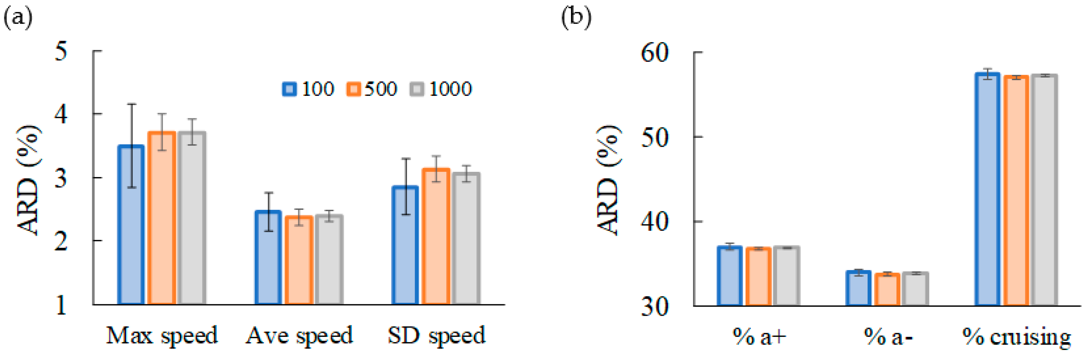
A major complication of this evaluation process is that the MT and MCMC methods produce different results every time they are used. To overcome this complication, we repeated the DC construction process several times and observed the average of the RDi obtained (ARDi). Figure 4a shows, as an example, the ARDi obtained for the speed related CPs after 100, 500, and 1000 iterations of applying the MT method. Similarly, Figure 4b shows the ARDi obtained for the CPs related to the percentage of time in different modes of operation after 100, 500, and 1000 iterations of applying the MCMC method. Both figures also show the confidence interval of variation of the ARDi.

Figure 4a,b show that after 500 iterations the ARDi and their confidence intervals remain constant. Pairwise hypothesis tests on the difference of means and the difference of variances confirmed this observation with a significance value of α = 0.05 for all ARDi. Thus, from this point on we will only report ARDi after 500 iterations. The comparison of the FB, MT and MCMC methods of constructing DCs was complemented with a dispersion analysis of the RDi. We observed the variation of the RDi during the first 500 iterations. Some of the RDi exhibited an asymmetric distribution. Thus, we decided to use the inter-quartile range (IQR) as a metric for dispersion and to present the results in terms of whiskers and boxes plots.

3. Results and Discussion

Initially, we used the data from the 46 trips sampled in each region and obtained the average values for the 23 CPs that describe the respective driving pattern, fuel consumption and emission of pollutants. Table 4 shows the results obtained.

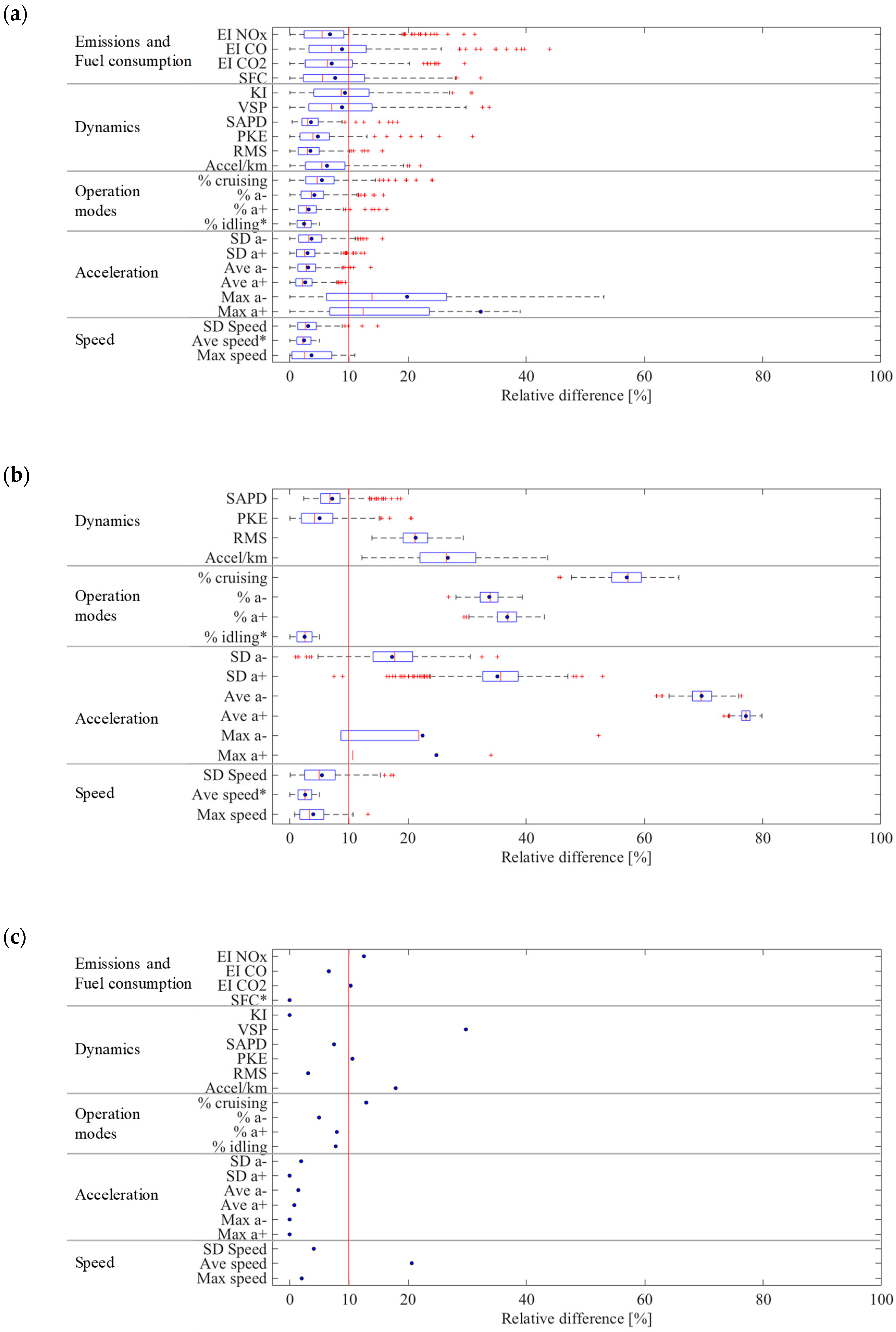
Then, we evaluated the ability of the three methods of producing DCs that represent the observed driving patterns. For the case of the general region, Figure 5a,b show the ARDi and the interquartile range of the RDi exhibited by the DCs obtained by the MT and MCMC methods, respectively, after repeating the application of each method 500 times. Figure 5c shows the same information for the case of the FB method. As mentioned before in this last case, results are the same every time the method is applied and therefore ARDi = RDi for all CPs. In Figure 5a,b, the ARDi are shown as blue dots, the IQRi by boxes, and the outliers by red “+” signs. The CPs used by each method as criteria for the construction of the DC are marked with (*).

A low ARDi (<10%) indicates that the method produced DCs that represent the driving pattern. The potential range of variation of the ARDi is from zero to infinity and therefore ARDi <10% indicates a high level of similitude. Table 4 presents the values of ARDi obtained for the 23 CPs. In this table, the ARDi below 10% are highlighted in green.

Since the set of CPs that describes a driving pattern is still undefined, the method´s ability of producing DCs that capture the local driving pattern is judged as the number of CPs where the ARDi < 10%. However, in this evaluation it is important to:

• Do not include the CPs used as the assessment criteria by the method under consideration to construct the DC because those CPs by design should be smaller than 5%.
• Consider as an independent case the SAPD due to the high relevance of this metric for some researchers and because its range of variations is from 0 to 200%.

For the general region, Table 4 and Figure 5a show that the FB method had 14 out of 19 CPs with ARDi < 10%, while the MT had 15 out of 17, and the MCMC only had four out of 15 CPs under this threshold.

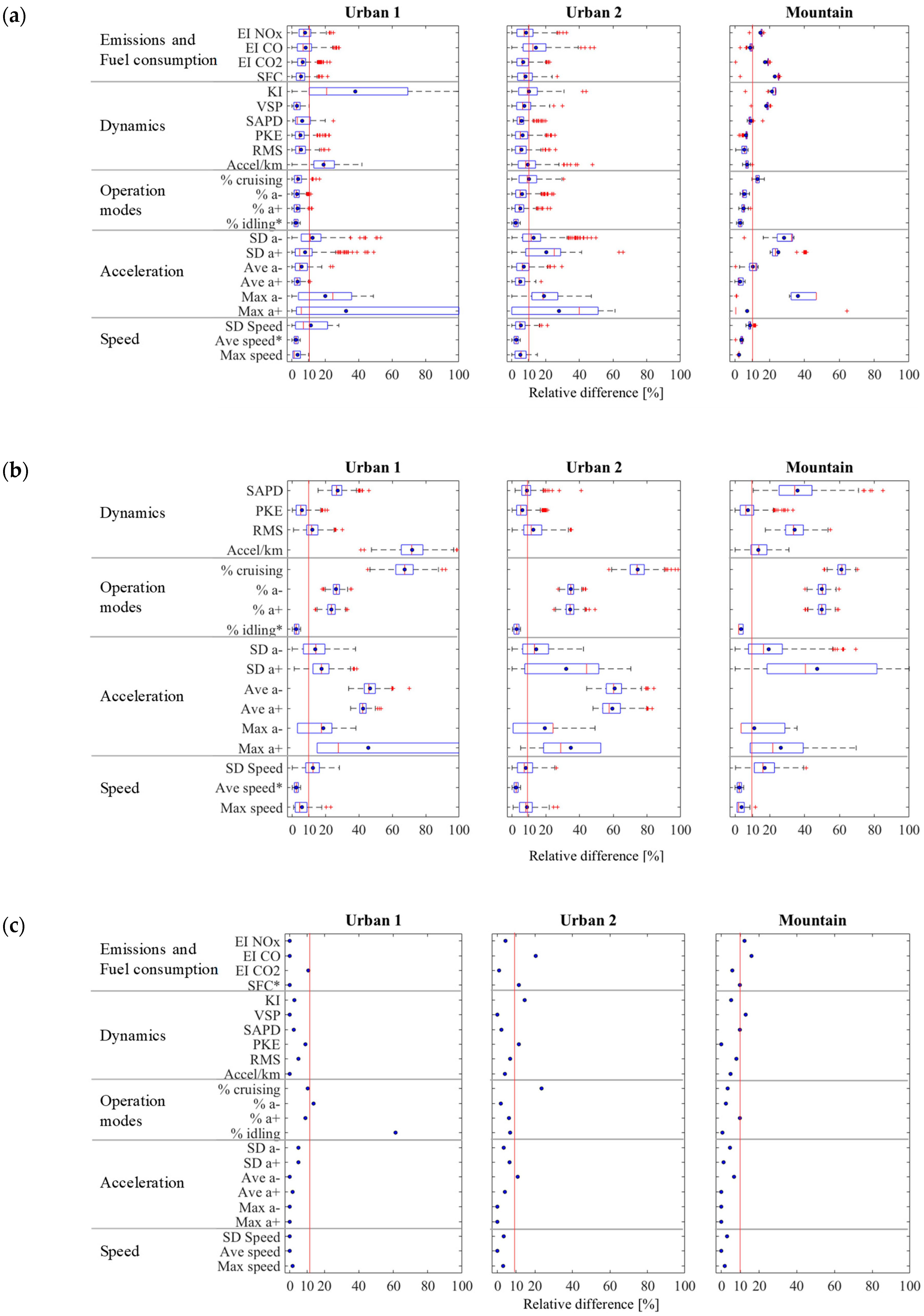
The same analysis was repeated for the case of the Mountain, Urban 1 and Urban 2 regions. Figure 6 shows that the results obtained for these three regions are similar to the results observed for the general region. Table 4 quantifies, in terms of ARDi, the performance of each method in the four regions considered in this study. Considering all the regions, the FB method showed 83% of the ARDi under 10%, while the MT showed 69% and the MCMC 20%, excluding the CPs used as assessment criteria. The average of the ARDi of the 19 CPs in the four regions was 5.8%, 10.1% and 34.9% in the FB, MT and MCMC methods, respectively.

On average over the four regions, the FB method constructed DCs with RDi smaller than 19.1%. The maximum RDi were observed for the percentage of idling time in the Urban 1 region and VSP in the General region that reached an RDi of 61.3% and 29.8%, respectively. The best performance of the FB method was observed in the mountain region where all RDi were below 16%. The FB method showed the most stable performance among the three methods in the four regions considered in this study.

The MT method (Figure 5a) produced DCs that represent well all CPs. Kinetic energy intensity and max des-acceleration were the CPs that showed the smallest agreement with ARDi of up to 38.1% and 36.1%, respectively. Compared to the general region, the MT method deteriorated its performance for the case of the region with highly congested traffic (Urban 1), where the CP associated to the kinetic energy intensity showed an ARDi of 38.1% with a large dispersion (RDi of up to 59%). Its performance worsens for the case of the mountain region where only 10 out of 17 CPs were below the 10% threshold for the ARDi.

The MCMC method showed the worst performance in producing DCs that represent local DC. It showed the smallest numbers of ARDi below the 10% threshold and the maximum range of variation of the RDi. The CPs with the largest ARDi were the number of accelerations per kilometer and the average positive acceleration reached ARDi of 163.8% (in the Urban 1 region) and 141.3% (in the mountain region), respectively, and with outliers for the corresponding RDi larger than 100% (not shown in Figure 5b). We also expected that this method produced DCs with the SAPD close to the SAPD of the driving pattern observed in each region, in consideration to its approach of constructing DCs. However, its performance was worse than the other two methods in this metric. On average over the four regions, it showed an ARDi of 19.7% vs an ARDi of 5.5% for the FB method and 6.2 for the MT method.

Previous results demonstrate the outstanding performance of the FB and MT methods producing DCs that represent the observed local driving patterns. Next, we will describe their performance reproducing fuel consumption and emissions of pollutants. By design, the FB method reproduced fuel consumption in all regions (RDi < 11% and on average 5.3%). Figure 5c, Figure 6c and Table 4 show that this method reproduced the CO, CO₂ and NO_x emissions with an RDi < 20%. The average RDi was 8.3%. This performance was followed closely by the MT method. On average, the MT method produced DCs that reproduced fuel consumption with an average ARDi of 11.1% and an average ARDi of 9.6% for the CO, CO₂ and NO_x emissions, in the four regions considered in this study.

As described before, the methodology used in this work does not allow to evaluate the performance of the MCMC method reproducing fuel consumption nor emission from the vehicles.

Previous results demonstrate that the FB method showed the best performance obtaining DCs that represent the driving patterns, the fuel consumption and emissions from the vehicles in the four regions considered in this study. Previous results also confirm that by using local DC instead of the type-approval DC, the differences between the fuel consumption and emissions from vehicles reported by manufactures and those observed in the normal use of the vehicles can be reduced substantially (<11% depending on the method used for constructing the local DC).

4. Conclusions

We hypothesized that the incorrect representation of the local driving patterns contained in the type-approval driving cycles used by manufacturers to report fuel consumption and emissions from vehicles, is one of the major sources of the differences observed between those values and the observed in the normal use of the vehicles. Thus, there is a need for local driving cycles (DCs) that truly represent local driving patterns and that could be used during the type-approval tests. However, there is not a unified method to construct those local DC. As an intermediate step, this work compared three common methods of constructing local DCs in their ability of producing DCs that: (i) represent the local driving patterns and (ii) reproduce the fuel consumption and emissions exhibited by the vehicles in that region. The methods studied were the Micro-Trips (MT), the Markov Chains-Monte Carlo (MCMC) and the Fuel-Based (FB).

To that end, we implemented those methods in four regions with different topographies, different altitudes, and featuring well-maintained roads with different Level of Services (LoS). We monitored during a prolonged period of time (~8 months) the operation of a fleet of 15 busses with the same emission control technology and with similar maintenance conditions in order to eliminate the effects of their variations in our results. We measured simultaneously fuel consumption, CO, CO₂ and NO_x emissions, speed, and location at 1 Hz.

Driving patterns and DCs can be described by characteristic parameters (CPs) such as mean speed, mean positive acceleration, among others. Hence, a DC represents a local driving pattern of a given region when its CPs are equal to the CPs that describe the driving pattern in that region. The level of similarity is measured by the relative differences among them. Since the MT and the MCMC are repeatable but no reproducible, we repeated the implementation of those methods up to 1000 times and reported the average relative differences (ARDi) of the obtained CPs.

Results demonstrated that the FB method showed the best performance obtaining DC that represent the driving patterns, the fuel consumption and emissions from the vehicles in the four regions considered in this study, followed closely by the MT method. The MCMC method has difficulties producing representative DCs. In all regions, the FB method exhibited 83% of the CPs with ARDi under 10%, while the MT and MCMC presented 69% and 20%, respectively. By design, the FB method reproduced fuel consumption in all regions (ARDi ~ 5.3%). Furthermore, this method also reproduced the CO, CO₂ and NO_x emissions with ARDi of 8.3%. This performance was followed closely by the MT method. On average, the MT method produced DCs that reproduced fuel consumption with an ARDi of 11.1% and of 9.6% for the CO, CO₂ and NO_x emissions.

Previous results also confirm that by using local DC instead of the type-approval DC, the differences between the fuel consumption and emissions from vehicles reported by manufactures and the observed in the normal use of the vehicles can be reduced substantially (<11% depending on the method used for constructing the local DC).

Besides providing a methodology to assess the representativeness of driving cycles and the performance of the methods to construct them, this works contributes suggesting alternatives to strengthen the MT method and a procedure to test the correct implementation of any method to construct driving cycles. Our work can also be used to identify the minimum set of CPs that fully describe driving patterns, and the design of a method to construct driving cycles for mountain regions. However further work is required to extend the scope of our conclusions to several vehicle technologies and to identify alternatives of implementing the resulting DC in chassis dynamometers.

References

- Tietge, U.; Mock, P.; Franco, V.; Zacharof, N. From laboratory to road: Modeling the divergence between official and real-world fuel consumption and CO2 emission values in the German passenger car market for the years 2001–2014. Energy Policy 2017, 103, 212–222. [Google Scholar] [CrossRef]
- Ntziachristos, L.; Mellios, G.; Tsokolis, D.; Keller, M.; Hausberger, S.; Ligterink, N.E.; Dilara, P. In-use vs. type-approval fuel consumption of current passenger cars in Europe. Energy Policy 2014, 67, 403–411. [Google Scholar] [CrossRef]
- Duarte, G.O.; Gonçalves, G.A.; Farias, T.L. Analysis of fuel consumption and pollutant emissions of regulated and alternative driving cycles based on real-world measurements. Transp. Res. Part D 2016, 44, 43–54. [Google Scholar] [CrossRef]
- Gong, Q.; Midlam-mohler, S.; Marano, V.; Rizzoni, G. An Iterative Markov Chain Approach for Generating Vehicle Driving Cycles. Int. J. Engines 2017, 4, 1035–1045. [Google Scholar] [CrossRef]
- Ligterink, N.E.; Eijk, A.R.A. Update Analysis of Real-World Fuel Consumption of Business Passenger Cars Based on Travelcard Nederland Fuelpass Data; TNO: Delft, The Netherlands, 2014; p. 25. [Google Scholar] [CrossRef]
- Tietge, U.; Mock, P.; Franco, V.; Zacharof, N. From Laboratory to Road A 2017 Update of official and “Real-World” Fuel Consumption and CO2 Values for Passenger Cars in Europe. Energy Policy 2017, 103, 212–222. [Google Scholar] [CrossRef]
- Fontaras, G.; Zacharof, N.G.; Ciuffo, B. Fuel consumption and CO2 emissions from passenger cars in Europe –Laboratory versus real-world emissions. Prog. Energy Combust. Sci. 2017, 60, 97–131. [Google Scholar] [CrossRef]
- Ministre de L’Environnement de L’Énergie et de la mer. Contrôles des Émissions de Polluants Atmosphériques et de CO2; Ministre de L’Environnement de L’Énergie et de la mer: Paris, France, 2016.
- Tong, H.Y.; Hung, W.T. A framework for developing driving cycles with on-road driving data. Transp. Rev. 2010, 30, 589–615. [Google Scholar] [CrossRef]
- Giakoumis, E.G. Driving and Engine Cycles; Springer International Publishing: Cham, Switzerland, 2017. [Google Scholar]
- Huang, D.; Xie, H.; Ma, H.; Sun, Q. Driving cycle prediction model based on bus route features. Transp. Res. Part D 2017, 54, 99–113. [Google Scholar] [CrossRef]
- Shi, S.; Lin, N.; Zhang, Y.; Cheng, J.; Huang, C.; Liu, L.; Lu, B. Research on Markov property analysis of driving cycles and its application. Transp. Res. Part D 2016, 47, 171–181. [Google Scholar] [CrossRef]
- Tutuianu, M.; Bonnel, P.; Ciuffo, B.; Haniu, T.; Ichikawa, N.; Marotta, A.; Pavlovic, J. Development of the World-wide harmonized Light duty Test Cycle (WLTC) and a possible pathway for its introduction in the European legislation. Transp. Res. Part D Transp. Environ. 2015, 40, 61–75. [Google Scholar] [CrossRef]
- Huertas, J.; Giraldo, M.; Quirama, L.; Díaz, J. Driving Cycles Based on Fuel Consumption. Energies 2018, 11, 3064. [Google Scholar] [CrossRef]
- Hung, W.T.; Tong, H.Y.; Lee, C.P.; Ha, K.; Pao, L.Y. Development of a practical driving cycle construction methodology: A case study in Hong Kong. Transp. Res. Part D Transp. Environ. 2007, 12, 115–128. [Google Scholar] [CrossRef]
- Arun, N.H.; Mahesh, S.; Ramadurai, G.; Shiva Nagendra, S.M. Development of driving cycles for passenger cars and motorcycles in Chennai, India. Sustain. Cities Soc. 2017, 32, 508–512. [Google Scholar] [CrossRef]
- Brady, J.; O’Mahony, M. Development of a driving cycle to evaluate the energy economy of electric vehicles in urban areas. Appl. Energy 2016, 177, 165–178. [Google Scholar] [CrossRef]
- Tzeng, G.-H.; June-Jye, C. Developing a Taipei Motorcycle Driving Cycle for Emissions and Fuel Economy. Transp. Res. Part D 1998, 3, 19–27. [Google Scholar] [CrossRef]
- Lin, J.; Niemeier, D.A. An exploratory analysis comparing a stochastic driving cycle to California’s regulatory cycle. Atmos. Environ. 2002, 36, 5759–5770. [Google Scholar] [CrossRef]
- Huertas, J.I.; Díaz, J.; Cordero, D.; Cedillo, K. A new methodology to determine typical driving cycles for the design of vehicles power trains. Int. J. Interact. Des. Manuf. 2018, 12, 319–326. [Google Scholar] [CrossRef]
- HCM. Highway Capacity Manual 2010; Transportation Research Board: Washington, DC, USA, 2010; ISBN 0738-6826. [Google Scholar]
- Pīrs, V.; Jesko, Ž.; Lāceklis-Bertmanis, J. Determination methods of fuel consumption in laboratory conditions. Eng. Rural Dev. 2008, 1, 154–159. [Google Scholar]
- SAE-J1321. Fuel Consumption Test Procedure-Type II. SAE Int. 2012, 50. [Google Scholar] [CrossRef]
- USEPA. Determination of PEMS Measurement Allowances for Gaseous Emissions Regulated under the Heavy-Duty Diesel Engine In-Use Testing Program; USEPA: Washington, DC, USA, 2008.
- Galgamuwa, U.; Perera, L.; Bandara, S. Developing a General Methodology for Driving Cycle Construction: Comparison of Various Established Driving Cycles in the World to Propose a General Approach. J. Transp. Technol. 2015, 5, 191–203. [Google Scholar] [CrossRef]
- Liu, J.; Wang, X.; Khattak, A. Customizing driving cycles to support vehicle purchase and use decisions: Fuel economy estimation for alternative fuel vehicle users. Transp. Res. Part C Emerg. Technol. 2016, 67, 280–298. [Google Scholar] [CrossRef]
- Zhang, X.; Zhao, D.J.; Shen, J.M. A synthesis of methodologies and practices for developing driving cycles. Energy Procedia 2011, 16, 1868–1873. [Google Scholar] [CrossRef]
Figure 1.
Relative differences of the values reported by manufacturers with respect to the real fuel consumption or real CO2 emissions as function of the vehicles’ model year. Sources: (a) [1], (b) [2], (c) [3], (d) [4], (e) [5], (f) [6], (g) [7], and (h) [8]. Dotted lines shows the tendency obtained from the data of reference (f) which are shown as red dots. References e-h include diesel and gasoline.
Figure 2.
Illustration of the methodology followed to compare three alternatives to construct representative driving cycles.
Figure 3.
Illustration of the test used to verify the correct implementation of the methods to construct DCs. Artificial trips used (left side) and DCs (right side) obtained by (a) the MCMC and (b) the MT methods.
Figure 4.
ARDi and their confidence intervals for some CPs with different number of runs. (a) Speed related CPs when applied MT. (b) Operation mode related CPs when applied MCMC.
Figure 5.
Boxplots of the relative differences (RDi) of the CPs that describe the DCs obtained by the (a) MT, (b) MCMC, and (c) FB methods in the general region after 500 iterations. The ARDi are shown as blue dots, the IQRi by boxes, and the outliers by red “+” signs. The CPs used by each method as criteria for the construction of the DC are marked with (*).
Figure 6.
Boxplots of the relative differences (RDi) of the CPs that describe the DCs obtained by the (a) MT, (b) MCMC, and (c) FB methods in the Urban 1, Urban 2 and Mountain regions after 500 iterations. The ARDi are shown as blue dots, the IQRi by boxes, and the outliers by red “+” signs. The CPs used by each method as the criteria for the construction of the DC are marked with (*).