Diesel Engine Valve Clearance Fault Diagnosis Based on Improved Variational Mode Decomposition and Bispectrum


1
Department of Mechanics, Tianjin University, Tianjin 300354, China
2
Department of Industrial Technology, California State University, Fresno, CA 93740, USA
3
Tianjin Key Laboratory of Nonlinear Dynamics and Control, Tianjin 300354, China
4
National Demonstration Center for Experimental Mechanics Education (Tianjin University), Tianjin 300354, China
*
Authors to whom correspondence should be addressed.
Energies 2019, 12(4), 661; https://doi.org/10.3390/en12040661
Submission received: 7 January 2019
/
Revised: 14 February 2019
/
Accepted: 17 February 2019
/
Published: 19 February 2019
Abstract
:The evaluation and fault diagnosis of a diesel engine’s health conditions without disassembly are very important for diesel engine safe operation. Currently, the research on fault diagnosis has focused on the time domain or frequency domain processing of vibration signals. However, early fault signals are mostly weak energy signals, and the fault information cannot be completely extracted by time domain and frequency domain analysis. Thus, in this article, a novel fault diagnosis method of diesel engine valve clearance using the improved variational mode decomposition (VMD) and bispectrum algorithm is proposed. First, the experimental study was designed to obtain fault vibration signals. The improved VMD method by choosing the optimal decomposition layers is applied to denoise vibration signals. Then the bispectrum analysis of the reconstructed signal after VMD decomposition is carried out. The results show that bispectrum image under different working conditions exhibits obviously different characteristics respectively. At last, the diagonal projection method proposed in this paper was used to process the bispectrum image, and the fourth order cumulant is calculated. The calculation results show that three states of the valve clearance are successfully distinguished.
1. Introduction
Abnormal valve clearance is one of the most common faults in the valve mechanism of a diesel engine [1]. It can cause valve switch timing changes, affect the quality of air exchange in the cylinder, cause combustion deterioration, and affect the emission and economy of the diesel engine. It is of great significance for condition monitoring and fault diagnosis of diesel engine valve clearance. The vibration signal of diesel engine cylinder head contains much information about working state and fault characteristics. Extracting proper characteristic parameters from the vibration signal can effectively identify the working state and related faults of a diesel engine [2,3,4].
Due to the complex structure and vibration sources of diesel engine, the vibration signal of diesel engine contains much noise. In addition, in the early stage of the engine fault, the vibration characteristic energy which indicates the fault information is weak and cannot be extracted directly. Therefore, the vibration signals need to be further processed to identify the fault characteristics.
Traditional signal processing techniques used in mechanical fault diagnosis can be divided into two categories: time domain analysis and frequency domain analysis. Time domain analysis mainly includes probability analysis method, the time domain synchronous averaging method and the correlation function diagnosis method. Fault information is extracted by calculating the characteristic quantity of time domain signals, such as vibration amplitude, root mean square value, skewness, kurtosis, etc. Frequency domain analysis is mainly based on Fourier transform, including spectrum analysis, power spectrum analysis and envelope analysis etc.
Traditional signal processing technology is mature in theory and practical application. However, due to its own limitation, it is only suitable for analyzing stationary signals. When engine fault occurs, the fault information is usually very weak. The fault features contain a lot of nonstationary nonlinear information, which seriously affects the accuracy of fault feature extraction [5]. That means the fault information in vibration signals of diesel engine are not be completely reflected by time-domain waveform or frequency spectral examination.
In recent years, various signal processing algorithms have been used in fault diagnosis fields, such as wavelet transform (WT), wavelet packet transform (WPT), empirical mode decomposition (EMD), local mean decomposition (LMD) and variational mode decomposition (VMD) [6,7,8,9,10]. The WT and WPT methods were found to be more suitable for nonstationary signal analysis than the FFT as a result of its high time-frequency resolution. But both of them cannot extract nonlinear relationships within the signal clearly. The EMD algorithm is an effective method for analyzing nonsteady and nonlinear signals. Compared with wavelet transform, the EMD method can decompose the original signal into a series of intrinsic mode functions (IMF) adaptively according to the local time scale characteristics of the signal without selecting the wavelet base function. But EMD still has its drawbacks, such as the end effects, and the mode mixing problem. The EEMD method can improve the disadvantage of EMD [11], but the low computational efficiency of EEMD limits its application for online detection. VMD method is a new adaptive signal decomposition method proposed by Dragomiretskiy et al [12]. This method uses iterative search for the optimal solution of the variational model to determine the bandwidth and central frequency of each decompose component, so that the signal can be decomposed adaptively. Compared with the recursive filter mode of the EMD method, the essence of VMD is multiple adaptive Wiener filter groups, which shows more robustness [13,14,15].
Although showing a great advantage over other algorithms, the selection of decomposition layers K of VMD algorithm has no accepted method as of yet. In this paper, a decomposition layer selection method based on component center frequency fluctuation is proposed and applied to denoising the vibration signals of diesel engine. This method can make the frequency components of the decomposition results clearer, and the main components of the original signal are fully retained.
As the structure of a diesel engine is complex, all kinds of excitations are reflected in the vibration of the engine surface by the corresponding transfer and coupling, which makes the measured engine vibration signal very complex. At the same time, most of the abnormal signals at the beginning of the fault are weak energy signals, which are often submerged in the strong background noise. However, noise signals often have strong Gauss characteristics, but the fault information often has a non-Gauss characteristic [16]. Higher order spectra (HOS) analysis is a mathematical tool to describe the high order statistical characteristics of random variables. This theoretical approach shows great performance for extracting nonlinear, non-Gauss and nonstationary characteristics of signals. Bispectrum is the lowest and most widely used high-order spectrum method; it can suppress the Gauss component in the signal and analyze the phase coupling relationship between the frequency components of the signal. The bispectrum diagram can reflect the distribution form and intensity of non-Gauss component of vibration signal in dual-frequency domain. For the above factors, the bispectrum analysis is widely used in the field of mechanical fault diagnosis [17,18,19,20]. Usually, bispectrum image is sliced diagonally and analyzed to evaluate fault severity. However, diagonal slicing will lose much information of the bispectrum image. In this article, the diagonal projection processing method of bispectrum is proposed. This method can extract fault features precisely.
The improved VMD method can decompose a complex signal into several IMF components from high to low frequency and can avoid mode mixing. Therefore, the engine fault characteristics hidden in the vibration signals can be decomposed into a specific IMF component. The bispectrum analysis to the reconstructed signal after VMD decomposition can further acquire the nonlinear and non-Gauss characteristics of fault features. This paper presents a new approach on the basis of improved VMD and bispectrumis proposed for the fault diagnosis of diesel engine.
2. Methodology
2.1. VMD
2.1.1. The Theory of the VMD Algorithm
The function of the VMD algorithm is to decompose a signal f into several discrete modal components uk. For each modal component of uk, the central frequency is determined by the number of decomposition layers, and almost every modal component is close to the central frequency. That is, each modal has a specific sparsity and is able to reconstruct the original signal. The steps of VMD decomposition are shown as follows [12]:
First, the bandwidth of modal components uk needs to be estimated. For each modal component, the Hilbert transform is used to process the signal to obtain the single side spectrum:
In this equation, Huk(t) is the single side spectrum, is the Dirac distribution, k is the number of modes, uk(t) denotes mode function and “*” is the convolution operation symbol. For the two functions and , the convolution operation is defined as: .
Then mixing the predicted center frequencies of the single-side spectrum, the analytic signal is obtained. The analytic signal of the modal function is as follows,
In this equation, Auk(t) is the analytic signal and ωk is the center frequency of each modal component.
After processing by Equation (2), the bandwidth can be obtained by the square of L2 norm, which is the Gauss smoothing of the demodulated signal. The constrained variational model is obtained as follows:
In the above equation, are the full modal components, are the central frequencies of modal components. is the sum of all modes.
There are many ways to solve this problem. For VMD, the quadratic penalty term and Lagrange multiplier λ are added into the VMD algorithm to obtain the unconstrained equation. The quadratic penalty can guarantee the accuracy of signal reconstruction under the Gauss noise interference. Lagrange multipliers guarantee the strictness of constraint conditions. By the combination of these two methods, the quadratic penalty term has a good convergence property under the finite weight, so that the quadratic penalty term will not be infinite because of the absence of noise. Based on this method, the augmented Lagrangian formula can be obtained as follows:
The minimum value in original Equation (3) now has been changed into a saddle point problem for the augmented Lagrangian formula (4). This problem can be solved by repeated local optimization of uk, ωk, and λ. The updated process is shown as follows:
First, initialize uk, ωk, λ, n as 0, then update uk as follows:
By overwriting Equation (5), we can get the minimization equation as follows:
Then update ωk:
And update λ:
Repeat the above steps until satisfied the iterative stop condition as follows:
Then the cycle will stop, K modal components are obtained.
2.1.2. Verification of VMD Algorithm
In order to verify the superiority of the VMD method compared with the EMD method, two algorithms are used respectively to analyze an analog signal in this paper.
The analog signal is composed by four different components: 50 Hz sinusoidal signal, 100 Hz sinusoidal signal, impulse signal and noise signal (to make the noise more similar to actual signals, we selected non-Gaussian noise). The analog signal and its components are shown in Figure 1.
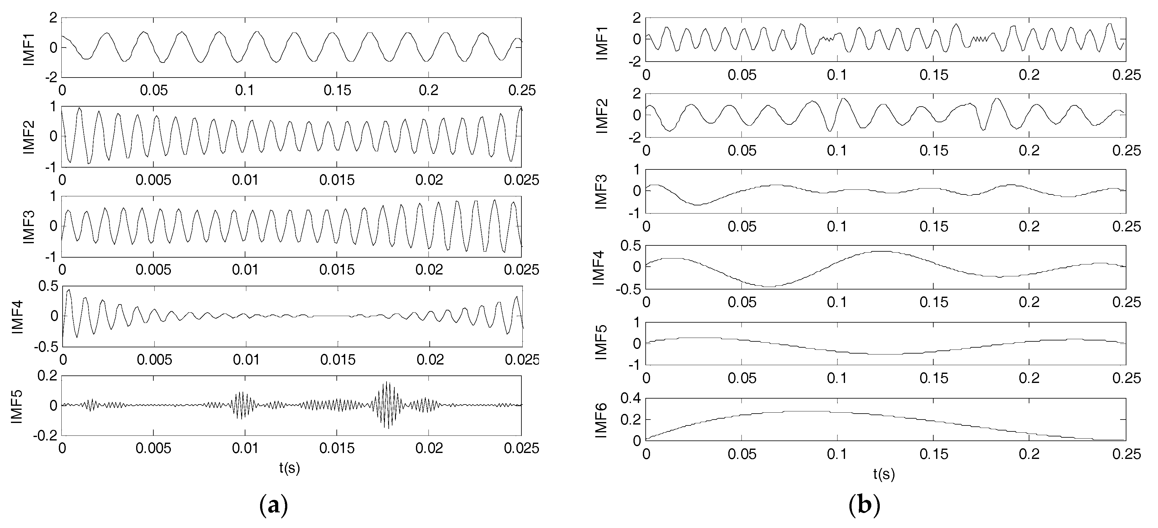
For the VMD algorithm, the number of decomposition layers was chosen as K = 5, according to the composition of the analog signal and the complexity of the noise signal. For EMD algorithm, the decomposition result is obtained automatically by convergence condition, and the final result of EMD decomposition is six layers. The results of VMD algorithm and EMD algorithm are shown in Figure 2.
From Figure 2a, it can be seen that VMD method can separate the 100 Hz sinusoidal signal, 50 Hz sinusoidal signal, and impulse signal from the original signal accurately. However, the EMD decomposition result shows obvious mode aliasing problem. The impulse signal and 100 Hz sinusoidal signal are all appeared in IMF1. The result shows that VMD algorithm has high accuracy.
2.2. Bispectrum
2.2.1. The Definition of Bispectrum
For the stationary vibration signal X(n), the bispectrum is defined as:
From this equation, it can be found that the bispectrum has two frequency variables ω1, ω2, the bispectrum amplitude of X(n) at (ω1, ω2) is equal to the product of the spectrum amplitude at ω1, ω2 and (ω1 + ω2)/2. Bispectrum has amplitude information and phase information, which can describe signal nonlinearity and non-Gauss characteristics. When the mechanical system is broken or the state changes, the nonlinear characteristic of the system will change. The quadratic phase coupling is a common nonlinear phenomenon, which means two frequency components in the signal interact with each other, and the corresponding phase relationship is called the quadratic phase coupling. The quadratic phase coupling information can be extracted by using bispectrum to describe the quadratic phase coupling quantitatively.
2.2.2. Bispectrum Calculation
There are many different methods that can calculate the bispectrum. The direct calculation method has higher accuracy, and its algorithm steps are shown as follows [21]:
(1) The test data X = [x1,x2,…,xm] are divided into Y segments of observation data and each segment contains M data samples.
(2) The mean value is removed from the observed data of each segment.
(3) Add the windows and calculate the discrete Fourier variation coefficients for each segment of data.
where = 0,1,…,M/2, i = 1,2,…,Y.
(4) The bispectrum by of the y-th order record is computed as:
where xi denotes the FFT of the y-th record.
(5) Finally, the average value of By is calculated as the result of bispectrum estimates.
2.2.3. Bispectrum Slice
Because bispectrum is a two-dimensional function, it is difficult to extract and analyze the image features compared with one-dimensional curve. In practical application, the signal feature is usually analyzed by bispectrum one-dimensional slice. The bispectrum one-dimensional slice is defined as one-dimensional Fourier transform of cumulant slice. For bispectrum Bx(ω1, ω2), fix any independent variables ω1 or ω2, the calculation result Bx(ω1, ω2) is one dimensional slice. When ω1 = ω2, the bispectrum diagonal slice can be obtained.
3. Engine Test Program and Experimental Data Acquisition
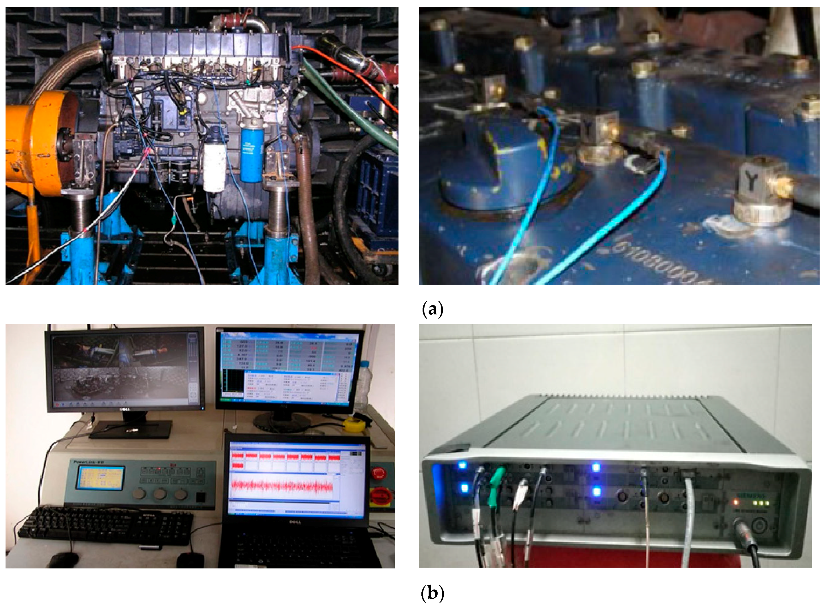
In this test, a six-cylinder inline diesel engine was used to generate the vibration signals. When the diesel engine is running, the pressure generated by the cylinder gas combustion and the impact of the inlet and exhaust valve movement act directly on the cylinder head and cause the cylinder head to vibrate. Therefore, the vibration signal of cylinder head contains abundant information, which is helpful for fault diagnosis. Three acceleration sensors were mounted on the cylinder head of cylinder 1- cylinder 3. The engine test condition was 2100 rpm—100% load. The vibration acceleration signals analyzed in this paper were collected by the acceleration sensor on cylinder 1. The data sampling frequency was 25,600 Hz. The fault parameters of the conditions are shown in Table 1. The test engine and the location of acceleration sensors are shown in Figure 3a, and the Dynamometer and LMS Scada III test system are shown in Figure 3b.
4. Results
4.1. Signal Denoising by Improved VMD
The change of valve clearance will directly result in the change of intake and exhaust valve mechanism and intake and exhaust state. The change of engine mechanical system will influence the characteristics of whole diesel engine. Thus, the vibration response will change. The valve clearance states can be categorized into three groups: the big valve clearance condition, normal valve clearance condition and small valve clearance condition. In order to further analyze the frequency components of cylinder head vibration signals under different valve clearance states, the power spectral density (PSD) analysis of the vibration signals under three working conditions was carried out.
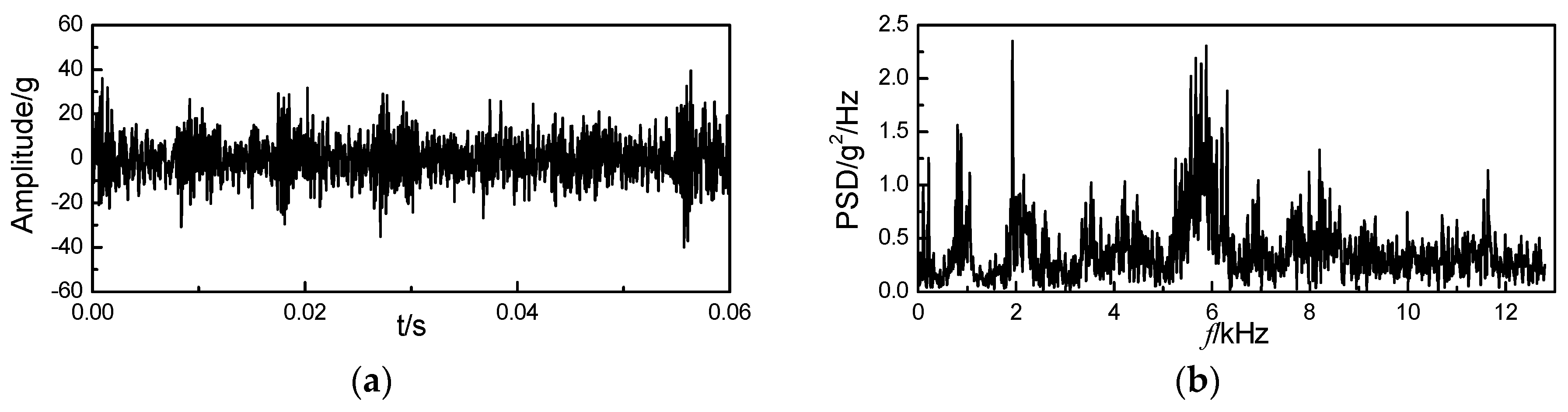
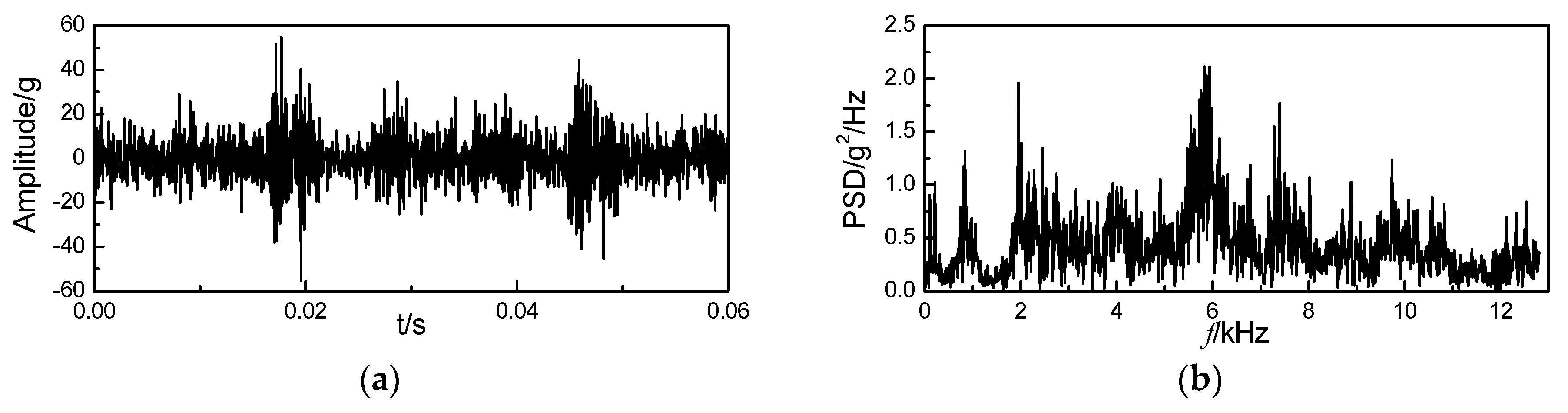
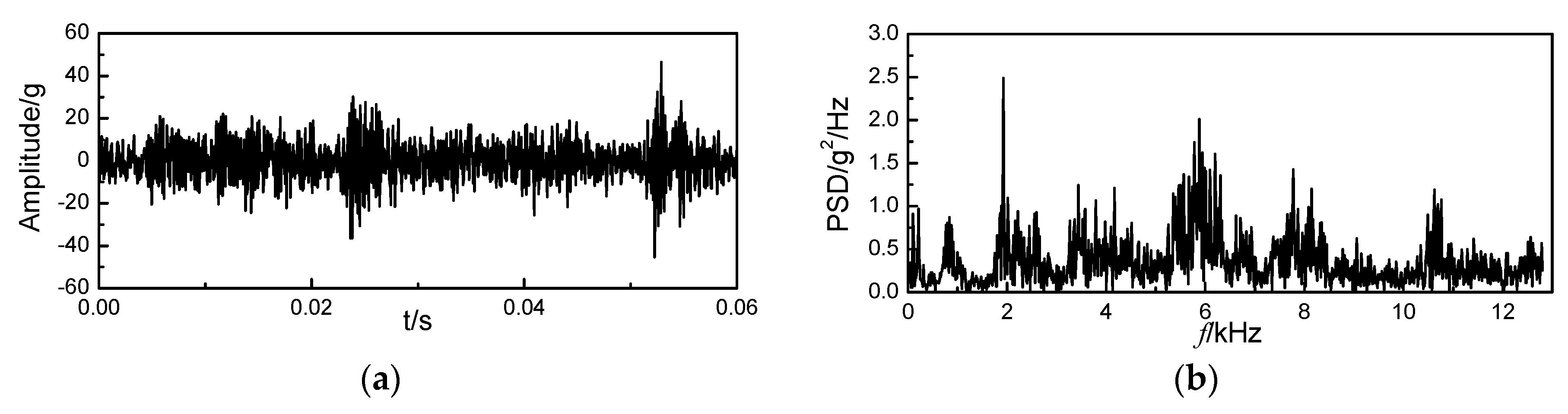
Figure 4a, Figure 5a and Figure 6a show the vibration curves under a big valve clearance condition, normal valve clearance condition and small valve clearance condition, respectively. PSD explains energy distribution of signal in the frequency domain. Figure 4b, Figure 5b and Figure 6b show the results of the vibration signal PSD estimations for big valve clearance condition, normal valve clearance condition and small valve clearance condition.
From Figure 4a, Figure 5a and Figure 6a, it can be found that the vibration signal of cylinder head under different valve clearance states are composed of a series of shock response signals according to certain time series. Though the time domain waveform of cylinder head vibration signals under different valve clearance states are different, we can’t find the variation rule of vibration signal in different valve clearance states directly from time domain waveform. And from Figure 4b, Figure 5b and Figure 6b, we can find that in all three valve-clearance states, the cylinder head vibration signals have peak values on both 2k Hz and 6k Hz. However, there are many noise components in the frequency domain, and the peak value of each frequency band is not prominent. So, the vibration signals need to be further processed.
Firstly, the vibration signals are decomposed by the VMD method. There are generally two methods for determining the number of decomposition layers in VMD algorithm. The first method is to select the best decomposition result by comparing the decomposition results under different decomposition layers. The second method is to determine the appropriate decomposition layers in advance through a certain prior knowledge. The second method is more efficient in practical calculation. If the appropriate decomposition layer is determined according to the prior knowledge, the higher accuracy can also be obtained. So, in this paper, the second method to determine the decomposition layer is used. According to the introduction of VMD algorithm above, the VMD algorithm is closely related to the central frequency of the component in the decomposition process. The frequency of the decomposition result is single or not is also an important index to evaluate the validity of the decomposition algorithm. Therefore, a decomposition layer selection method based on component central frequency fluctuation is proposed in this paper.
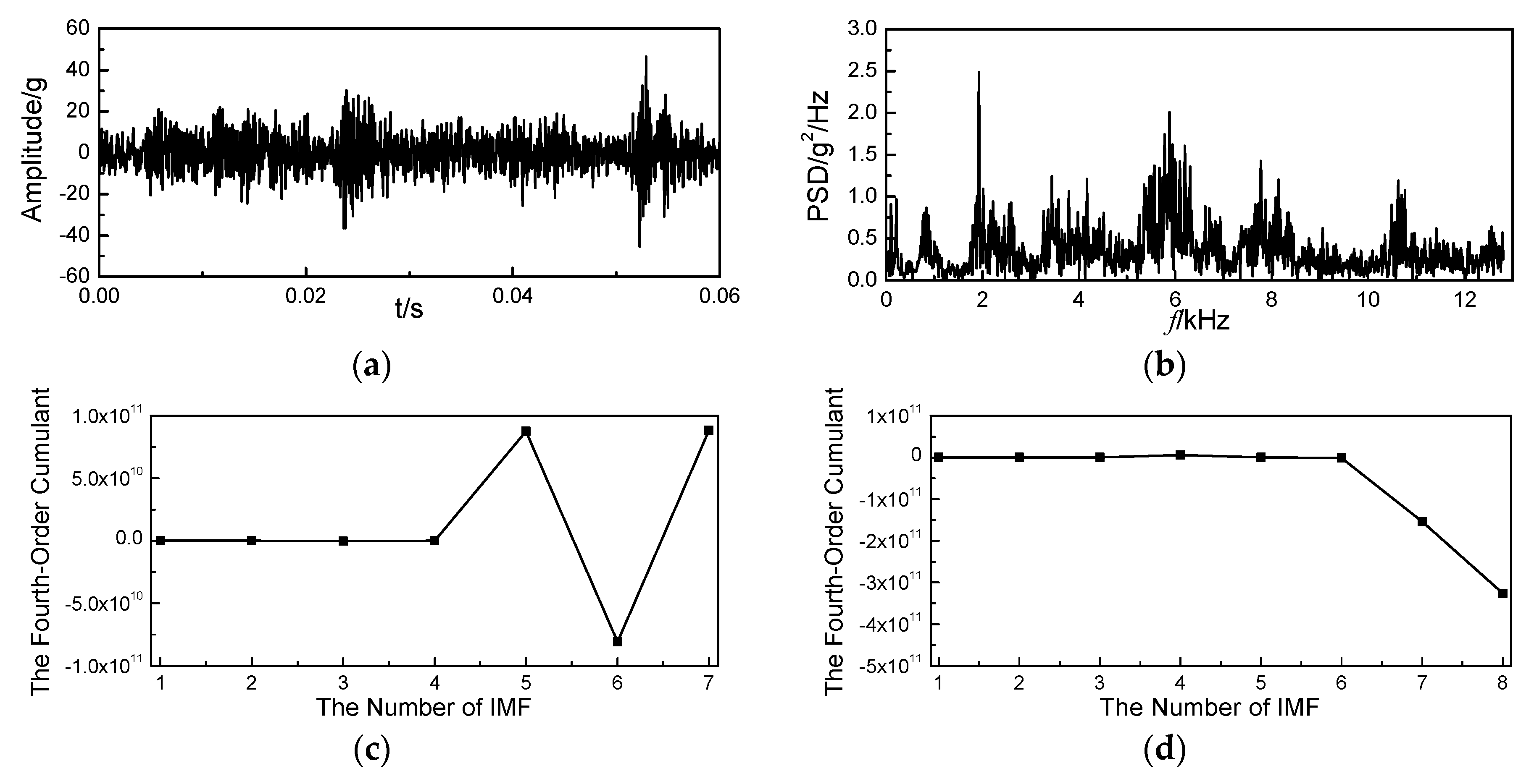
In order to determine the optimal number of decomposition layers, 80 segments of each signal are selected for analysis under three conditions: normal valve clearance, big valve clearance, and small valve clearance. In the analysis process, the 240-segment signal was decomposed into 5/6/7/8 layers by the VMD algorithm, respectively. According to previous experiments, the optimum decomposition level of engine vibration signal is generally within this range. After the decomposition, the central frequency of each order component under different decomposition layers is calculated. Then the fourth-order cumulant of central frequency of each order component was calculated to indicate the extent of its fluctuations (the fourth-order cumulant will increase with the enhancement of the signals’ non-Gauss property, so it can be used to characterize the fluctuation of the signal). The results are shown in Figure 7.
As can be seen from the above figures, the fluctuation of the whole states is the gentlest when K = 5 and K = 6. To further prove this point, the fourth-order cumulant of the central frequency of each order component at different K levels in Figure 7a–d above is calculated. The results are shown in Table 2 below:
As is shown in Table 2, the fluctuation of central frequency is the smallest when the decomposition layer K = 6, so it can be concluded that K = 6 is the best number of decomposition layers suitable for the current vibration signal decomposition. In particular, it can be seen from Figure 7a–d that, regardless of the value of K, the central frequency of the last order component in the decomposition results fluctuates greatly because the central frequency of last order component is near 10 kHz. It is generally believed that the vibration is very complicated due to the large number of vibration sources near this frequency, but comprehensive observation does not affect that K = 6 is the best number of decomposition layers.
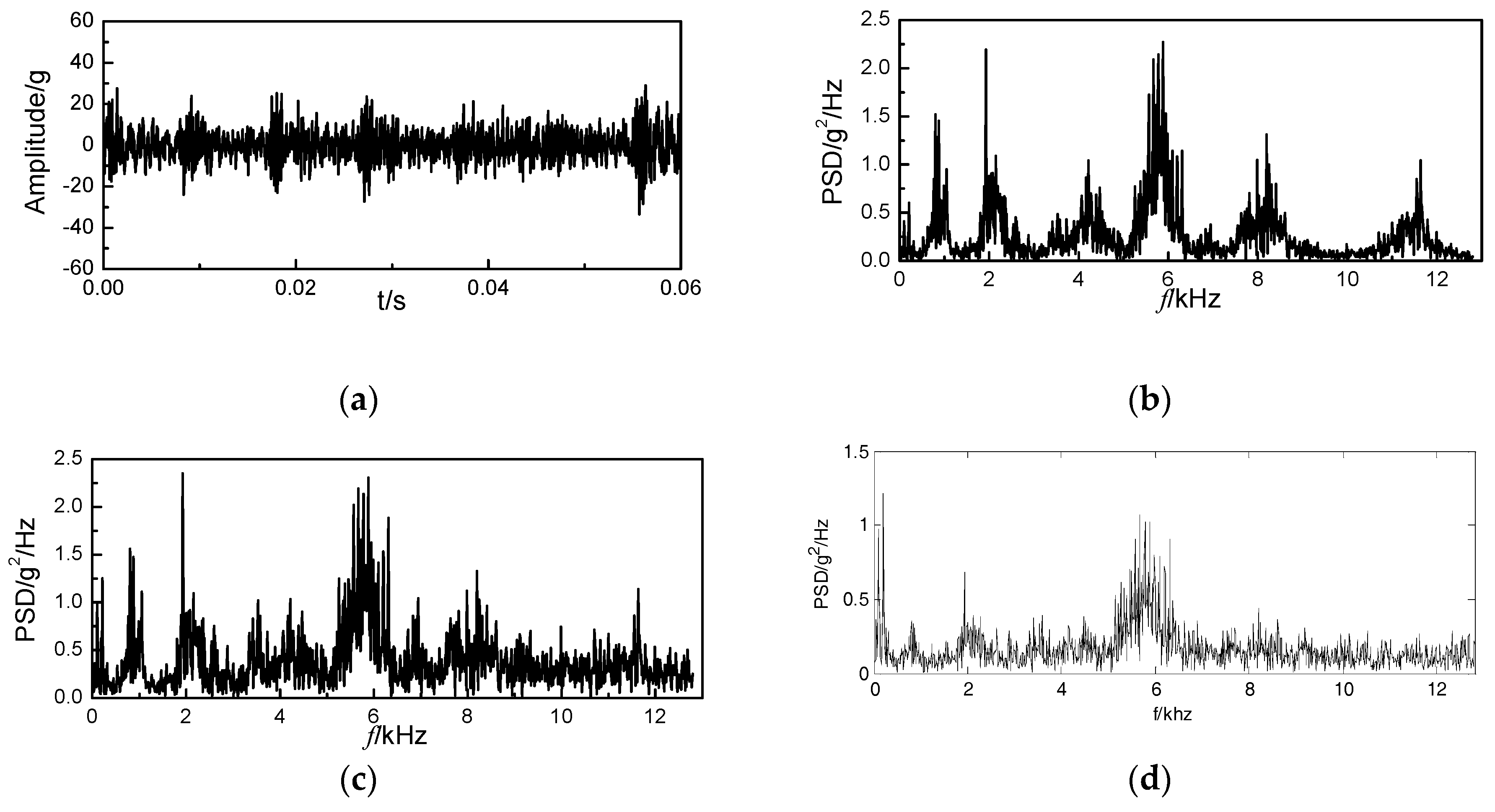
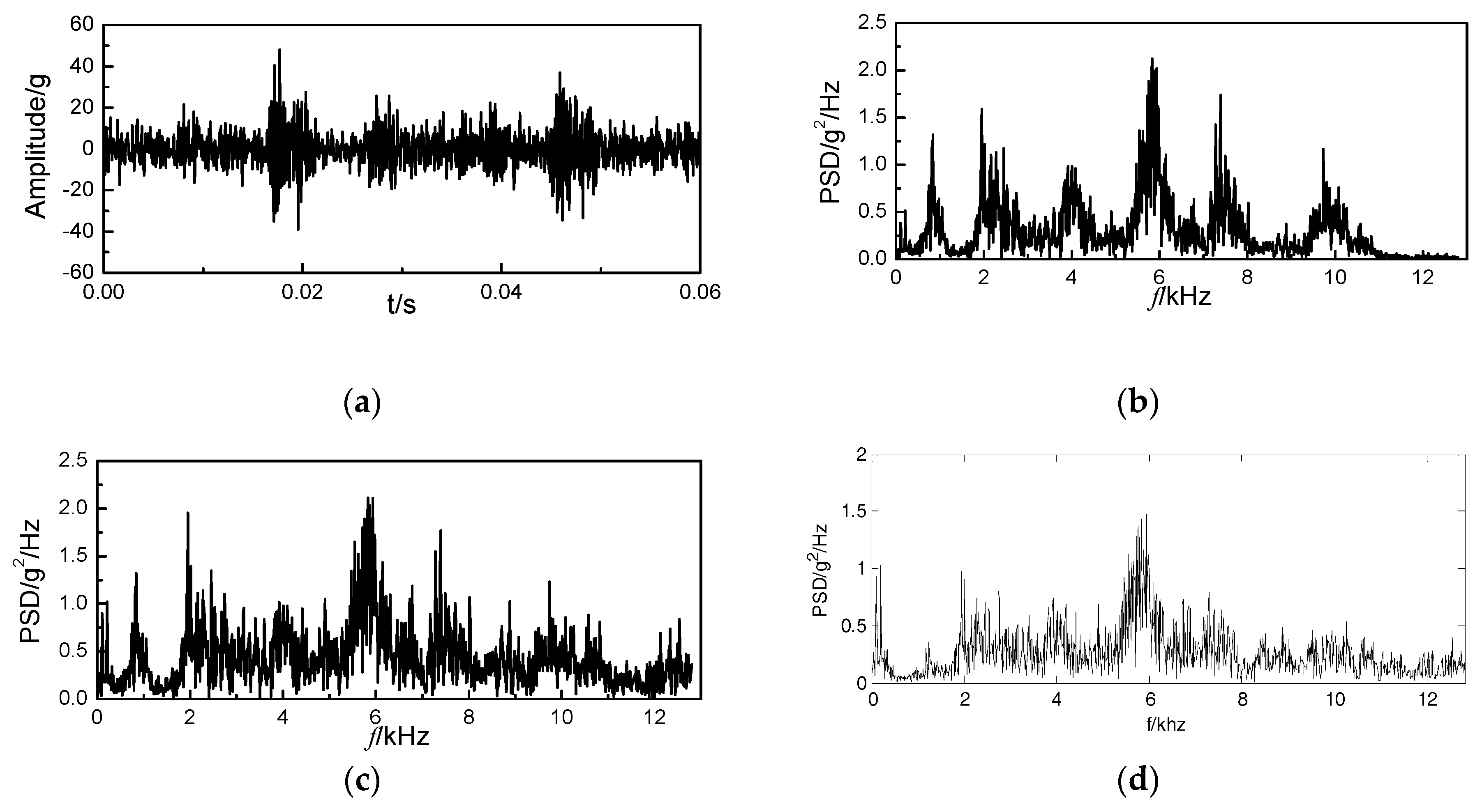
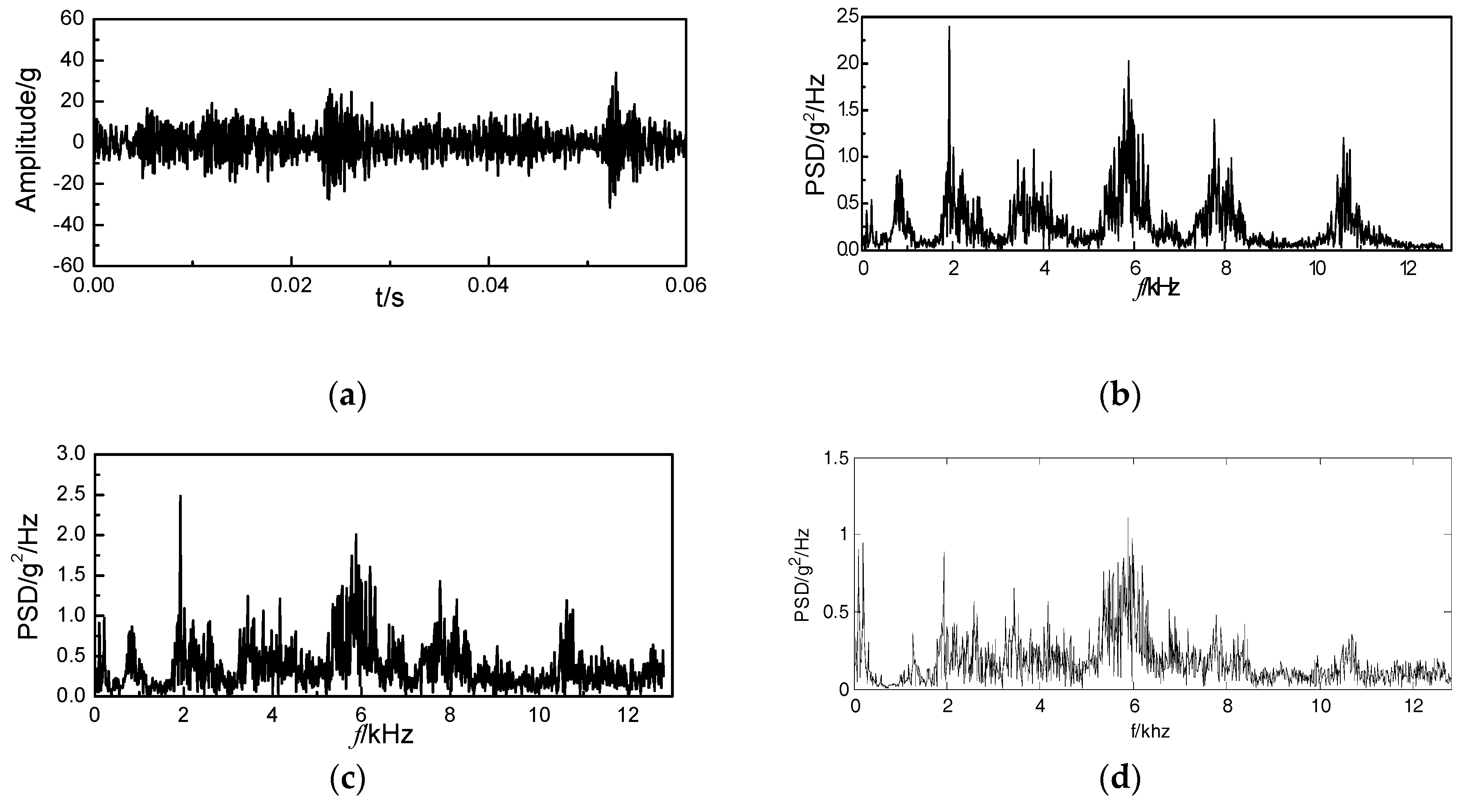
After determining the optimal number of VMD decomposition layers for the vibration signal of diesel engine, the VMD algorithm was used to process the original vibration signal. The specific process is to decompose and reconstruct a segment of signal using the VMD algorithm. After decomposing, the VMD results are reconstructed to a new signal for further processing. The reconstructed signals of the three conditions shown in Figure 4, Figure 5 and Figure 6 are shown in Figure 8a, Figure 9a and Figure 10a; the frequency domain curves are shown in Figure 8b, Figure 9b and Figure 10b. For comparison, the frequency domain curve of the original vibration signal is shown in Figure 8c, Figure 9c and Figure 10c. To verify the effectiveness of the improved method, a commonly used denoising method, the wavelet denoising method was used to analyze the vibration signals show in Figure 4a, Figure 5a and Figure 6a. Daubechies (db) wavelet is a type of wavelet function commonly employed in the field of fault diagnosis and signal processing [21], therefore, the db5 wavelet was used to denoise the vibration signal. After wavelet denoising, the PSD estimation was used to explain energy distribution of denoised signal in the frequency domain, the PSD results are shown in Figure 8c, Figure 9c and Figure 10c.
As can be seen from Figure 8, Figure 9 and Figure 10, compared to the frequency curve of original signal, the frequency components of the reconstructed signals are very clear, the noise components are minimal, and the information in each frequency band of original signals are preserved to the maximum extent. In contrast, as is shown Figure 8d, Figure 9d and Figure 10d, the wavelet denoising method can also achieve good denoising effect. But from the frequency waveforms, it can be found that the wavelet denoising method mainly retains the obvious peak values of 2 kHz and 6 kHz in the original signal, while the peak values of other frequency bands are basically removed. That may cause the denoised signal to lose part of fault information. To better illustrate this problem, the average energy EAverage is defined by the following equation:
In this equation, x(i) is the i-th data point of the signal, N is the number of data sampling points in the signal, the calculation results of these three conditions of original signals, VMD reconstructed signals and wavelet denoising signals are shown in Table 3.
As shown above, after wavelet denoising, the average energy of all three conditions decreases greatly. But under big valve clearance and small valve clearance condition, the average energy of the wavelet-denoising signal is reduced by more than 74%. It means that some information in the original signal could be lost after wavelet-denoising shown in Figure 8d, Figure 9d and Figure 10d. Comparatively, the results of VMD shown in Figure 8b, Figure 9b and Figure 10b retain more information. Such as the peak values of many frequency bands in reconstructed signals after VMD denoising is consistent with the original signals, but basically removed after wavelet denoising. Thus, it can be concluded that to engine fault detection, the improved VMD denoising method is better than wavelet denoising method.
4.2. Fault Feature Extraction by Improved Bispectrum
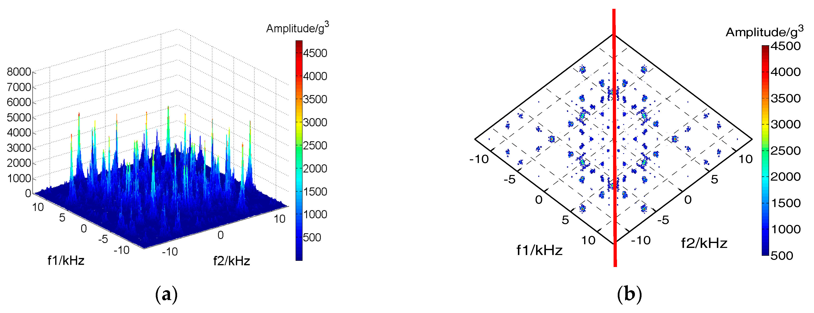
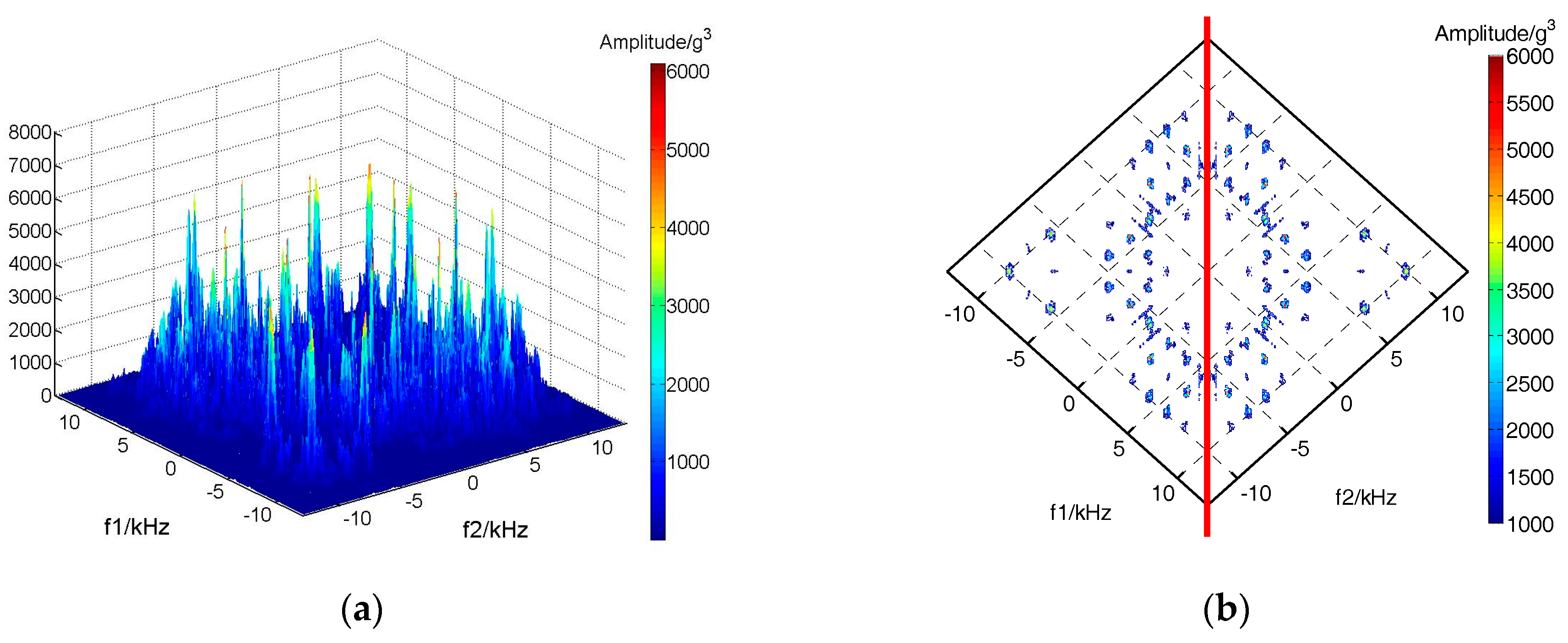
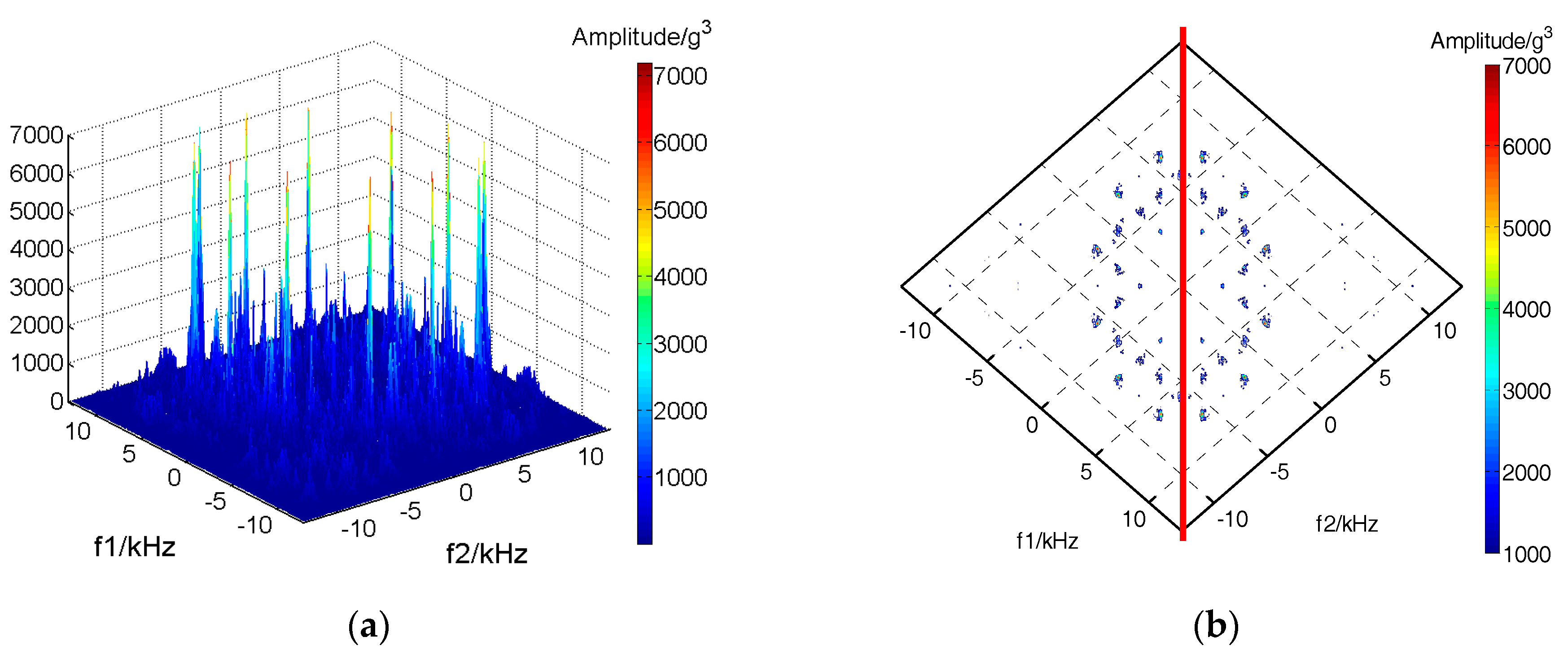
In order to further analyze the characteristics of valve clearance in different states, the bispectrum analysis of reconstructed signal was carried out. The results are shown in Figure 11, Figure 12 and Figure 13. Figure 11a, Figure 12a and Figure 13a are three-dimensional bispectrum diagrams, and Figure 11b, Figure 12b and Figure 13b are bispectrum contour diagrams. From the results, we can find that the bispectrum amplitude is not zero, and the peak value appears at some frequencies, which indicates that the cylinder head vibration signal is non-Gauss signal, and the phenomenon of quadratic phase coupling exists. The second phase coupling phenomenon is the most common nonlinear phenomenon. So, the vibration signal is also a nonlinear signal. From the figures it can be found that the peak value of bispectrum image is gradually increasing from the smaller valve clearance to the bigger valve clearance, which indicates that the nonlinear characteristics of cylinder head vibration signals change with the valve clearance changes. The nonlinearity of cylinder head system increases with the increase of valve clearance (due to wear and deformation of the working parts).
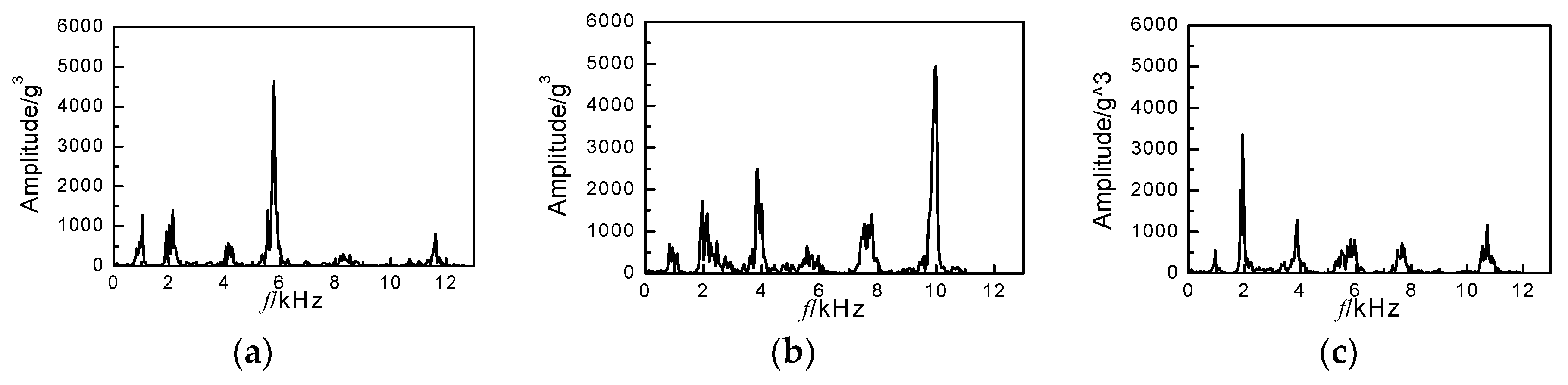
After bispectrum analysis, to further calculate the fault degree by quantization, we need to slice the bispectrum graph diagonally (the angle shown by the red line in the Figure 13b), and analyze it by using the two-dimensional slice data. The two-dimensional slice results are shown in Figure 14.
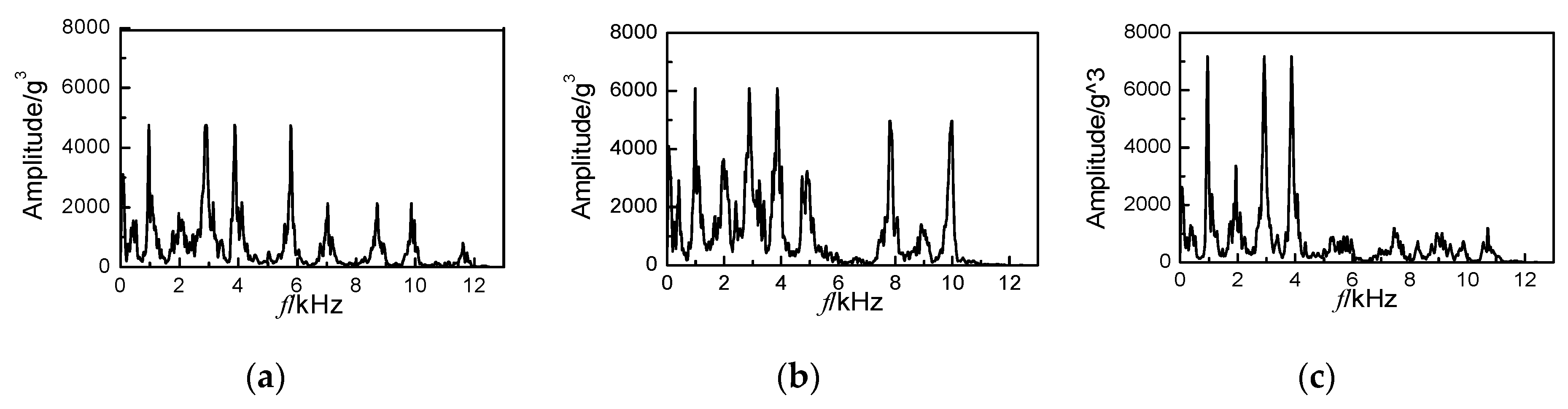
Comparing Figure 14 with Figure 11, Figure 12 and Figure 13, we can find that the diagonal slice method does lead to loss of information. However, the characteristic components should be maintained as far as possible when extracting features from engine vibration signals. So, the diagonal projection method is proposed in this paper, processing the signals with bispectrum to obtain the result as per Figure 11, Figure 12 and Figure 13 preliminarily, then projecting one side of this result on the diagonal line (the red line). All of the subsequent processes will be analyzed based on the diagonal projection. There are two points that should be explained in particular. One is that the result of bispectrum is symmetric and the side selection has no effect on subsequent process. In this paper, the right side was selected. The other one is that the diagonal projection means take the maximum values of every line which is perpendicular to the diagonal projection line instead of taking the sum. The results of diagonal projection are shown as follows:
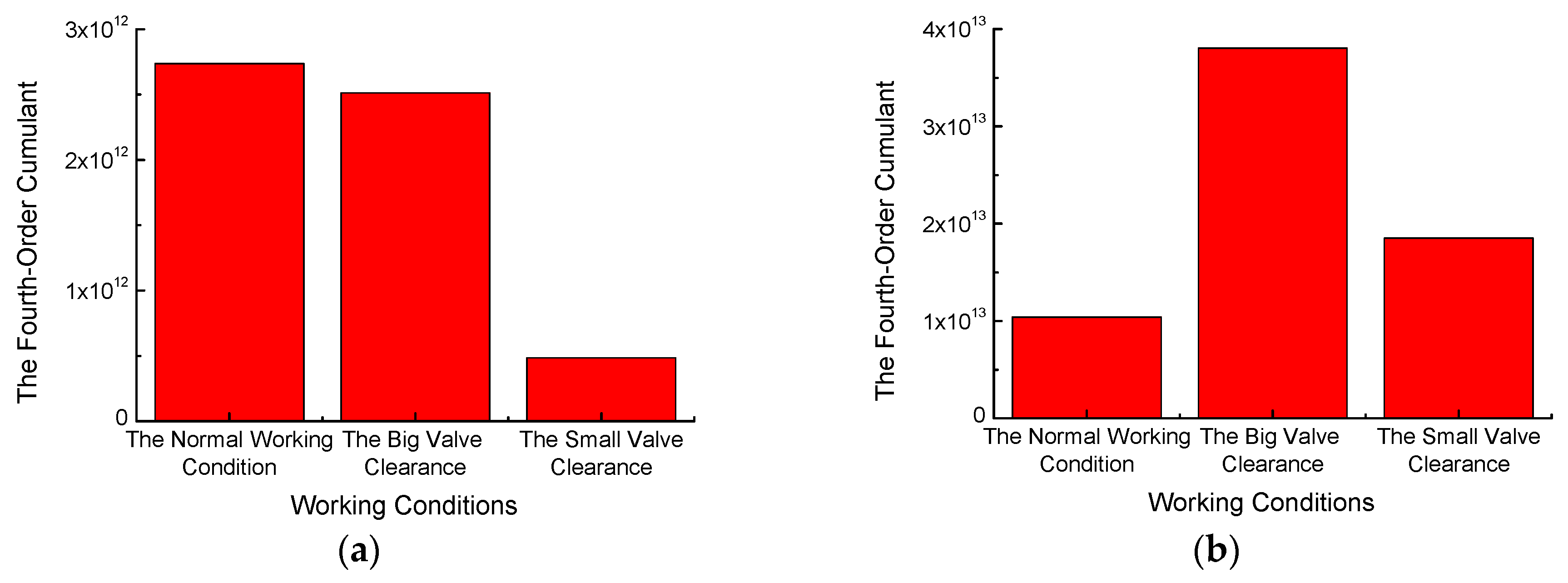
To verify the superiority of this method, 80 segments of cylinder head vibration signals of small valve clearance, normal working conditions, and big valve clearance, respectively, obtained from the test engine as mentioned above were used. Firstly, signals are denoised by VMD. Secondly, the bispectrum is used to analyze those signals preliminarily. Thirdly, the diagonal slice and diagonal projection methods are employed to process bispectrum results, respectively. Finally, the fourth-order cumulants of diagonal slice and diagonal projection are used as an index to detect faults. In order to observe the general recognition performance, all of the 80 sets of signals are processed by mean. The results are shown in Figure 16.
For further comparison, the data normalization is shown in Table 4.
As shown above, the diagonal slice method can recognize small valve clearance easily, but can hardly recognize big valve clearance from normal working conditions. For the diagonal projection method, these three working conditions can be clearly recognized. The normalization results also show that the discrimination of the diagonal projection method is better.
5. Summary and Outlook
This paper presented a new fault diagnosis method for diesel engines based on improved VMD, bispectrum and fourth-order cumulant that employs a cylinder head vibration signal. The research results indicate that the valve clearance fault characteristics can be extracted from the vibration signals clearly.
(1) For the decomposition level selection of VMD, a method based on fluctuation degree of every component’s frequency is proposed in this paper. The results show that using this method the denoising effect is very good. The noise component in the improved reconstructed signal is very small, and the main components of the original signal are preserved in the maximum extent.
(2) For information loss of the bispectrum diagonal slice, a diagonal projection method is proposed in this paper. The analysis results of VMD reconstructed signal show that the diagonal projection method can maintain more information of originals.
(3) Finally, the fourth-order cumulants of diagonal projection are used as an index to detect faults. The results show that three valve states working conditions can be recognized clearly.
However, there are some problems to be solved in following work:
(1) In all of the VMD results, the last component frequency of has a great degree of fluctuation, which is caused by complex vibration source at that frequency. However, it is necessary to optimize VMD in order to get low fluctuation degree in every component.
(2) As shown in Figure 16, in the diagonal slice method, the fourth-order cumulant of normal working conditions is maximum and followed by big valve clearance and small valve clearance. However, the maximum fourth-order cumulant in diagonal projection method is the big valve clearance condition and followed by the small valve clearance and normal working conditions. More information in the diagonal projection method is thought to be the main reason, but the exact component is unclear and needs further study.
(3) In this article, the proposed method is used in the valve clearance fault diagnosis of a diesel engine. In the future, we will continue carrying out experiments and calculations on other types of diesel engine faults. After that, we will improve upon the proposed method to extend this approach to fault diagnosis for other machinery.
Author Contributions
Conceptualization, project administration and funding acquisition, S.C.; methodology, experiments and data analysis, X.B.; academic guidance, resources and supervision, S.C. and D.Z.; writing—original draft, X.B.; writing—review and editing, S.C. and D.Z.
Funding
This research was funded by National Science and Technology Support Program of China, grant number 2015BAF07B04.
Acknowledgments
The authors gratefully acknowledge the financial support provided by the National Science and Technology Support Program of China (No. 2015BAF07B04).
Conflicts of Interest
The authors declare no conflict of interest.
References
- Yu, L.; Junhong, Z.; Fengrong, B.; Lin, J.; Ma, W. A fault diagnosis approach for diesel engine valve train based on improved ITD and SDAG-RVM. Meas. Sci. Technol. 2015, 26, 025003. [Google Scholar] [CrossRef]
- Vulli, S.; Dunne, J.F.; Potenza, R.; Richardson, D.; King, P. Time-frequency analysis of single-point engine-block vibration measurements for multiple excitation-event identification. J. Sound Vib. 2009, 321, 1129–1143. [Google Scholar] [CrossRef]
- Wang, X.; Liu, C.; Bi, F.; Bi, X.; Shao, K. Fault diagnosis of diesel engine based on adaptive wavelet packets and EEMD-fractal dimension. Mech. Syst. Signal Process. 2013, 41, 581–597. [Google Scholar] [CrossRef]
- Liu, Y.; Zhang, J.; Ma, L. A fault diagnosis approach for diesel engines based on self-adaptive WVD, improved FCBF and PECOC-RVM. Neurocomputing 2016, 177, 600–611. [Google Scholar] [CrossRef]
- Antoni, J.; Daniere, J.; Guillet, F. Effective vibration analysis of IC engine using cyclostationarity Part I: A methodology for condition monitoring. J. Sound Vib. 2002, 257, 815–837. [Google Scholar] [CrossRef]
- Lin, J.; Qu, L. Feature extraction based on Morlet wavelet and its application for mechanical fault diagnosis. J. Sound Vib. 2000, 234, 135–148. [Google Scholar] [CrossRef]
- Cai, Y.; Li, A.; He, Y.; Wang, T.; Zhao, J. Application of wavelet packets and GA-BP algorithm in fault diagnosis for diesel valve gap abnormal fault. In Proceedings of the 2010 2nd International Conference on Advanced Computer Control, Shenyang, China, 27–29 March 2010. [Google Scholar]
- Deng, W.; Zhang, S.; Zhao, H.; Yang, X. A Novel Fault Diagnosis Method Based on Integrating Empirical Wavelet Transform and Fuzzy Entropy for Motor Bearing. IEEE Access 2018, 6, 35042–35056. [Google Scholar] [CrossRef]
- Zhang, J.; Yu, L. Bearing fault diagnosis based on improved LMD. In Proceedings of the International Conference on Transportation, Mechanical, and Electrical Engineering, Changchun, China, 16–18 December 2012; pp. 2544–2547. [Google Scholar]
- Zhang, S.; Wang, Y.; He, S.; Jiang, Z. Bearing fault diagnosis based on variational mode decomposition and total variation denoising. Meas. Sci. Technol. 2016, 27, 075101. [Google Scholar] [CrossRef]
- Wu, Z.; Huang, N.E. Ensemble empirical mode decomposition: A noise-assisted data analysis method. Adv. Adapt. Data Anal. 2009, 1, 1–41. [Google Scholar] [CrossRef]
- Dragomiretskiy, K.; Zosso, D. Variational Mode Decomposition. IEEE Trans. Signal Process. 2014, 62, 531–544. [Google Scholar] [CrossRef]
- Zhao, X.; Zhang, S.; Zhishen, L.I.; Fucai, L.I.; Yue, H.U. Application of New Denoising Method Based on VMD in Fault Feature Extraction. J. Vib. Meas. Diagn. 2018, 38, 11–19. [Google Scholar]
- Ma, Z.Q.; Liu, X.Y.; Zhang, J.J.; Wang, J. Application of VMD-ICA combined method in fault diagnosis of rolling bearings. J. Vib. Shock 2017, 36, 201–207. [Google Scholar]
- Mohanty, S.; Gupta, K.K.; Raju, K.S. Comparative study between VMD and EMD in bearing fault diagnosis. In Proceedings of the International Conference on Industrial & Information Systems, Gwalior, India, 15–17 December 2015. [Google Scholar]
- Zhang, J.; Liu, C.W.; Bi, F.R.; Bi, X.B.; Yang, X. Fault Feature Extraction of Diesel Engine Based on Bispectrum Image Fractal Dimension. Chin. J. Mech. Eng. 2018, 31, 216–226. [Google Scholar] [CrossRef]
- Gu, F.; Shao, Y.; Hu, N.; Fazenda, B.; Ball, A. Motor current signal analysis using a modified bispectrum for machine fault diagnosis. In Proceedings of the 2009 ICCAS-SICE, Fukuoka, Japan, 18–21 August 2009; pp. 4890–4895. [Google Scholar]
- Gu, F.; Shao, Y.; Hu, N.; Naid, A.; Ball, A.D. Electrical motor current signal analysis using a modified bispectrum for fault diagnosis of downstream mechanical equipment. Mech. Syst. Signal Process. 2011, 25, 360–372. [Google Scholar] [CrossRef]
- Shen, G.; Stephen, M.; Xu, Y.; Paul, W. Theoretical and experimental analysis of bispectrum of vibration signals for fault diagnosis of gears. Mech. Syst. Signal Process. 2014, 43, 76–89. [Google Scholar]
- Feng, F.; Si, A.; Zhang, H. Research on Fault Diagnosis of Diesel Engine Based on Bispectrum Analysis and Genetic Neural Network. Procedia Eng. 2011, 15, 2454–2458. [Google Scholar] [CrossRef] [Green Version]
- Liang, B.; Iwnicki, S.D.; Zhao, Y. Application of power spectrum, cepstrum, higher order spectrum and neural network analyses for induction motor fault diagnosis. Mech. Syst. Signal Process. 2013, 39, 342–360. [Google Scholar] [CrossRef] [Green Version]
Figure 1.
The analog signal.

Figure 2.
Analog signal decomposition results: (a) VMD decomposition result; (b) EMD decomposition result.
Figure 2.
Analog signal decomposition results: (a) VMD decomposition result; (b) EMD decomposition result.

Figure 3.
Experimental setup. (a) Test engine and the location of acceleration sensors; (b) Dynamometer and LMS Scada III test system.
Figure 3.
Experimental setup. (a) Test engine and the location of acceleration sensors; (b) Dynamometer and LMS Scada III test system.

Figure 4.
Valve clearance small condition: (a) Time waveforms of vibration signals; (b) vibration PSD result.
Figure 4.
Valve clearance small condition: (a) Time waveforms of vibration signals; (b) vibration PSD result.

Figure 5.
Valve clearance normal condition: (a) Time waveforms of vibration signals; (b) Vibration PSD result.
Figure 5.
Valve clearance normal condition: (a) Time waveforms of vibration signals; (b) Vibration PSD result.

Figure 6.
Valve clearance big condition: (a) Time waveforms of vibration signals; (b) Vibration PSD result.
Figure 6.
Valve clearance big condition: (a) Time waveforms of vibration signals; (b) Vibration PSD result.

Figure 7.
Fourth-order cumulant of central frequency of each order component: (a) decomposition layer K = 5; (b) decomposition layer K = 6; (c) decomposition layer K = 7; (d) decomposition layer K = 8.
Figure 7.
Fourth-order cumulant of central frequency of each order component: (a) decomposition layer K = 5; (b) decomposition layer K = 6; (c) decomposition layer K = 7; (d) decomposition layer K = 8.

Figure 8.
Signals of valve clearance small condition: (a) Time waveforms of reconstructed signals; (b) Frequency waveforms of reconstructed signals; (c) Frequency waveforms of original signals. (d) Frequency waveforms of wavelet-denoising signals.
Figure 8.
Signals of valve clearance small condition: (a) Time waveforms of reconstructed signals; (b) Frequency waveforms of reconstructed signals; (c) Frequency waveforms of original signals. (d) Frequency waveforms of wavelet-denoising signals.

Figure 9.
Signals of valve clearance normal condition: (a) Time waveforms of reconstructed signals; (b) Frequency waveforms of reconstructed signals; (c) Frequency waveforms of original signals. (d) Frequency waveforms of wavelet-denoising signals.
Figure 9.
Signals of valve clearance normal condition: (a) Time waveforms of reconstructed signals; (b) Frequency waveforms of reconstructed signals; (c) Frequency waveforms of original signals. (d) Frequency waveforms of wavelet-denoising signals.

Figure 10.
Signals of valve clearance big condition: (a) Time waveforms of reconstructed signals; (b) Frequency waveforms of reconstructed signals; (c) Frequency waveforms of original signals. (d) Frequency waveforms of wavelet-denoising signals.
Figure 10.
Signals of valve clearance big condition: (a) Time waveforms of reconstructed signals; (b) Frequency waveforms of reconstructed signals; (c) Frequency waveforms of original signals. (d) Frequency waveforms of wavelet-denoising signals.

Figure 11.
The bispectrum results of small valve clearance working condition: (a) The 3-dimensional graph; (b) The contour map.
Figure 11.
The bispectrum results of small valve clearance working condition: (a) The 3-dimensional graph; (b) The contour map.

Figure 12.
The bispectrum results of normal working condition: (a) The 3-dimensional graph; (b) The contour map.
Figure 12.
The bispectrum results of normal working condition: (a) The 3-dimensional graph; (b) The contour map.

Figure 13.
The bispectrum results of big valve clearance working condition: (a) The 3-dimensional graph; (b) The contour map.
Figure 13.
The bispectrum results of big valve clearance working condition: (a) The 3-dimensional graph; (b) The contour map.

Figure 14.
The results of diagonal slice. (a) The small valve clearance. (b) The normal working condition. (c) The big valve clearance.
Figure 14.
The results of diagonal slice. (a) The small valve clearance. (b) The normal working condition. (c) The big valve clearance.

Figure 15.
The results of diagonal projection. (a) The small valve clearance. (b) The normal working condition. (c) The big valve clearance.
Figure 15.
The results of diagonal projection. (a) The small valve clearance. (b) The normal working condition. (c) The big valve clearance.

Figure 16.
The calculation results of fourth-order cumulants. (a) The diagonal slice method. (b) The diagonal projection method.
Figure 16.
The calculation results of fourth-order cumulants. (a) The diagonal slice method. (b) The diagonal projection method.


Table 1.
Diesel engine valve clearance fault conditions.
| Condition | Intake Valve Clearance (mm) | Exhaust Valve Clearance (mm) |
|---|---|---|
| Clearance small | 0.25 | 0.45 |
| Clearance normal | 0.3 | 0.5 |
| Clearance big | 0.35 | 0.55 |
Table 2.
The fourth-order cumulant result under different decomposition layer K.
| Decomposition Layer K | 5 | 6 | 7 | 8 |
|---|---|---|---|---|
| Fourth-order cumulant | 6.75 × 10⁹ | 5.52 × 10⁹ | 1.36 × 10¹⁰ | −5.9 × 10¹⁰ |
Table 3.
The results of EAverage.
| Working Condition | Original Signal | VMD Reconstructed | Wavelet Denoising |
|---|---|---|---|
| Normal working condition | 109.77 | 69.64 | 43.55 |
| Big valve clearance | 80.73 | 50.93 | 20.33 |
| Small valve clearance | 91.39 | 57.96 | 18.03 |
Table 4.
The results of normalization.
| Working Condition | Diagonal Section | Diagonal Projection |
|---|---|---|
| Normal working condition | 1.00 | 0.00 |
| Big valve clearance | 0.90 | 1.00 |
| Small valve clearance | 0.00 | 0.29 |
© 2019 by the authors. Licensee MDPI, Basel, Switzerland. This article is an open access article distributed under the terms and conditions of the Creative Commons Attribution (CC BY) license (http://creativecommons.org/licenses/by/4.0/).
Share and Cite
MDPI and ACS Style
Bi, X.; Cao, S.; Zhang, D. Diesel Engine Valve Clearance Fault Diagnosis Based on Improved Variational Mode Decomposition and Bispectrum. Energies 2019, 12, 661. https://doi.org/10.3390/en12040661
AMA Style
Bi X, Cao S, Zhang D. Diesel Engine Valve Clearance Fault Diagnosis Based on Improved Variational Mode Decomposition and Bispectrum. Energies. 2019; 12(4):661. https://doi.org/10.3390/en12040661
Chicago/Turabian StyleBi, Xiaoyang, Shuqian Cao, and Daming Zhang. 2019. "Diesel Engine Valve Clearance Fault Diagnosis Based on Improved Variational Mode Decomposition and Bispectrum" Energies 12, no. 4: 661. https://doi.org/10.3390/en12040661
Note that from the first issue of 2016, this journal uses article numbers instead of page numbers. See further details here.