Discrete and Continuous Model of Three-Phase Linear Induction Motors “LIMs” Considering Attraction Force


1
Department of Electrical and Electronics Engineering & Computer Sciences, Universidad Nacional de Colombia—Sede Manizales, Cra 27 No. 64 – 60, Manizales, Colombia
2
Unidad Académica de Formación en Ciencias Naturales y Matemáticas, Universidad Católica de Manizales, Cra 23 No. 60 – 63, Manizales, Colombia
3
Facultad de Ciencias—Escuela de Física, Universidad Nacional de Colombia—Sede Medellín, Carrera 65 No. 59A-110, 050034, Medellín, Colombia
*
Author to whom correspondence should be addressed.
Energies 2019, 12(4), 655; https://doi.org/10.3390/en12040655
Submission received: 18 December 2018
/
Revised: 8 February 2019
/
Accepted: 14 February 2019
/
Published: 18 February 2019
(This article belongs to the Section I: Energy Fundamentals and Conversion)
Abstract
:A fifth-order dynamic continuous model of a linear induction motor (LIM), without considering “end effects” and considering attraction force, was developed. The attraction force is necessary in considering the dynamic analysis of the mechanically loaded linear induction motor. To obtain the circuit parameters of the LIM, a physical system was implemented in the laboratory with a Rapid Prototype System. The model was created by modifying the traditional three-phase model of a Y-connected rotary induction motor in a d–q stationary reference frame. The discrete-time LIM model was obtained through the continuous time model solution for its application in simulations or computational solutions in order to analyze nonlinear behaviors and for use in discrete time control systems. To obtain the solution, the continuous time model was divided into a current-fed linear induction motor third-order model, where the current inputs were considered as pseudo-inputs, and a second-order subsystem that only models the currents of the primary with voltages as inputs. For the discrete time model, the current-fed model is discretized by solving a set of differential equations, and the subsystem is discretized by a first-order Taylor series. Finally, a comparison of the continuous and discrete time model behaviors was shown graphically in order to validate the discrete time model.
1. Introduction
Although the linear motor was invented and patented more than a century ago, in the beginning it was impractical due to the difficulty of having a small air gap without roughness and with low power factor efficiency. However, technological advances have given the linear induction motor (LIM) greater importance at the academic and industrial levels, and its use has been extended in many applications [1,2,3,4,5].
When the topological characteristics of an electric machine are modified, such as the development of the LIM from a rotating electric machine, the operating conditions and design criteria differ. The magnetic circuit of the machine introduces new phenomena that cannot be fully explained with conventional theory. Consequently, old methods of analysis have been modified and, sometimes, new theories developed [1,3].
Before the advent of linear motors, rotary motors with rotational-to-linear motion converters and with full mechanical transmissions were used to produce straight line movement. Using linear motors for applications that require linear motion eliminates gears and other mechanisms. The advantages of LIMs applied to linear movement are, among others, high capacity to perform acceleration and deceleration, ability to work in hostile environments, gears and mechanical transmissions are avoided, great ease of control of thrust and speed, existence of normal forces that can be used in levitation, low maintenance cost, low noise, great versatility in negotiating sharp curves and steep slopes, ability to exert force on the secondary without mechanical contact, movement and braking independent of the terrain, and low pollution [6,7,8,9,10]. The regulation problem for rotary induction motors (RIMs) began with the pioneering work of Blaschke [11] in the field-oriented control (FOC), which has become a classical technique for induction motor control. More recently, however, various nonlinear control design approaches have been applied to induction motors in order to improve their performance, including adaptive input/output linearization [12], adaptive backstepping [13], and sliding modes [14,15,16]. With respect to the regulation theory, there are few works related to the regulation or sliding-mode regulation of linear induction motors. All these approaches require full state measurement. Because secondary (linoric) flux is not usually measurable, some researchers have bypassed the problem using flux observers [17,18,19].
With respect to the sampling of rotary induction motor (RIM) dynamics, Ortega and Taoutaou [20], in an effort to implement an FOC with digital devices and to provide stability analysis, derived an exact discrete-time representation of a current-fed rotary induction motor model, which is a third-order model, using state diffeomorphism. Based on the results presented in [20], Loukianov and Rivera [21] derived an approximated voltage-fed sampled-data model (fifth-order) that included a sliding-mode block control. There are few works on sampling LIM dynamics; therefore, it is of great significance to investigate an exact sampled-data representation of full linear induction motor dynamics (fifth-order model), and to design exact discrete-time sliding-mode controllers.
Rong-Jong Wai and Wei-Kuo Liu in [18] describe a nonlinear control strategy to control an LIM servo drive for periodic motion, based on the concept of the nonlinear state feedback theory and optimal technique, which comprises an adaptive optimal control system and a sliding-mode flux observation system. The control and estimation methodologies are derived in the sense of the Lyapunov theorem so that the stability of the control system can be guaranteed. The sliding-mode flux observation system is implemented using a digital signal processor with a high sampling rate to make it possible to achieve good dynamics.
Ezio F. Da Silva et al. [22,23] present a mathematical model that describes the dynamic behavior of an LIM, divided into two portions. The first part represents the model dynamic of conventional induction without the end effects, while the second portion describes the attenuation caused by the end effects on LIM.
In [24], V. H. Benítez et al. present a method to control an LIM using dynamic neural networks. They propose a neural identifier of triangle form and design a reduced-order observer in order to estimate the secondary fluxes. A sliding-mode control is developed to track velocity and flux magnitude.
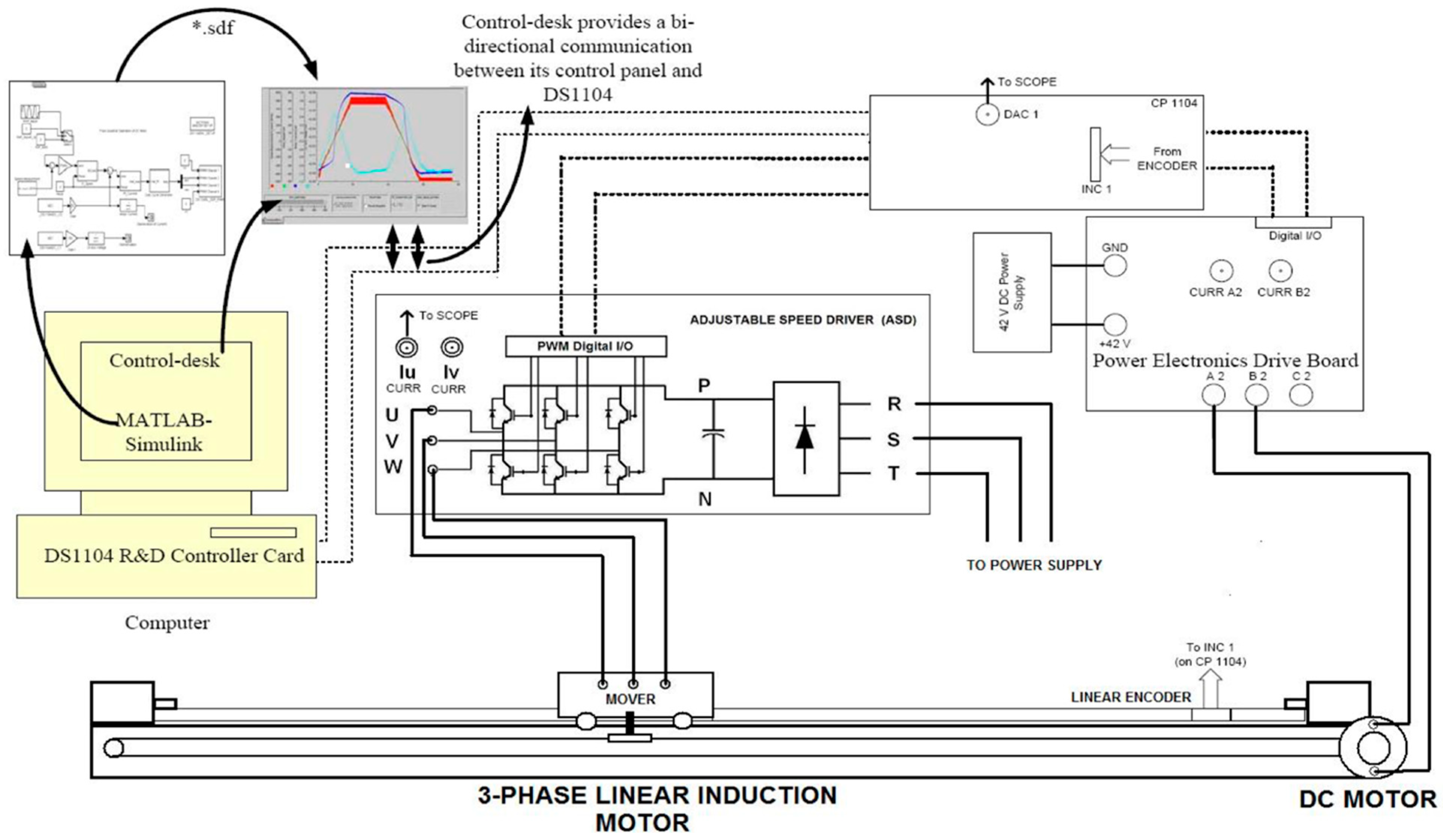
For the development of the model, the physical system was implemented to obtain the parameters of the LIM. The system is illustrated in Figure 1, where there are four important blocks: a controller card, and ASD (adjustable speed driver) that acts a power source of the LIM, a power electronics drive board to feed the DC motor that moves the LIM without load, and the linear induction motor with the measure system.
In Figure 1, the Control-desk with the DS1104 R&D Controller Card serves to generate the PWM to control the ASD to feed the mover of the LIM, as well as capture and store the signals of the different sensors in the motor. All the control system components of the ASD and Power Electronic Drive Board are implemented in Matlab-Simulink® (Versión R2008, The MathWorks, Inc, Natick, MA, USA) [26]. The DC motor, controlled by a Power Electronics Drive Board [27,28] mechanically connected to the LIM, serves to generate movement in the mover without load. That is, the LIM has its power supply but does not spend energy to move itself. In this way, the energy spent by the mover is only the power dissipated by the circuit parameters as losses, allowing the determination of these parameters [25].
This document is organized as follows. The second section presents the principal aspects in the construction of LIMs and their principles of functioning. In the third section the LIM model is developed without considering the effects of the boundaries and considering the forces of attraction. This model was discretized in order to validate the continuous model. In the fourth section we compare the continuous and the discrete models. In the final section we present the conclusions of the work.
2. Construction Aspects of Linear Induction Motors (LIMs)
Linear induction machines are being actively investigated for use in high-speed ground transportation. Other applications, including liquid metal pumps, magnetohydrodynamic power generation, conveyors, cranes, baggage handling systems, as well as a variety of consumer applications, have contributed to an upsurge in interest in LIMs. Unfortunately, the analysis of LIMs is complicated by the so-called “end effect.” In a conventional round-rotor induction motor, the behavior of the machine needs to be calculated only over one pole pitch. The solution for the remaining pole pitches can then be simply obtained by symmetry. However, the symmetry argument cannot be used for a linear machine because the electrical conditions change at the entrance and exit. A more detailed analysis is required to adequately describe its behavior [29].
In principle, for each rotary induction motor (RIM) there is a linear motion counterpart. The imaginary process of cutting and unrolling the rotary machine to obtain the linear induction motor (LIM) is the classic approach (Figure 2). The primary component may now be shorter or larger than the secondary. The shorter component will be the mover. In Figure 2 the secondary component is the mover. The primary component may be double-sided or single-sided.
The secondary material is copper or aluminum for a double-sided LIM, and it may be aluminum (copper) on solid iron for a single-sided LIM. Alternatively, a ladder conductor secondary component placed in the slots of a laminated core may be used for cage rotor RIMs (Figure 1). This latter case is typical for short travel (up to a few meters) and low speed (below 3 m/s) applications. The primary winding produces an airgap field with a strong travelling component at the linear speed v. Linear speed v is defined as:
The number of pole pairs does not influence the ideal no-load linear speed. Incidentally, the peripheral ideal no-load speed in RIMs has the same Formula (1) where is the pole pitch (the spatial semi-period of the travelling field) [30].
3. LIM Model Without End Effects and Considering Attraction Force
The dynamic model of the LIM was modified from the traditional three-phase, Y-connected rotary induction motor in a stationary reference frame [29] and can be described, without end effects and considering attraction force, by the following differential equations [17,30,31]:
where is the mover linear velocity; and are the d-axis and q-axis secondary flux; and are the d-axis and q-axis primary current; and are the d-axis and q-axis primary voltage; is the secondary time constant and it is equal to ; is the leakage coefficient; is the force constant; is the winding resistance per phase; is the secondary resistance per phase referred primary; is the magnetizing inductance per phase; is the secondary inductance per phase referred; is the primary inductance per phase; is the external force disturbance; is the total mass of the mover; is the viscous friction; and is the pole pitch.
To distinguish a stationary reference frame model, we changed the notation to obtain an “ model”. We changed the and indexes to and , respectively, and we omitted the primary and secondary components because the voltages and currents are represented by the primary component, and the fluxes are represented by the secondary component.
The discrete time model of the LIM was obtained through the continuous time model solution. To overcome this problem, the continuous time model was divided into a current-fed linear induction motor third-order model, where the current inputs were considered as pseudo-inputs, and a second-order subsystem that only models the currents of the primary, with voltages as inputs. The current-fed model was exactly discretized by solving a set of differential equations, and the other subsystem was discretized by a first-order Taylor series. The currents subsystem with voltages as inputs is given by Equation (4):
The current-fed induction motor third-order model is given by Equation (5):
The following matrices are defined in order to simplify notation:
Then, the simplified third-order model is Equation (6):
The following variables were changed:
where is the mover linear displacement.
The exponential factor in the transformation is:
Applying this transformation to system (6), we obtained the bilinear model Equation (7):
The first equation in Equation (7) is in the form of Equation (8) with :
Multiplying the differential Equation (8) by the integral factor yields:
Integrating Equation (9), and considering that input is always constant during the integration interval time yields:
With , the first equation solution in Equation (7) is:
Electromechanical equations are then used as follows:
Multiplying the differential Equation (12) by the integral factor yields:
Integrating Equation (13), and considering that input is always constant during the integration interval time yields:
To solve the integral in Equation (14), where is a dummy integration variable, Equation (10) is used with and (skew-symmetry of ):
The velocity mechanical Equation (12) solution is:
Solutions to the bilinear model system Equation (7) were found from an initial time to an arbitrary time :
Equation (15) was integrated in order to obtain the mover position:
In a general form, the initial time is and states are found in a time. In discrete time systems, is the sample time. Common notations are defined as:
Using the above notation in Equations (16) and (17), we have:
System (18) is a transformed discrete-time version of Equation (5) (with the position mover added). To return back to original states, we made a backward transformation using the following change of coordinates:
to obtain
where:
To discretize the differential equations of the current, we used the backward difference method. Finally, the discrete time version of the linear induction motor model is featured:
4. Results and Analysis
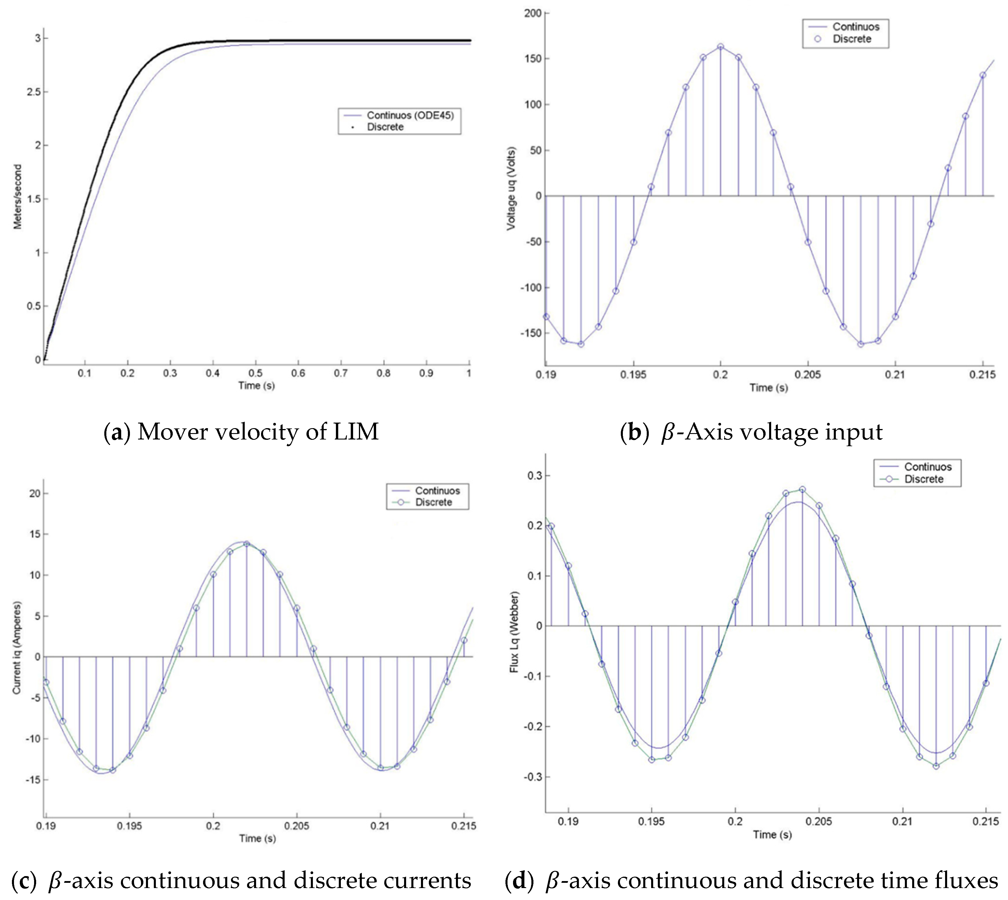
Discrete vs. continuous time model simulation results are shown in Figure 3, which refers to the transformation axis. Figure 3a illustrates the mover velocity of the LIM, or the secondary in the transient and steady states showing lower velocity in the continuous model. Figure 3b shows the β-Axis voltage input. There was no error in the signals that were taken in the same point of the simulation.
Figure 3c illustrates the β-axis continuous and discrete time currents. The discrete current signal presented a phase delay of approximately 1.25 ms, with respect to the signal of the continuous model, because of the processing time and a drop in a few milliamps.
5. Conclusions
A fifth-order dynamic continuous model of an LIM, without considering end effects and considering attraction force, was obtained by modifying a traditional three-phase model, Y-connected rotary induction motor in a d–q stationary reference frame. The discrete time model of the LIM was obtained by the continuous time model solution. To obtain the solution, the continuous time model was divided into a current-fed linear induction motor third-order model, where the current inputs were considered as pseudo-inputs, and a second-order subsystem that only models the currents of the primary with voltages as inputs. For the discrete time model, the current-fed model was exactly discretized by solving a set of differential equations, and the subsystem was discretized by a first-order Taylor series. Finally, a comparison of continuous and discrete time model behaviors was shown graphically in order to validate the discrete time model. The differences found in the responses of the continuous and the discrete time models were due to approximation of the current in constant form between periods.
Author Contributions
Conceptualization, N.T.-G.; methodology, N.T.-G. and Y.A.G.-G.; software, N.T.-G. and F.E.H.; validation, N.T.-G., Y.A.G.-G. and F.E.H.; formal analysis, N.T.-G.; investigation, Y.A.G.-G. and F.E.H.; writing—original draft preparation, F.E.H.; writing—review and editing, N.T.-G., Y.A.G.-G. and F.E.H.; visualization, Y.A.G.-G.; project administration, N.T.-G.; funding acquisition, N.T.-G.
Funding
This research received no external funding.
Acknowledgments
This work was supported by the Universidad Nacional de Colombia, Sede Medellín, grupo de investigación en Procesamiento Digital de Señales para Sistemas en Tiempo Real under the projects HERMES-34671 and HERMES-36911, and the Universidad Católica de Manizales with the Grupo de Investigación en Desarrollos Tecnológicos y Ambientales GIDTA. The authors thank the School of Physics for their valuable support given to the conduction of this research. This research paper corresponds to “programa reconstrucción del tejido social en zonas de pos-conflicto en Colombia del proyecto Modelo ecosistémico de mejoramiento rural y construcción de paz: instalación de capacidades locales,” and is financed by the “Fondo Nacional de Financiamiento para la Ciencia, la Tecnología, y la Innovación, Fondo Francisco José de Caldas con contrato No 213-2018 con Código 58960.” Programa “Colombia Científica”.
Conflicts of Interest
The authors declare no conflict of interest.
References
- Boldea, I.; Nasar, S.A. Linear Motion Electromagnetic Devices; Taylor & Francis: New York, NY, USA, 5 November 2001. [Google Scholar]
- Boldea, I.; Nasar, S.A. Linear electric actuators and generators. IEEE Trans. Energy Convers. 1999, 14, 712–717. [Google Scholar] [CrossRef]
- Nasar, S.A.; Boldea, I. Linear Electric Motors: Theory, Design and Practical Applications; Prentice Hall Trade: Englewood Cliffs, NJ, USA, February 1987. [Google Scholar]
- Nasar, S.A.; Boldea, I. Linear Motion Electric Machines; John Wiley & Sons Inc.: New York, NY, USA, August 1976. [Google Scholar]
- Boldea, I.; Nasar, S.A. Linear Electric Actuators and Generators; Cambridge University Press: New York, NY, USA, 26 September 2005. [Google Scholar]
- Kang, G.; Nam, K. Field-oriented control scheme for linear induction motor with the end effect. IEE Proc. Electr. Power Appl. 2005, 152, 1565–1572. [Google Scholar] [CrossRef]
- Li, Y.; Wang, K.; Shi, L. On-line parameter identification of linear induction motor based on adaptive observer. In Proceedings of the 2007 International Conference on Electrical Machines and Systems (ICEMS), Seoul, Korea, 8–11 October 2007; pp. 1606–1609. [Google Scholar]
- Xu, W.; Zhu, J.; Guo, Y.; Wang, Y. Equivalent circuits for single-sided linear induction motors. In Proceedings of the 2009 IEEE Energy Conversion Congress and Exposition, San Jose, CA, USA, 20–24 September 2009; pp. 1288–1295. [Google Scholar]
- Du, Y.; Jin, N. Research on characteristics of single-sided linear induction motors for urban transit. In Proceedings of the 2009 International Conference on Electrical Machines and Systems, Tokyo, Japan, 15–18 November 2009; pp. 1–4. [Google Scholar]
- Faiz, J.; Jagari, H. Accurate modeling of single-sided linear induction motor considers end effect and equivalent thickness. IEEE Trans. Magn. 2000, 36, 3785–3790. [Google Scholar] [CrossRef]
- Blaschke, F. The principle of field orientation applied to the new transvector closed-loop control system for rotating field machines. Siemens Rev. 1971, 39, 217–220. [Google Scholar]
- Marino, R.; Tomei, P. Nonlinear Control Design; Prentice Hall: New York, NY, USA, 1995. [Google Scholar]
- Tan, H.; Chang, J. Adaptive backstepping control of induction motor with uncertainties. In Proceedings of the American Control Conference, San Diego, CA, USA, 2–4 June 1999. [Google Scholar]
- Loukianov, G.A.; Cañedo, J.M.; Serrano, O.; Utkin, I.V.; Celikovsky, S. Adaptive Sliding Mode Block Control of Induction Motors; Mc Graw Hill: New York, NY, USA, 1999. [Google Scholar]
- Utkin, V.I.; Guldner, J.; Shi, J. Sliding Mode Control in Electromechanical Systems; Taylor and Francis: London, UK; Philadelphia, PA, USA, 1999. [Google Scholar]
- Dodds, S.J.; Utkin, V.A.; Vittek, J. Self Oscillating, Synchronous Motor Drive Control System with Prescribed Closed-Loop Speed Dynamics. In Proceedings of the 2nd EPE Chapter Symposium on ‘Electric Drive Design and Applications’, Nancy, France, 4–6 June 1996; pp. 23–28. [Google Scholar]
- Wai, R.J.; Liu, W.K. Nonlinear decoupled control for linear induction motor servo-drive using the sliding-mode technique. IEEE Proc. Control Theory Appl. 2001, 148, 217–231. [Google Scholar] [CrossRef]
- Wai, R.J.; Liu, W.K. Non linear control for linear induction motor servo drive. IEEE Trans. Ind. Electron. 2013, 50, 920–935. [Google Scholar]
- Liu, J.; Lin, F.; Yang, Z.; Zheng, T.Q. Field oriented control of linear induction motor considering attraction force and end-effects. In Proceedings of the International Power Electronics and Motion Control Conference IPEMC 2006, Shanghai, China, 14–16 August 2006. [Google Scholar]
- Ortega, R.; Taoutaou, D. A globally stable discrete-time controller for current-fed induction motors. Syst. Control Lett. 1996, 28, 123–128. [Google Scholar] [CrossRef]
- Loukianov, A.G.; Rivera, J.; Cañedo, J.M. Discrete-time sliding mode control of an induction motor. In Proceedings of the 15th World Congress of IFAC, Barcelona, Spain, 21–26 July 2002; Volume 1, pp. 106–111. [Google Scholar]
- Fernandes, E.; dos Santos, C.C.; Lima, J.W. Field oriented control of linear induction motor taking into account end-effects. In Proceedings of the AMC 2004, Kawasaki, Japan, 25 March 2004; pp. 689–694. [Google Scholar]
- Fernandes, E.; dos Santos, E.B.; Machado, P.C.M.; de Oliveira, M.A.A. Dynamic model for linear induction motors. In Proceedings of the ICIT 2003, Maribor, Slovenia, 10–12 December 2003; pp. 478–482. [Google Scholar]
- Benitez, V.H.; Loukianov, A.G.; Sanchez, E.N. Identification and control of a linear induction motor using an α − β model. In Proceedings of the American Control Conference, Denver, CO, USA, 4–6 June 2003. [Google Scholar]
- Toro, N.; Garcés, Y.A.; Hoyos, F.E.; Sanchez, E.N. Parameter Estimation of Linear Induction Motor LabVolt 8228-02. In Proceedings of the Congreso Anual Asociación de Mexico de Control Automático, Saltillo, Mexican, 5–7 December 2011. [Google Scholar]
- Morfin, O.A.; Castañeda, C.E.; Valderrabano-Gonzalez, A.; Hernandez-Gonzalez, M.; Valenzuela, F.A. A Real-Time SOSM Super-Twisting Technique for a Compound DC Motor Velocity Controller. Energies 2017, 10, 1286. [Google Scholar] [CrossRef]
- Hoyos Velasco, F.E.; Candelo-Becerra, J.E.; Rincón Santamaría, A. Dynamic Analysis of a Permanent Magnet DC Motor Using a Buck Converter Controlled by ZAD-FPIC. Energies 2018, 11, 3388. [Google Scholar] [CrossRef]
- Hernández-Márquez, E.; Avila-Rea, C.A.; García-Sánchez, J.R.; Silva-Ortigoza, R.; Silva-Ortigoza, G.; Taud, H.; Marcelino-Aranda, M. Robust Tracking Controller for a DC/DC Buck-Boost Converter–Inverter–DC Motor System. Energies 2018, 11, 2500. [Google Scholar] [CrossRef]
- Lipo, T.A.; Nondahl, T.A. Pole-by-pole d-q model of a linear induction machine. IEEE Trans. Power Appar. Syst. 1979, PAS-98, 629–642. [Google Scholar] [CrossRef]
- Boldea, I.; Nasar, S.A. The Induction Machine Handbook; Electric Power Engineering; CRC Press: Boca Raton, FL, USA, 2002. [Google Scholar]
- Benitez, V.H.; Sanchez, E.N.; Loukianov, A.G. Neural identification and control for linear induction motors. J. Intell. Fuzzy Syst. 2005, 16, 33–55. [Google Scholar]
Figure 1.
Physical system implemented to obtain the linear induction motor (LIM) model parameters [25].
Figure 1.
Physical system implemented to obtain the linear induction motor (LIM) model parameters [25].

Figure 2.
Cutting and unrolling process to obtain an LIM and its various parts.
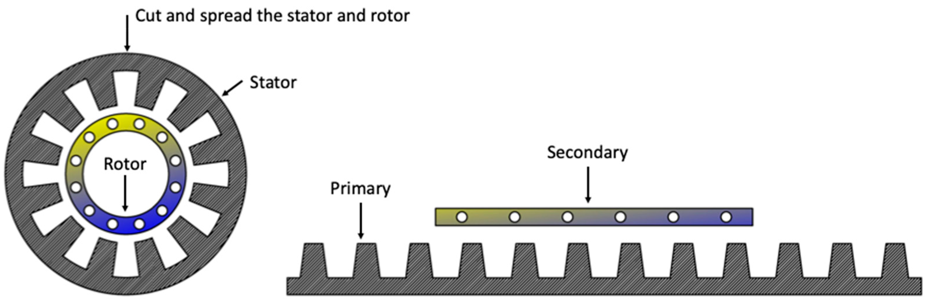
Figure 3.
Mover velocity, voltage, currents, and fluxes resulting from the model simulation using the ODE45 function of Matlab in the continuous and discrete time models of LIM.
Figure 3.
Mover velocity, voltage, currents, and fluxes resulting from the model simulation using the ODE45 function of Matlab in the continuous and discrete time models of LIM.
© 2019 by the authors. Licensee MDPI, Basel, Switzerland. This article is an open access article distributed under the terms and conditions of the Creative Commons Attribution (CC BY) license (http://creativecommons.org/licenses/by/4.0/).
Share and Cite
MDPI and ACS Style
Toro-García, N.; Garcés-Gómez, Y.A.; Hoyos, F.E. Discrete and Continuous Model of Three-Phase Linear Induction Motors “LIMs” Considering Attraction Force. Energies 2019, 12, 655. https://doi.org/10.3390/en12040655
AMA Style
Toro-García N, Garcés-Gómez YA, Hoyos FE. Discrete and Continuous Model of Three-Phase Linear Induction Motors “LIMs” Considering Attraction Force. Energies. 2019; 12(4):655. https://doi.org/10.3390/en12040655
Chicago/Turabian StyleToro-García, Nicolás, Yeison A. Garcés-Gómez, and Fredy E. Hoyos. 2019. "Discrete and Continuous Model of Three-Phase Linear Induction Motors “LIMs” Considering Attraction Force" Energies 12, no. 4: 655. https://doi.org/10.3390/en12040655
Note that from the first issue of 2016, this journal uses article numbers instead of page numbers. See further details here.