Wind Power Integration: An Experimental Investigation for Powering Local Communities
by
 ,
,
Mazhar Hussain Baloch
1,2, 
Dahaman Ishak
1,*,
Sohaib Tahir Chaudary
3,4,
Baqir Ali
2,
Ali Asghar Memon
2 and
Touqeer Ahmed Jumani
2 1
School of Electrical & Electronic Engineering, Universiti Sains Malaysia, 14300 Nibong Tebal, Malaysia
2
Department of Electrical Engineering, Mehran University of Engg & Technology, 76062 Sindh, Pakistan
3
School of Electronic Information & Electrical Engg, Shanghai Jiao Tong University, 200240 Shanghai, China
4
Department of Electrical Engineering, COMSATS University, Islamabad, Sahiwal Campus, 57000 Sahiwal, Pakistan
*
Author to whom correspondence should be addressed.
Energies 2019, 12(4), 621; https://doi.org/10.3390/en12040621
Submission received: 15 January 2019
/
Revised: 8 February 2019
/
Accepted: 12 February 2019
/
Published: 15 February 2019
(This article belongs to the Section C: Energy Economics and Policy)
Abstract
:The incorporation of wind energy as a non-conventional energy source has received a lot of attention. The selection of wind turbine (WT) prototypes and their installation based on assessment and analysis is considered as a major problem. This paper focuses on addressing the aforementioned issues through a Weibull distribution technique based on five different methods. The accurate results are obtained by considering the real-time data of a particular site located in the coastal zone of Pakistan. Based on the computations, it is observed that the proposed site has most suitable wind characteristics, low turbulence intensity, wind shear exponent located in a safe region, adequate generation with the most adequate capacity factor and wind potential. The wind potential of the proposed site is explicitly evaluated with the support of wind rose diagrams at different heights. The energy generated by ten different prototypes will suggest the most optimum and implausible WT models. Correspondingly, the most capricious as well as optimal methods are also classified among the five Weibull parameters. Moreover, this study provides a meaningful course of action for the selection of a suitable site, WT prototype and parameters evaluation based on the real-time data for powering local communities.
1. Introduction
Owing to the escalation in energy demand to meet fundamental life necessities, researchers around the world are trying to find the best ways to employ renewable energy resources. Several techniques are proposed in the literature, different methods are introduced and numerous policies are presented to get an optimum solution. The installation of wind energy resources along the coastline is getting much attention due to the opportunity of integration of both on-shore and off-shore wind farms. In this work Pakistan is considered as an example, due to its 1600 km long coastline and the energy crisis Pakistan is facing, which has badly affected the economy and daily life of its 220 million citizens. The Government of Pakistan has tried many initiatives to reduce load shedding and provide clean, affordable and continuous electric supply. As a result there is a need to explore more available options instead of relying only on traditional fossil fuels. The Alternative Energy Distribution Board (AEDB) has taken serious steps to promote renewable energy by exploring the available wind, solar and hydro energy resource potential. The National Electric Power Regulation Authority (NEPRA) has encouraged the generation of renewable energy by giving letters of intent (LOIs) to many contractors. Figure 1 shows the share of power generation as a percentage of different resources [1]. The country is moving towards sustainable renewable energy resources as compared to past five years, but currently, a significant percentage share in country’s electrical power generation is still based on fossil fuels.
The wind energy potential in Pakistan is the major focus for power generation as renewable energy is a most fundamental necessity to help mankind and meet energy demands, so an analysis of long term pathways for power generation is described in [2]. It is also depicted that compromising on the issues of renewable energy just for the sake of convenience is not a practical approach. Likewise, selection criteria for the most appropriate sites in Pakistan for wind energy generation based on an analytic hierarchal process is described in [3]. An analysis on energy security according to renewable the energy policy of Pakistan is elaborated in [4]. A corresponding research analysis considering the Badin and Pasni territories of Pakistan is presented in [5]. The contemporary development of wind energy, challenges and future recommendations are deliberated in [6]. The wind energy potential and power law assessment in Malaysia, economic value assessment analyzed for an optimal sizing of an energy storage system and integration of digital control techniques based on power electronics converters are described in [7,8,9].
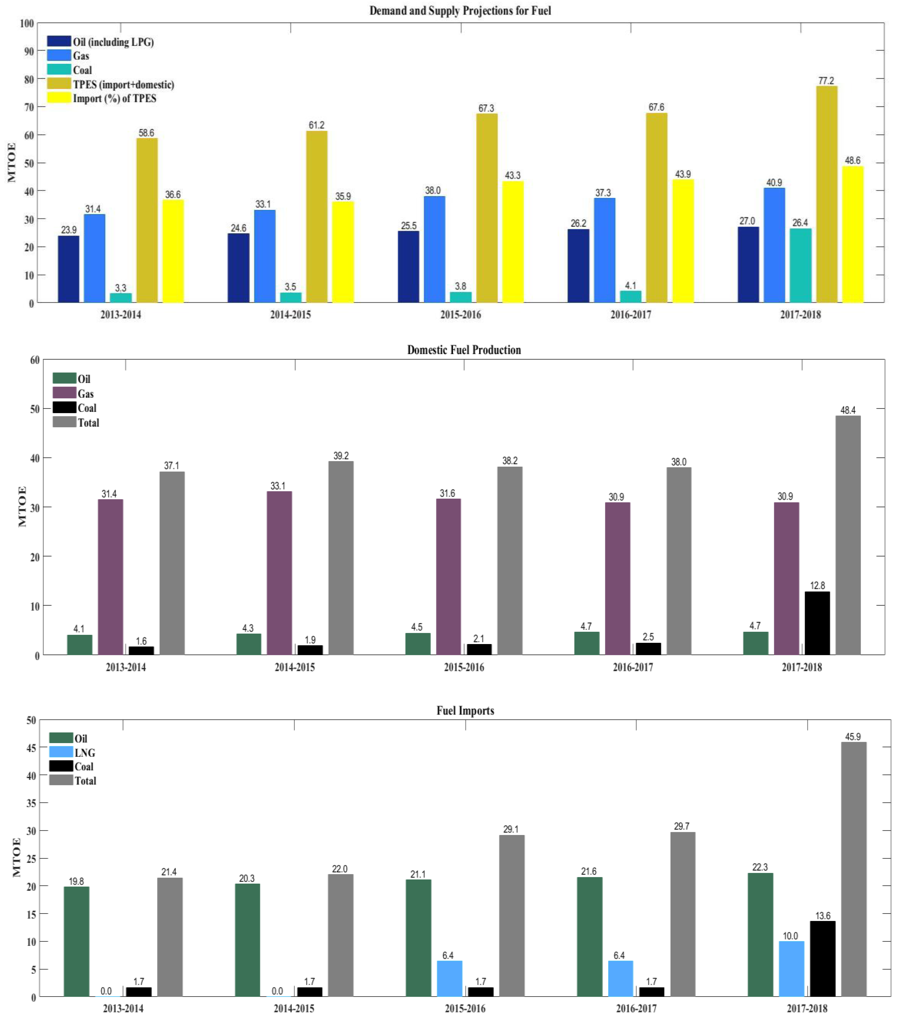
Domestic use, as well as imports of these conventional sources, has put a massive burden on the economy of the country and also caused environmental and health issues. Pakistan has a tremendous wind energy potential available in Sindh and Baluchistan. There is a terrible need for the country to move towards renewable energies like hydro, wind, solar and bioenergy. The Ministry of Planning, Development, and Reforms in Pakistan has taken the initiative under the 11th five-year plan, in which energy crisis is cogitated, and strategies to meet the energy demands of Pakistan have been proposed [1]. Figure 2 shows the demand and supply projections for fuel from 2013 to 2018. Oil (including LPG), gas, coal, total primary energy supply (TPES) and imports as the percentage of TPES resulted in a million tons of oil equivalent (MTOE). In 2017–2018 total domestic fuel produced by Pakistan in MTOE was about 48.43 and fuel imports of 45.87 MTOE. As compared to the previous year 2016–2017, the domestic fuel production increased only 10.45%. Figure 3 shows the per annum demand for power (MW) by NTDC and KESC. During the period of 2017–2018, power demand by National Transmission and Dispatch Company (NTDC) and Karachi Electric Supply Company (KESC) was 26.53 GW and 4.5 GW, respectively.
Total power demand based on the performance of models is tested and evaluated to suggest more accurate Weibull distribution model. One-year data is analyzed for this purpose. Wind characteristics are estimated on the basis of daily as well as monthly average speeds, the WR, air density, WPD, energy in terms of kW/m2, shear exponent coefficient (∝) for boundary layer of the site, and turbulence intensity of the proposed site. Ten different wind turbine models are used to estimate wind power output and energy generated at the proposed site. More capacity factor of each wind turbine is calculated to suggest a more efficient model for this site.
MATLAB is used for the assessment of wind potential at the proposed site. Data is acquired with the support of Pakistan Metrological department (PMD). However, for more accuracy, data quality assurance test is conducted to avoid errors in results, by generating a code which organizes and inspects wind data for errors. The excellent observation data is used to estimate stated parameters. Results suggested that this site has a vast potential for wind energy that can be exploited to meet a moderate portion of energy demand in Pakistan. The proposed site is in premises of 600 kV HVDC line from Matiari to Lahore which is planned up to 2021–2022 under CPEC [10].
In this paper, five different methods based on Weibull distribution techniques have been cogitated. The real time data at various heights from a site located in coastal zone of Pakistan has been employed to acquire different parameters. Based on the calculations and analysis, most optimal wind turbine having ability to be operated on the highest wind potential and most adequate capacity factor is sorted out. The wind potential at the different heights and in proper direction on proposed site is explicitly evaluated through wind rose diagrams. The energy production capacity of ten different prototypes is calculated and the most optimum and implausible WT models are suggested along with their pros. and cons. according to the different wind classes. Congruently, the most improvident as well as finest methods are also rated among five Weibull parameters. Additionally, this paper also provides a significant strategy for the determining an appropriate site, wind turbine prototype and parameters evaluation based on the real-time data with an instance from coastal area of Pakistan for providing electrical energy in the local communities. It is expected that this study will be an imperative contribution in understanding and applying the numerous Weibull distribution techniques and also in selection of wind turbine models by considering various parameters. Therefore, the results will be undoubtedly helpful in making an efficient energy policy in the future.
2. Wind Data Assessment
The characteristics of wind have time a varying nature at each instant. There are various parameters that are key indicators to estimate that whether a particular site is suitable for a utility-scale wind power project [11,12,13].
These parameters are air density, ambient temperature, turbine class and the hub height of turbine at which blades usually capture the wind energy. For accuracy, it is essential to assess wind energy potential of proposed site critically by considering aforementioned wind characteristics. Wind power density is considered as another critical factor in determining how much wind power (W) is available at per unit area (m2) area. This can be achieved by probability distribution function [14]. The wind map of Pakistan is provided in Figure 4, where several wind classes are classified by taking wind power generation into account [13].
2.1. Wind Characteristics
To assess the wind potential of a particular site, it should be considered that wind energy is a time-varying entity which not only changes the magnitude but also the direction [15,16]. Moreover, above characteristics are significant for adequate evaluation of wind potential available in particular site. Wind turbine performance is affected by the wind rose and frequency of wind distribution during the higher occurrence of wind speed [17,18,19,20]. An appropriate method for analyzing the wind characteristics and wind energy potential is referred in [21]. Moreover, if the data for more than two years have been considered, then measure-correlate-predict (MCP) method is clearly described and implemented in [22]. Whereas, the presence of probable errors and accuracy of wind speed data is also discussed in the same article.
2.1.1. Average Wind Speed, Variance and Standard Deviation
The mean or average wind speed ‘’ is obtained from Equation (1). Whereas, the variance ‘’ and standard deviation (SD) ‘’, for wind speed data are calculated from Equations (2) and (3) respectively:
where n is a number of observations, is the i-th wind speed, i is the i-th observation.
2.1.2. Air Density, Wind Power Density and Energy
The air density for the proposed site can be obtained by using Equation (4) [23,24,25], wind power density (WPD) and energy (E) from Equations (5) and (6):
where, is air pressure ( or N/m2), is the specific gas constant (287 J/kg), and is air temperature at the site in Kelvin (C + 273°):
where ρ is the air density, AT is the swept area of turbine blades (m2), Pw is wind power (W), is wind velocity (m/s) and Cp is the Betz limit equal to 0.593 or the maximum value of Cp, the performance for the ideal WT. Furthermore, due to mechanical deficiency of a real turbine, the fraction of the power extracted from the wind will be less than that for an ideal WT. In other words, this limit states how effectively a WT converts the wind energy into electricity [26,27,28]:
where, is energy output in terms of Weibull distribution at the proposed site in (kWh/m2). P(V), T, V, and c are wind turbine’s power curve, time period, wind velocity, shape and scale parameters, respectively [29].
2.1.3. Wind Turbulence Intensity, Shear, and Power Law
Turbulence Intensity (TI) is defined as the ten-minute standard deviation of the velocity divided by the ten-minute mean velocity of the wind as given by Equation (7) [25]:
where is considered a ten-minute (SD) of wind velocity, and is the ten-minute average velocity of the proposed site. The exponent of wind shear and shear of the site is calculated from Equations (8) and (9) respectively [30,31,32]. The term α is essential to estimate wind velocities at higher altitude by processing the wind velocities measured at lower or previous altitudes. The power law is used to calculate wind speed at hub height by using Equation (10) [32]:
where and are heights, and are wind speeds, is the coefficient of wind shear and is the reference height.
2.2. Wind Power Classes
Elliot and Schwartz classified wind power into seven classes, considering the wind speed and power density of a particular site [33,34,35,36,37]. The wind power class 1 and 2 are for rural applications, and class 4 and beyond are for commercial purposes [38,39,40,41]. They defined these classes at heights of 50 m, 30 m, and 10 m [42]. Wind speed above 5.5 m/s yields power generation that is economical and located in class 3. While classes 1 and 2 are for micro-generation purpose [43]. Several parameters regarding wind potential in Pakistan, based on the utility scale of wind class, are articulated in Table 1, which depict that 26,362 km2 of land can be used to produce 131,820 MW of electricity through wind turbines [12]. Whereas, the international standards of wind power generation classification at various heights are categorized in Table 2 [24].
2.3. Weibull Distribution
Weibull distribution of the wind speed data collected from a particular location is a probability density function as well as the cumulative distribution function , it can be calculated from Equations (11) and (12), respectively [44,45,46,47]:
can be calculated as follows:
whereas can be obtained from Equation (14), as given below:
where is a gamma function of , as given by:
2.4. Different Weibull Methods
The shape and scale parameters for Weibull distribution function can be calculated by numerous methods suggested in the literature. In this study five methods namely, GM, MMLM, EPF, EMJ and EML are used in this study to calculate Weibull parameters. In the MMLM method, it is necessary that wind speed data should be in FD format and a number of iterations should be performed to find the shape and scale parameters for Weibull distribution function, which can be obtained from Equations (16) and (17) [48,49]:
In the EML method, Lysen suggested that the shape and scale parameters are obtained from Equations (18) and (19), respectively [50]:
The EMJ, also known as an empirical method of Jestus in which, the shape can be calculated by Equation (18) and scale parameter is calculated by Equation (20) [51,52]:
In the Graphical Method (GM), the cumulative distribution function of Weibull distribution is used, in which wind data is sorted into bins due to the least squares regression. The graphical method’s equation can be obtained by taking double logarithms of Equation (12) [53,54]:
Comparing Equation (20) with , we get:
where, and can be calculated by using measured wind speed data. The standard least regression method is applied to obtain the slope (a) and the intercept , and then the shape and the scale parameters can be determined as:
From EPF, the average wind speed data is considered to calculate shape and scale parameters of the Weibull distribution. First, the parameter for aerodynamic design of the turbine should be defined as [55]:
From Equation (24), the energy pattern factor can be calculated as a ratio of the average of the cubic value of wind speed data over the cubic value of average wind speed data. The shape parameter obtained as [55]:
The scale parameter can be calculated same as Equation (20).
2.5. Goodness of Fit Test
The performance of five Weibull distribution methods is compared by using five statistical analyses, including mean squared error (MSE) given by Equation (26), root mean squared error (RMSE) from Equation (27), mean absolute error (MAE) by using Equation (28), the coefficient of correlation by using Equation (29) and coefficient of determination from Equation (30) as follows:
where represents the i-th actual wind speed, is the i-th predicted wind speed, is mean of the actual wind speed and is the number of observations.
3. Site Characteristics
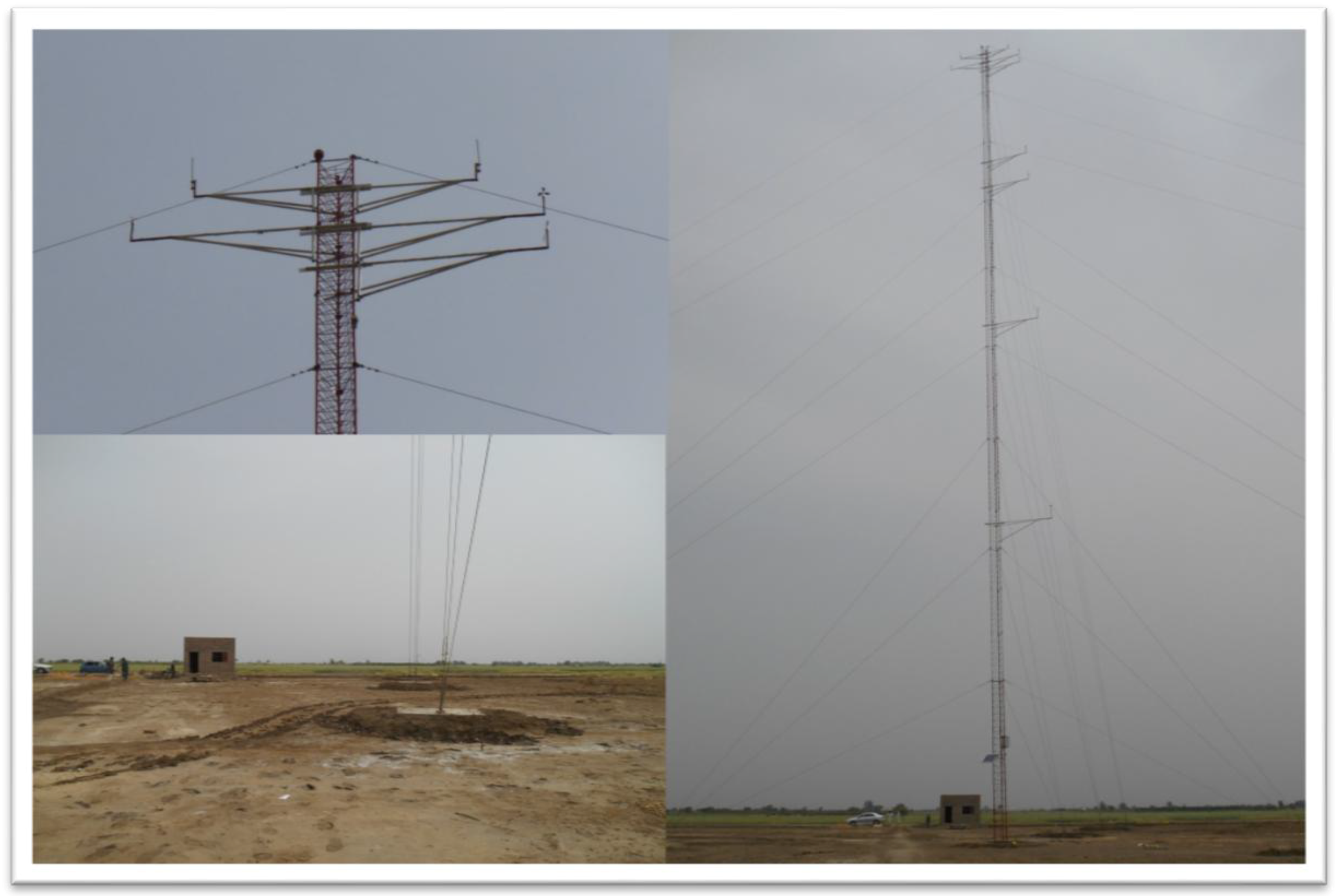
The Sanghar site wind mast funded by the World Bank is located in Sanghar, Sindh, Pakistan. The height of the mast is 80 m, and the geographic location of the site is 25°48′57.26″ N and 69°2′15.12″ E. Figure 5 shows wind mast installed at the Sanghar site with the terrain and surroundings. The proposed site is flat, wide and opens having no obstruction with an elevation higher than 20 m. Figure 6 shows topographic maps for the Sanghar site. The ruggedness index (RIX) at a specific location is the percentage of the ground surface that has a slope above a given threshold (here 30%) within a certain distance (here 3.5 km). The site is located 250 km (4-h drive) away from Jinnah International Airport Karachi, and easily accessible by any type of vehicles. One year 10 min’ average data is analyzed from November 2016 to October 2017.
4. Results and Discussion
4.1. Wind Speed Measurement
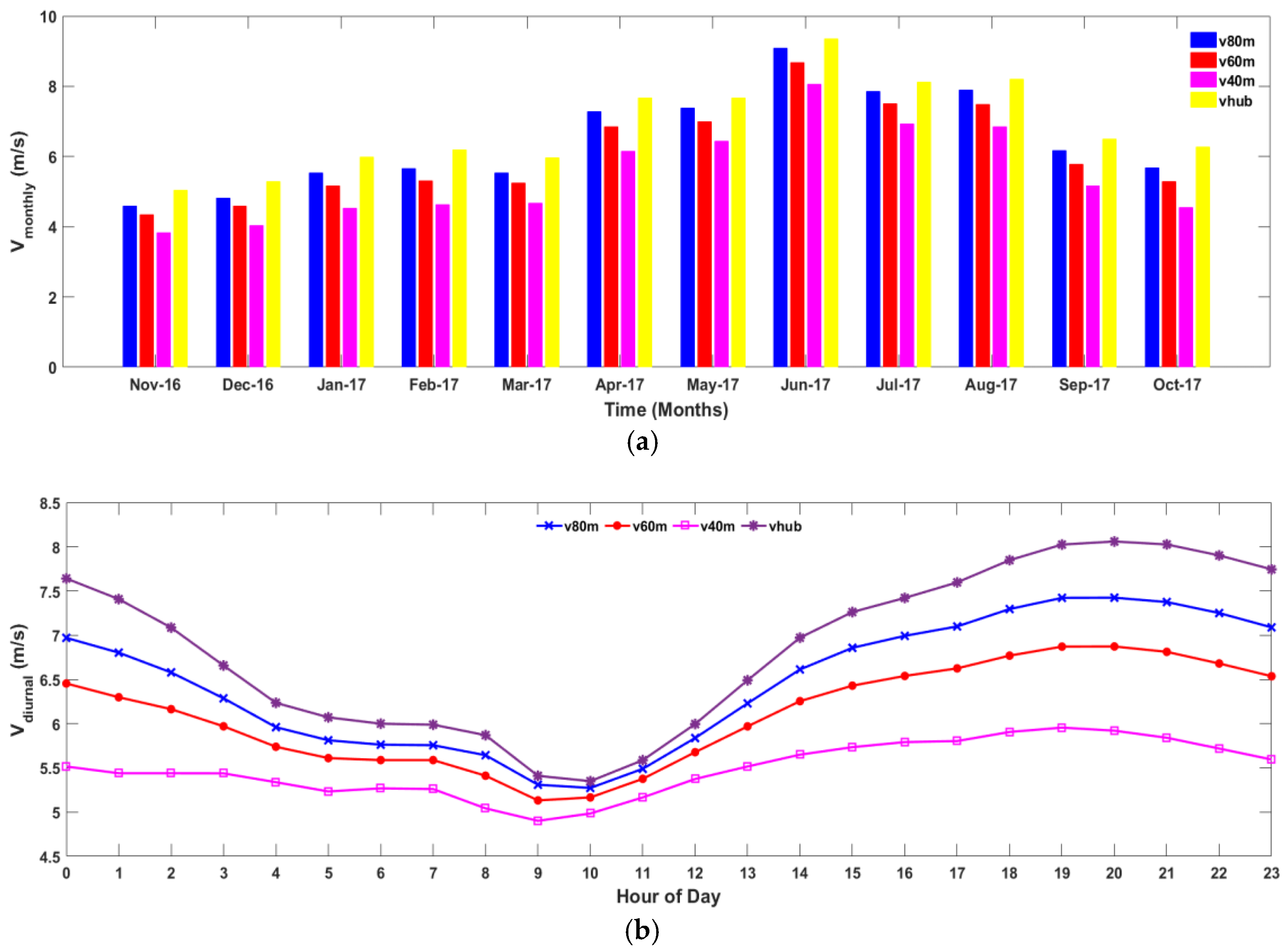
In Figure 7a, monthly average wind speed at different heights, i.e., 100 m, 80 m, 60 m, and 40 m are shown. At a hub height of 100 m, the maximum wind speed is 9.35 m/s in the month of June and minimum 5 m/s in November. Overall wind speed throughout the year is 6.27 m/s, which is suitable for integrating a utility purpose wind plant at the proposed site. Moreover, at the heights of 80 m, 60 m and 40 m the minimum wind speed observed was 4.5 m/s, 4.3 m/s, and 3.8 m/s, respectively, in the month of November, while the maximum wind speed at 80 m, 60 m, and 40 m heights was observed to be 9 m/s, 8.6 m/s, and 8 m/s, respectively, in the month of June. The overall wind speed at these heights observed through the year is 5.6 m/s, 5.2 m/s, and 4.5 m/s, respectively.
Figure 7b shows the diurnal wind speed at this site, with minimum 5.3 m/s at 11 am and maximum 8 m/s from 8 pm to 10 pm at hub height. At heights of 40 m and above, the wind speed lies above 5 m/s throughout the day. For 60 m and above, during the day as well as night time the wind speed lies in wind power class 4 and above.
4.2. Air Density and Turbulence Intensity Measurement
Air density (ρ) is calculated by using temperature, and pressure (Pa) measured at the heights of 76 m and 4 m, respectively. It is a critical factor as it is directly proportional to the wind power density (WPD). 10-min average values for temperature and pressure were used in the estimation of air density to achieve accurate WPD.
In Figure 8, the relation between monthly average of air density and temperature is indicated. The minimum monthly average air density values of about 1.143 kg/m3, 1.14 kg/m3, and 1.147 kg/m3 are observed in the month of May, June, and July respectively. Maximum monthly average air density of about 1.223 kg/m3 is observed in the month of January. Whereas, maximum monthly average temperature of about 30.8 °C, 32.140 °C, and 31.69 °C are observed in the month of April, May, and June, with a minimum of about 16.4 °C in the month of January.
The overall air density (ρ) observed is 1.167 kg/m3, and overall temperature is 27.27 °C. During the summer season, air density is lower than that of the winter season with negligible variation. During the cool-dry winter, hot-dry spring, rainy summer and autumn seasons, the air densities are 1.205 kg/m3, 1.155 kg/m3, 1.148 kg/m3 and 1.1675 kg/m3, respectively.
It can be observed from the topographical map shown in Figure 6 that the roughness length is 0.07 m, corresponding to an open field with distributed rows of trees and low buildings. Roughness length for specific areas is 0.5 m and 0 m for towns and rivers, respectively. Therefore, the site has minimum turbulence and shear. The Turbulence Intensities (TI) at 80 m, 60 m, and 40 m heights are analyzed using 10 min interval yearly data of standard deviation and average wind speed. TI at different heights are shown in Figure 9, which clearly depicts that as altitude rises above ground level from 40 m and above, turbulence intensities are reduced. Therefore, relatively at 80 m or below heights, the wind velocities are more uniform. For the design purpose of a wind turbine, International Electro technical Commission (IEC) has formed standards for TI up to 18%, for a wind speed of 15 m/s, and this site has minimum TI, as perceived in Figure 9.
The use of standard (constant) air density i.e., 1.255 kg/m3 for the analysis can cause the variation of wind power density results [27]. When the wind power density is calculated using the air pressure and temperature data of candidature site, the results are slightly different. Therefore, it is better to use air density data of the selected site instead of a standard value for air density [56,57]. Whereas in this research work, authors have utilized the 10 min average actual data of temperature and air pressure of selected site to evaluate the 10 min average air density. Moreover, the calculated 10 min average air density values were utilized to calculate the 10 min average wind power density. Finally, the monthly and yearly average wind power densities were calculated to ensure the accuracy in results. Hence, Figure 8 shows the monthly average air density and temperature.
4.3. Wind Rose and Wind Shear Measurement
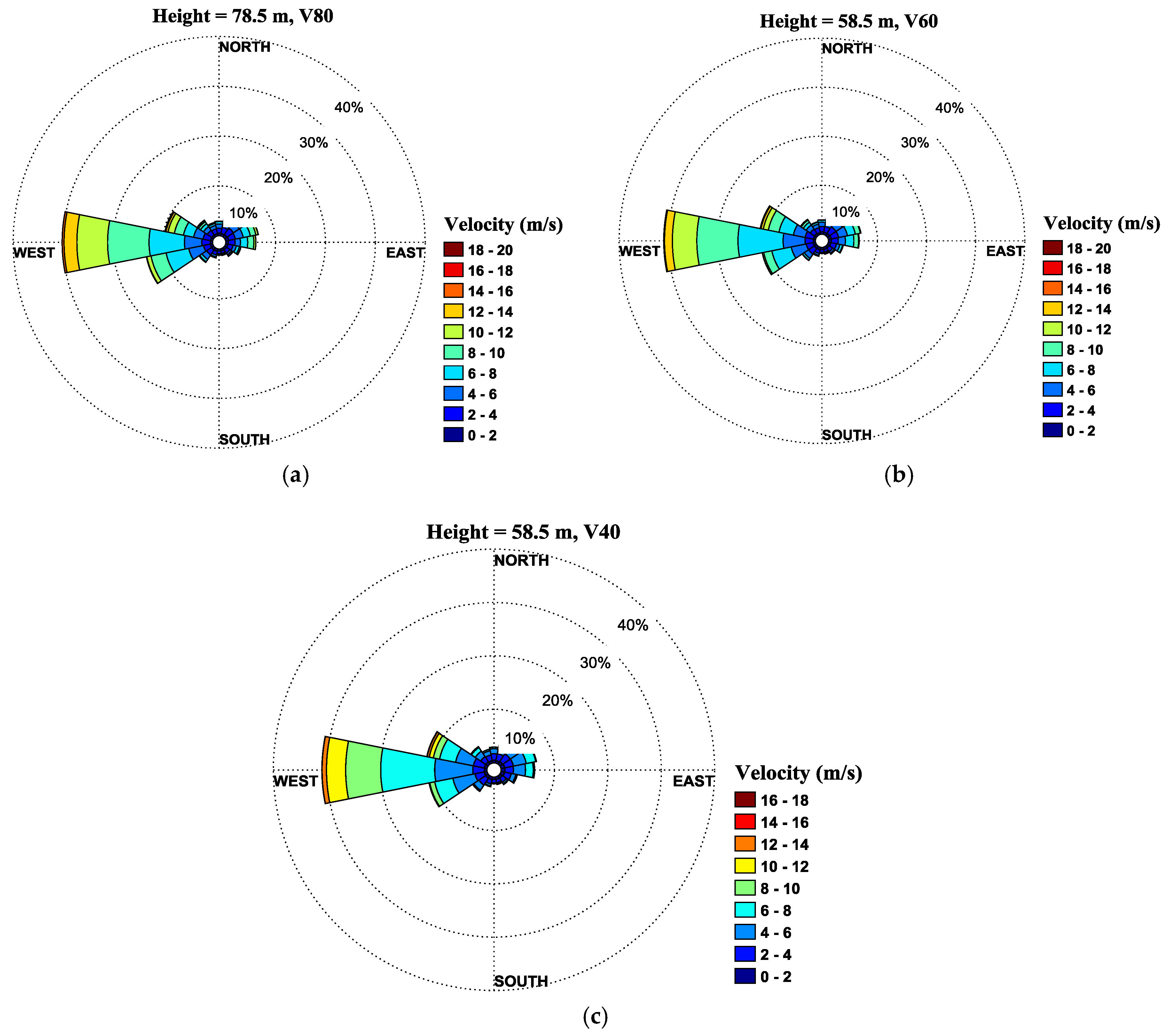
The wind rose obtained by using 10 min. average wind direction, and wind speed data at different heights is shown in Figure 10, which shows wind rose of wind velocity measured at 80 m height with wind direction obtained at 78.5 m, for wind speed at 60 m and 40 m heights versus wind direction measured at 58.5 m height. It is observed that most of the wind is from the west direction. Wind direction is calculated at 78.5 m and 58.5 m heights, respectively. At height of 80 m more than 12%, 10%, 8%, 3%, and 1% of wind is in the direction between west having wind speed ranges from 6 m/s to 8 m/s, 8 m/s to 10 m/s, 10 m/s to 12 m/s, 12 m/s to 14 m/s, and 14 m/s to 18 m/s, respectively. Similarly, the wind rose at 58.5 m height and wind speed measured at 60 m height shows 8%, 11%, 10%, 5%, 2% and 0.5% of wind speed ranges 4 m/s to 6 m/s, 6 m/s to 8 m/s, 8 m/s to 10 m/s, 10 m/s to 12 m/s, 12 m/s to 14 m/s, and 14 m/s to 16 m/s. This is ideal for a wind turbine to capture more wind to work effectively and produce more power, instead of changing direction. This also means at hub height, the wind turbine can harness more available wind power at this site. In Figure 10, wind speed frequency distribution for proposed site is shown at different heights including hub height (100 m). Wind speed frequency distribution is important to understand wind availability, through the distribution of different wind speeds by sorting into bins for a better understanding of the availability of wind speed. This helps in the good understanding of what percentage of wind speed lies most of the time. As height increases, the possibility of occurrence of a large percentage of wind speed frequencies increases. At hub height wind speed frequencies, 3 m/s to 10 m/s wind speeds lies above 8.5% each, with 7 m/s to 9 m/s in 10% each, while 11 m/s, 12 m/s and 13 m/s lies 6.2%, 4.8% and 2.8%, respectively, which is a sign of the good wind potential available at this site. At the height of 80 m, 3 m/s to 9 m/s falls above 9% each, with 6 m/s, 7 m/s and 8 m/s in 10.2%, 12% and 11.7%. While 10 m/s, 11 m/s and 12 m/s are about 7%, 5% and 3% respectively. Similarly, at height of 60 m, 3 m/s to 8 m/s wind speed lies in about 9% each, with 5 m/s, 6 m/s and 7 m/s about 11%, 12.3% and 13% each. Whereas 9 m/s, 10 m/s and 11 m/s are about 8%, 5.8% and 3% respectively. For the height of 40 m, wind speeds of 3 m/s, 4 m/s, 5 m/s, 6 m/s, 7 m/s, 8 m/s, 9 m/s, 10 m/s, 11 m/s and 12 m/s lie about 11%, 12%, 15%, 16%, 13%, 7.8%, 4.2%, 3.5%, 2.2% and 1.5%, respectively. This shows that this site is suitable for utility purpose wind power generation.
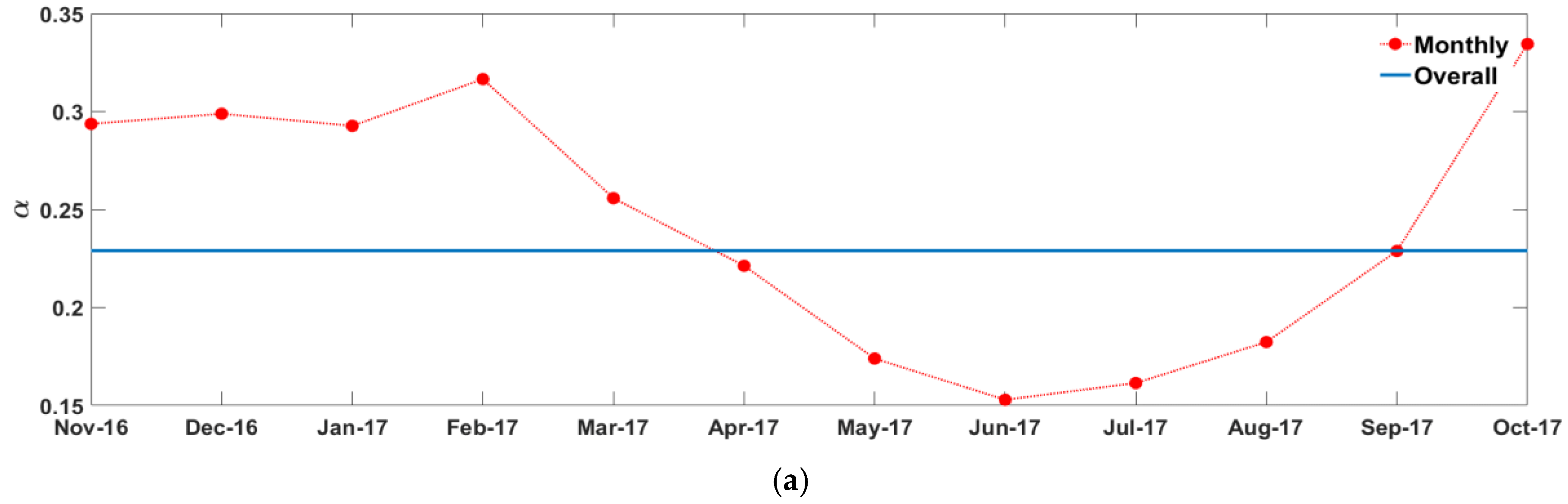
The monthly mean wind shear exponent (∝) and shear profile of this site are shown in Figure 11a,b respectively. The wind shear exponent (∝) of the power law model is analyzed for atmospheric boundary layer. It is estimated by using regression analysis using 10 min average data of wind speed sensors at heights of 80 m 60 m, and 40 m for one-year data from Nov-2016 to Oct- 2017. Alpha (∝) keeps on varying with time of the year, and its value is dependent on the site. The overall average of alpha (∝) for Sanghar is 0.229. The minimum wind shear exponent (∝) observed is 0.1528 in the month of June and maximum wind shear exponent (∝) observed is 0.3344 in the month of October.
4.4. Wind Speed Distribution and Methods
Moreover, the lowest values were observed in April, May, June, July, August, and September. In the shear profile, the wind velocities of all sensors at heights of 80 m, 60 m, and 40 m were fitted to estimate hub height velocity at 100 m. This is estimated to be 6.75 m/s as shown in Figure 12. The comparison among five Weibull methods fitting over wind speed data at each height including Vhub is shown in Figure 13. For wind speed distribution at heights of 80 m and 60 m, it can be observed that all methods fitted appropriately; however, the Graphical Method (GM) showed poor performance over the measured data. At the 40 m height, GM and MMLM almost fit the data, but EMJ, EML, and EPF have slightly differences in fitting, so MMLM is considered as the finest method for estimating wind power potential at this site. Moreover, details on the monthly and overall values of mean wind speed, shape , scale , wind power density and energy obtained by using MMLM method is shown in Table 3, where the estimated monthly mean and yearly values of wind speed, shape , scale , wind power density (W/m2) and energy density (kWh/m2) at different heights are shown. These parameters are obtained using the MMLE method for a Weibull distribution. A one-year period of data is analyzed. At hub height (100 m), the maximum mean wind speed is 9.35 m/s in June, shape parameter is 3.40 in September, scale parameter is 10.42 in June, wind power density (kW/m2) is 624.71 in June and energy density (kWh/m2) is 449.79 also in June. The overall yearly averages are 6.85 m/s, 2.46, 7.69 m/s, 323.93 (kW/m2) and 2.837 (MWh/m2). It is observed for all heights that the lowest wind characteristics occur in the month of November and highest in June.
In this research work, the authors followed the international standard, IEC 61400-12-1 in order to select the WTs to estimate the power performance of a wind turbine. Through the IEC standards, the power curve of the wind turbine is considered for calculating the annual energy production [58]. The performance of a wind turbine is indicated by the power curve. There are various methods available in the literature to develop the power curve model. In which the turbine specifications from the manufacturers and the wind speed data of a particular site are used [59,60]. Moreover, in this study, the discrete model is used. The estimation of the output power of a wind turbine is done by arranging the wind speed data of the studied site into bins and the reliable hours for every bin are collected. According to the IEC international standards, the discrete model is a simple method that does not require any mathematical functions for describing the curve [58]. The power curve of each turbine was modeled into tabular form and then the number of probable hours for each bin and corresponding power output were calculated.
The average energy generated in GWh/year by ten different turbines at four hub heights is estimated and shown in Figure 15a. The detail of wind turbine models with their characteristics is provided in Table 4. The performance of Vestas V126/3300 and Goldwind GW121/2500 outperformed the rest of turbine models at four hub heights (120 m, 100 m, 80 m, and 60 m). The estimated units generated (GWh/year) by Vestas V126/3300 and Goldwind GW121/2500 at four hub heights are 16.85 m, 15.72 m, 14.13 m, 12.56 m and 13.91 m, 13.13 m, 12 m, and 10.84 m respectively.
The capacity factor (%) of ten different turbines at four hub heights on the proposed site is calculated and revealed in Figure 15b. The capacity factor for all ten turbines is located in the appropriate range with maximum values of 63.5%, 59.9%, 54.8% and 49.5% for Goldwind GW121/2500 at four hub heights. Followed by Vestas V126/3300 and Gamesa G97/2.0, with a slight difference between both, estimated C.F is 58.3, 54.4, 48.9, 43.4 and 58.1, 54.1, 48.7, 43.3%, respectively. The lowest C.F 37.5, 33.4, 28.6 and 24.3% was estimated for the Nordex n80/2500 wind turbine at four hub heights, which is an economical range of C.F. For all turbine models, C.F. lies in the excellent range, which shows that this site has a tremendous capacity to generate electrical power for most of the available wind turbines. More details are specified in Table 5, whereas, Table 6 shows the annual values of shape (k) and scale (c) parameters obtained by EMJ, EML, EPF GM and MMLM methods at the heights of 80 m, 60 m, and 40 m. The overall results of performance evaluation of different Weibull models based on the parameters explained in Section 2.5 are compared in Table 7.
In additions, Figure 15, Table 4 and Table 5 show the units generated (GWh/year) and CF by particular wind turbines. However, the CF was estimated by the ratio of the average power output to the rated power of the generator [61]. It is used to estimate the average energy production (units generated) of a wind turbine to estimate the cost of the system [61,62,63].
5. Conclusions
In this study, different wind turbine prototype models are considered based on the wind characteristics for evaluating and investigating the wind power potential along the coastline. For this purpose, a site located in coastal zone of Pakistan is evaluated owing to its vast potential for installation of commercial wind farms. Real-time one year (Nov. 2016 to Oct. 2017) wind speed data was analyzed to estimate the twelve months mean values as well as the yearly mean at the proposed site where a wind mast had been installed and funded by the World Bank. The data was observed on the daily basis (24 h) in order to predict the behavior of wind more accurately. Based on the results, the following conclusions are obtained:
- Monthly and diurnal wind characteristics of the proposed site indicate that it has class three or higher wind potential. Therefore, according to the international standards, the proposed site is most suitable as depicted in Table 2 for wind turbine installation to supply the electricity to local communities.
- Basically, in the whole year, it is observed from the wind rose diagram, the wind directions at different heights show that most of the wind gusts blow from the west.
- The proposed site is most suitable with advantages on air density, wind shear exponent, low turbulence intensity, adequate wind speed distribution, and reliable capacity factor.
- In this research, the energy generated by ten different suggested wind turbine models indicates that the performance of two WTs such as; Vestas V126/3300 and Goldwind GW 121/2500 is better as compared to other prototypes for this proposed site.
- Also, from five Weibull distribution techniques, GM shows the inadequate performance, whereas, MMLM presents the optimum performance as compared to its counter techniques.
- The maximum values of Weibull shape and scale parameters were also calculated to understand the seasonal wind characteristics for this site. During the spring-summer seasons, the shape values are 2.60 (spring) and 3.25 (summer) respectively. Whereas, the scale values are more than 9.0 (summer) and approximately 8.2 (spring), and even better for whole of the years.
It can be noted that this site has comparatively better wind characteristics. Additionally, this study also aims to provide a policy implication for optimal selection of a suitable site, wind turbine prototype and parameters evaluation based on the real-time data assessment and analysis. It is recommended that GoP should focus on the proposed site for future economic development and electricity generation for powering local communities and underprivileged regions.
Author Contributions
D.I. supervised the project. M.H.B. and D.I. developed the idea and then requested B.A., A.A.M. and T.A.G. for Wind data collection for the study purpose at the proposed site. M.H.B. and B.A. analyzed the wind data to gather the results. B.A., A.A.M. and T.A.G. helped in responding to the reviewers’ comments. D.I. and S.T.C. helped in writing and proof reading the manuscript. However, all authors participated equally.
Funding
This research was funded by Universiti Sains Malaysia under Postdoctoral Research Fellowship Programme.
Acknowledgments
This work was supported by Universiti Sains Malaysia, and greatly acknowledged to Mehran University of Engineering and Technology and Pakistan Metrological Department.
Conflicts of Interest
The authors declare no conflict of interest.
Nomenclature
| AEDB | Alternative energy distribution board |
| CPEC | China Pakistan economic corridor |
| EPF | Energy pattern factor |
| EPM | Energy pattern method |
| EMJ | Energy pattern by Jestus |
| EML | Energy pattern by Lysen |
| FD | Frequency distribution |
| GW | Gigawatt |
| GM | Graphical method |
| IEC | International electro technical commission |
| HVDC | High voltage direct current |
| KESC | Karachi electric supply company |
| kWh | Kilowatt hour |
| kV | Kilovolts |
| LPG | Liquid petroleum gas |
| MMLM | Modified maximum likelihood method |
| MLEM | Maximum likelihood estimation method |
| MTOE | Million tons of oil equivalent |
| MW | Megawatt |
| C.F. | Capacity factor |
| MATLAB | Matrix laboratory |
| MSE | Mean squared error |
| MAE | Mean absolute error |
| NTDC | National transmission and distribution company |
| NEPRA | National electric power regulation authority |
| RI | Ruggedness index |
| RMSE | Root mean squared error |
| SP | Sheared power |
| TI | Turbulence intensity |
| TPES | Total primary energy supply |
| WPD | Wind power density |
| WR | Wind rose |
| GoP | Government of Pakistan |
| GE | General Electric |
References
- Energy (Chapter 19), 11th Five Year Plans Information Management, Ministry of Planning, Development and Reform, Pakistan. Available online: http://pc.gov.pk/uploads//plans//Ch19-Energy1.pdf (accessed on 15 July 2018).
- Hanan, I. Is it wise to compromise renewable energy future for the sake of expediency? An analysis of Pakistan’s long-term electricity generation pathways. Energy Strategy Rev. 2017, 17, 6–18. [Google Scholar]
- Yousaf, A.; Butt, M.; Sabir, M.; Mumtaz, U.; Salman, A. Selection of suitable site in Pakistan for wind power plant installation using analytic hierarchy process (AHP). J. Control Decis. 2018, 5, 117–128. [Google Scholar]
- Tauseef, A.; Shahid, M.; Bhatti, A.A.; Saleem, M.; Anandarajah, G. Energy security and renewable energy policy analysis of Pakistan. Renew. Sustain. Energy Rev. 2018, 84, 155–169. [Google Scholar]
- GhulamSarwar, K.; Wang, J.; Baloch, M.H.; Tahir, S. Wind Energy Potential at Badin and Pasni Costal Line of Pakistan. Int. J. Renew. Energy Dev. 2017, 6, 1–6. [Google Scholar]
- Baloch, M.H.; Kaloi, G.S.; Memon, Z.A. Current scenario of the wind energy in Pakistan challenges and future perspectives: A case study. Energy Rep. 2016, 2, 201–210. [Google Scholar] [CrossRef] [Green Version]
- Albani, A.; Ibrahim, M.Z. Wind Energy Potential and Power Law Indexes Assessment for Selected Near-Coastal Sites in Malaysia. Energies 2017, 10, 307. [Google Scholar] [CrossRef]
- Choi, D.G.; Min, D.; Ryu, J.-H. Economic Value Assessment and Optimal Sizing of an Energy Storage System in a Grid-Connected Wind Farm. Energies 2018, 11, 591. [Google Scholar] [CrossRef]
- Tahir, S.; Wang, J.; Baloch, M.H.; Kaloi, G.S. Digital Control Techniques Based on Voltage Source Inverters in Renewable Energy Applications: A Review. Electronics 2018, 7, 18. [Google Scholar] [CrossRef]
- The State of Industry Report 2015; Future NTDC Network; National Electric Power Regulatory Authority Islamabad, Pakistan. Available online: https://www.nepra.org.pk/Publications/State%20of%20Industry%20Reports/State%20of%20Industry%20Report%202015.pdf (accessed on 10 July 2018).
- Qamar, S.N. Alternative and Renewable Energy Policy 2011. Available online: http://climateinfo.pk/frontend/web/attachments/data-type/MoWP_AEDB%20(2011)%20Alternative%20and%20Renewable%20Energy%20Policy%20-%20Midterm%20Policy.pdf (accessed on 10 July 2018).
- Harijan, K.; Uqaili, M.A.; Memon, M.; Mirza, U.K. Forecasting the diffusion of wind power in Pakistan. Energy 2011, 36, 6068–6073. [Google Scholar] [CrossRef]
- Elliott, D. Wind Resource Assessment and Mapping for Afghanistan and Pakistan, National Renewable Energy Laboratory Golden Colorado, USA. 2007. Available online: http://www.nrel.gov/international/pdfs/afg_pak_wind_june07.pdf (accessed on 10 July 2018).
- Masseran, N. Evaluating wind power density models and their statistical properties. Energy 2015, 84, 533–541. [Google Scholar] [CrossRef]
- Ucar, A.; Balo, F. Investigation of wind characteristics and assessment of wind-generation potentiality in Uludağ-Bursa, Turkey. Appl. Energy 2009, 86, 333–339. [Google Scholar] [CrossRef]
- Celik, A.N.; Makkawi, A.; Muneer, T. Critical evaluation of wind speed frequency distribution functions. J. Renew. Sustain. Energy 2010, 2, 013102. [Google Scholar] [CrossRef]
- Gokcek, M.; Bayulken, A.; Bekdemir, S. Investigation of wind characteristics and wind energy potential in Kirklareli, Turkey. Renew. Energy 2007, 32, 1739–1752. [Google Scholar] [CrossRef]
- Tuller, S.; Brett, A. The characteristics of wind velocity that favor the fitting of a Weibull distribution in wind speed analysis. J. Appl. Meteorol. 1984, 23, 124–134. [Google Scholar] [CrossRef]
- Shu, Z.R.; Li, Q.S.; Chan, P.W. Statistical analysis of wind characteristics and wind energy potential in Hong Kong. Energy Convers. Manag. 2015, 101, 644–657. [Google Scholar] [CrossRef]
- Razavieh, A.; Sedaghat, A.; Ayodele, R.; Mostafaeipour, A. Worldwide wind energy status and the characteristics of wind energy in Iran, case study: The province of Sistan and Baluchestan. Int. J. Sustain. Energy 2014, 36, 103–123. [Google Scholar] [CrossRef]
- Ali, S.; Lee, S.M.; Jang, C.M. Statistical analysis of wind characteristics using Weibull and Rayleigh distributions in Deokjeok-do Island–Incheon, South Korea. Renew. Energy 2018, 123, 652–663. [Google Scholar] [CrossRef]
- Ali, S.; Lee, S.M.; Jang, C.M. Forecasting the Long-Term Wind Data via Measure-Correlate-Predict (MCP) Methods. Energies 2018, 11, 1541. [Google Scholar] [CrossRef]
- Baloch, M.H.; Wang, J.; Kaloi, G.S.; Memon, A.A.; Larik, A.S.; Sharma, P. Techno-Economic Analysis of Power Generation from a Potential Wind Corridor of Pakistan: An Overview. Available online: https://onlinelibrary.wiley.com/doi/full/10.1002/ep.13005 (accessed on 14 February 2019).
- Rehman, S.; Al-Abbadi, N.M. Wind shear coefficient, turbulence intensity and wind power potential assessment for Dhulom, Saudi Arabia. Renew. Energy 2008, 33, 2653–2660. [Google Scholar] [CrossRef] [Green Version]
- Wind Resource Assessment Handbook, Fundamentals for Conducting a Successful Monitoring Program; NREL Subcontract No. TAT-5-15283-01; AWS Scientific Inc.: Albany, NY, USA, 1997.
- Elosegui, U.; Egana, I.; Ulazia, A.; Ibarra-Berastegi, G. Pitch angle misalignment correction based on benchmarking and laser scanner measurement in wind farms. Energies 2018, 11, 3357. [Google Scholar] [CrossRef]
- Ulazia, A.; Saenz, J.; Berastegui, G.I. Sensitivity to the use of 3DVAR data assimilation in a meso-scale model for estimating offshore wind energy potential. A case study of the Iberian northern coastline. Appl. Energy 2016, 180, 617–627. [Google Scholar] [CrossRef]
- Saenko, A.V. Assessment of Wind Energy Resources for Residential Use in Victoria, BC, Canada. Master’s Thesis, School of Earth and Ocean Sciences, University of Victoria, Victoria, BC, Canada, 28 January 2008. [Google Scholar]
- Lima, L.D.A.; Filho, C.R.B. Wind resource evaluation in São João do Cariri (SJC)—Paraiba, Brazil. Renew. Sustain. Energy Rev. 2012, 16, 474–480. [Google Scholar] [CrossRef]
- Manwell, J.F.; McGowan, J.G.; Rogers, A.L. Wind Energy Explained: Theory, Design and Application; John Wiley & Sons: Chichester, UK, 2010. [Google Scholar]
- Katinas, V.; Marčiukaitis, M.; Gecevičius, G.; Markevičius, A. Statistical analysis of wind characteristics based on Weibull methods for estimation of power generation in Lithuania. Renew. Energy 2017, 113, 190–201. [Google Scholar] [CrossRef]
- Farrugia, R.N. The wind shear exponent in a Mediterranean island climate. Renew. Energy 2003, 28, 647–653. [Google Scholar] [CrossRef]
- Baloch, M.H.; Abro, S.A.; SarwarKaloi, G.; Mirjat, N.H.; Tahir, S.; Nadeem, M.H.; Gul, M.; Memon, Z.A.; Kumar, M. A Research on Electricity Generation from Wind Corridors of Pakistan (Two Provinces): A Technical Proposal for Remote Zones. Sustainability 2017, 9, 1611. [Google Scholar] [CrossRef]
- Elliott, D.L.; Schwartz, M.N. Wind Energy Potential in the United States. In Proceedings of the Project Energy ’93: Real Energy Technologies—Environmentally Responsible—Ready for Today, Independence, Washington, DC, USA, 21–23 June 1993. [Google Scholar]
- Yu, X.; Qu, H. Wind power in China—Opportunity goes with challenge. Renew. Sustain. Energy Rev. 2010, 14, 2232–2237. [Google Scholar] [CrossRef]
- Ilinca, A.; Mccarthy, E.; Chaumel, J.-L.; Rétiveau, J.-L. Wind potential assessment of Quebec Province. Renew. Energy 2003, 28, 1881–1897. [Google Scholar] [CrossRef]
- Zhou, W.; Yang, H.; Fang, Z. Wind power potential and characteristic analysis of the Pearl River Delta region, China. Renew. Energy 2006, 31, 739–753. [Google Scholar] [CrossRef]
- Available online: http://www.nrel.gov/gis/wind_detail.html (accessed on 30 August 2018).
- Krohn, S.; Morthorst, P.E.; Awerbuch, S. The Economics of Wind Energy; Report by European Wind Energy Association (EWEA). Available online: http://www.ewea.org/fileadmin/files/library/publications/reports/Economics_of_Wind_Energy.pdf (accessed on 30 August 2018).
- Elliott, D.L.; Schwartz, M.N. Wind Energy Potential in the United States; PNL-SA-23109, NTIS No. DE94001667; Pacific Northwest Laboratory: Richland, WA, USA, 1993. [Google Scholar]
- Li, M.; Li, X. Investigation of wind characteristics and assessment of wind energy potential for Waterloo region, Canada. Energy Convers. Manag. 2005, 46, 3014–3033. [Google Scholar] [CrossRef]
- Schwartz, M.; Elliott, D. Towards a Wind Energy Climatology at Advanced Turbine Hub Heights; NREL/CP-500-38109; National Renewable Energy Laboratory: Golden, CO, USA, 2005. [Google Scholar]
- Bianchi, F.D.; Mantz, R.J.; De Battista, H. Wind Turbine Control Systems: Principles, Modelling and Gain Scheduling Design; Springer Science & Business Media: London, UK, 2006. [Google Scholar]
- Ohunakin, O.S.; Adaramola, M.S.; Oyewola, O.M. Wind energy evaluation for electricity generation using WECS in seven selected locations in Nigeria. Appl. Energy 2011, 88, 3197–3206. [Google Scholar] [CrossRef]
- Ucar, A.; Balo, F. Evaluation of wind energy potential and electricity generation at six locations in Turkey. Appl. Energy 2009, 86, 1864–1872. [Google Scholar] [CrossRef]
- Chang, T.P. Estimation of wind energy potential using different probability density functions. Appl. Energy 2011, 88, 1848–1856. [Google Scholar] [CrossRef]
- Kwon, S.D. Uncertainty analysis of wind energy potential assessment. Appl. Energy 2010, 87, 856–865. [Google Scholar] [CrossRef]
- Costa Rocha, P.A.; de Sousa, R.C.; de Andrade, C.F.; da Silva, M.E.V. Comparison of seven numerical methods for determining Weibull parameters for wind energy generation in the northeast region of Brazil. Appl. Energy 2012, 89, 395–400. [Google Scholar] [CrossRef]
- Khahro, S.F.; Tabbassum, K.; Soomro, A.M.; Dong, L.; Liao, X. Evaluation of wind power production prospective and Weibull parameter estimation methods for Babaurband, Sindh Pakistan. Energy Convers. Manag. 2014, 78, 956–967. [Google Scholar] [CrossRef]
- Lysen, E.H. Introduction to Wind Energy; SWD 82-1; SWD: Amersfoort, The Netherlands, 1983. [Google Scholar]
- Justus, C.G.; Hargraves, R.; Mikhail, A.; Graber, D. Methods for estimating wind speed frequency distributions. J. Appl. Meteorol. 1977, 17, 350–353. [Google Scholar] [CrossRef]
- AdaramolaMuyiwa, S.; Martin Agelin-Chaab, B.; Paul Samuel, S. Assessment of wind power generation along the coast of Ghana. Energy Convers. Manag. 2014, 77, 61–69. [Google Scholar] [CrossRef]
- Chang, T.P. Performance comparison of six numerical methods in estimating Weibull parameters for wind energy application. Appl. Energy 2011, 88, 272–282. [Google Scholar] [CrossRef]
- Levent, B.; Mehmet, I.; Yılser, D.; Ayhan, A. An investigation on wind energy potential and small scale wind turbine performance at Incek region—Ankara, Turkey. Energy Convers. Manag. 2015, 103, 910–923. [Google Scholar]
- Akdag, S.A.; Dinler, A. A new method to estimate Weibull parameters for wind energy applications. Energy Convers. Manag. 2009, 50, 1761–1766. [Google Scholar] [CrossRef]
- Ulazia, A.; Ibarra, G.; Sáenz, J.; Carreno-Madinabeitia, S.; González-Rojí, S.J. Seasonal air density variations over the East of Scotland and the consequences for offshore wind energy. In Proceedings of the 7th International Conference on Renewable Energy Research and Applications, Paris, France, 14–17 Ocotber 2018. [Google Scholar]
- Ulazia, A.; Sáenz, J.; Ibarra-Berastegui, G.; González-Rojí, S.J.; Carreno-Madinabeitia, S. Using 3DVAR data assimilation to measure offshore wind energy potential at different turbine heights in the West Mediterranean. Appl. Energy 2017, 208, 1232–1245. [Google Scholar] [CrossRef] [Green Version]
- International Standard IEC 61400-12-1, Wind Turbines-Power Performance Measurement of Electricity Producing wind Turbines. Available online: ftp://ftp.ee.polyu.edu.hk/wclo/Ext/OAP/IEC61400part12_1_WindMeasurement.pdf (accessed on 10 December 2018).
- Mathew, S. Wind Energy-Fundamentals, Resource Analysis and Economics; Springer: Berlin, Germany, 2006. [Google Scholar]
- Kusiak, A.; Zheng, H.; Song, Z. Models formonitoring wind farmpower. Renew. Energy 2009, 34, 583–590. [Google Scholar] [CrossRef]
- Jowder, F.A.L. Wind power analysis and site matching of wind turbine generators in Kingdom of Bahrain. Appl. Energy 2009, 86, 538–545. [Google Scholar] [CrossRef]
- Powell, W.R. An analytical expression for the average output power of a wind machine. Sol. Energy 1981, 26, 77–80. [Google Scholar] [CrossRef]
- Chang, T.-P.; Liu, F.-J.; Ko, H.-H.; Cheng, S.-P.; Sun, L.-C.; Kuo, S.-C. Comparative analysis on power curve models of wind turbine generator in estimating capacity factor. Energy 2014, 73, 88–95. [Google Scholar] [CrossRef]
Figure 1.
Power generation capacity F.Y 2017-18.

Figure 2.
Demand and supply projection for fuels, domestic fuel production and fuel imports.

Figure 3.
Yearly demand graph of NTDC and KESC.

Figure 4.
Wind map of Pakistan showing all provinces (for interpretation of the references to color in this figure, the reader is referred to the web version of this article [13].
Figure 4.
Wind map of Pakistan showing all provinces (for interpretation of the references to color in this figure, the reader is referred to the web version of this article [13].

Figure 5.
Wind mast and its surroundings at proposed site. (Right side of figure).The complete structure of wind mast, used for collecting wind data, (top left) microscopic view of tower top, (bottom Left) Microscopic view of tower ground.
Figure 5.
Wind mast and its surroundings at proposed site. (Right side of figure).The complete structure of wind mast, used for collecting wind data, (top left) microscopic view of tower top, (bottom Left) Microscopic view of tower ground.

Figure 6.
Topographic maps for Sanghar site. (a) Elevation map 20 × 20 km (with mast in center) with 10 m elevation difference between lines. Altitudes in map range from 13 m to 25 m (warmer colors indicate higher altitudes). RIX value at mast is 0% using radius of 3500 m, steepness threshold of 30% (17°) and frequency distributed directional weight. (b) Ground roughness map 20 × 20 km (with mast in center). Background roughness length is 0.07 m, corresponding to open field with distributed rows of trees and low buildings. Roughness length for specific areas is 0.5 m for towns (rose color), 0 m for rivers (yellow color).

Figure 7.
Wind speed at 80 m, 60 m, 40 m and Vhub heights for Sanghar site. (a) Monthly average and (b) Daily diurnal.
Figure 7.
Wind speed at 80 m, 60 m, 40 m and Vhub heights for Sanghar site. (a) Monthly average and (b) Daily diurnal.

Figure 8.
Relation between monthly averages of air density and temperature for at Sanghar site.

Figure 9.
Turbulence intensities for velocities at different heights (a) 80 m (b) 60 m and (c) 40 m.
Figure 9.
Turbulence intensities for velocities at different heights (a) 80 m (b) 60 m and (c) 40 m.

Figure 10.
Wind rose for velocities (a) 80 m to the direction sensors at 78.5 m height (b) 60 m to the direction sensors at 58.5 m height and (c) 40 m to the direction sensors at 58.5 m height.
Figure 10.
Wind rose for velocities (a) 80 m to the direction sensors at 78.5 m height (b) 60 m to the direction sensors at 58.5 m height and (c) 40 m to the direction sensors at 58.5 m height.

Figure 11.
Monthly and yearly evaluation of shear exponent and shear profile for proposed site (a) monthly and overall values of alpha, (b) the Shear profile of site using power law for Sanghar site.
Figure 11.
Monthly and yearly evaluation of shear exponent and shear profile for proposed site (a) monthly and overall values of alpha, (b) the Shear profile of site using power law for Sanghar site.


Figure 12.
Comparison of placing the five different methods of Weibull probability distributions to measured data for Sanghar site (a) at 80 m height (b) at 60 m height and (c) at 40 m height.
Figure 12.
Comparison of placing the five different methods of Weibull probability distributions to measured data for Sanghar site (a) at 80 m height (b) at 60 m height and (c) at 40 m height.


Figure 13.
Wind speed distributions for Sanghar site (a) at vhub extrapolated height (b) at 80 m height (c) at 60 m height and (d) at 40 m height.
Figure 13.
Wind speed distributions for Sanghar site (a) at vhub extrapolated height (b) at 80 m height (c) at 60 m height and (d) at 40 m height.

Figure 14.
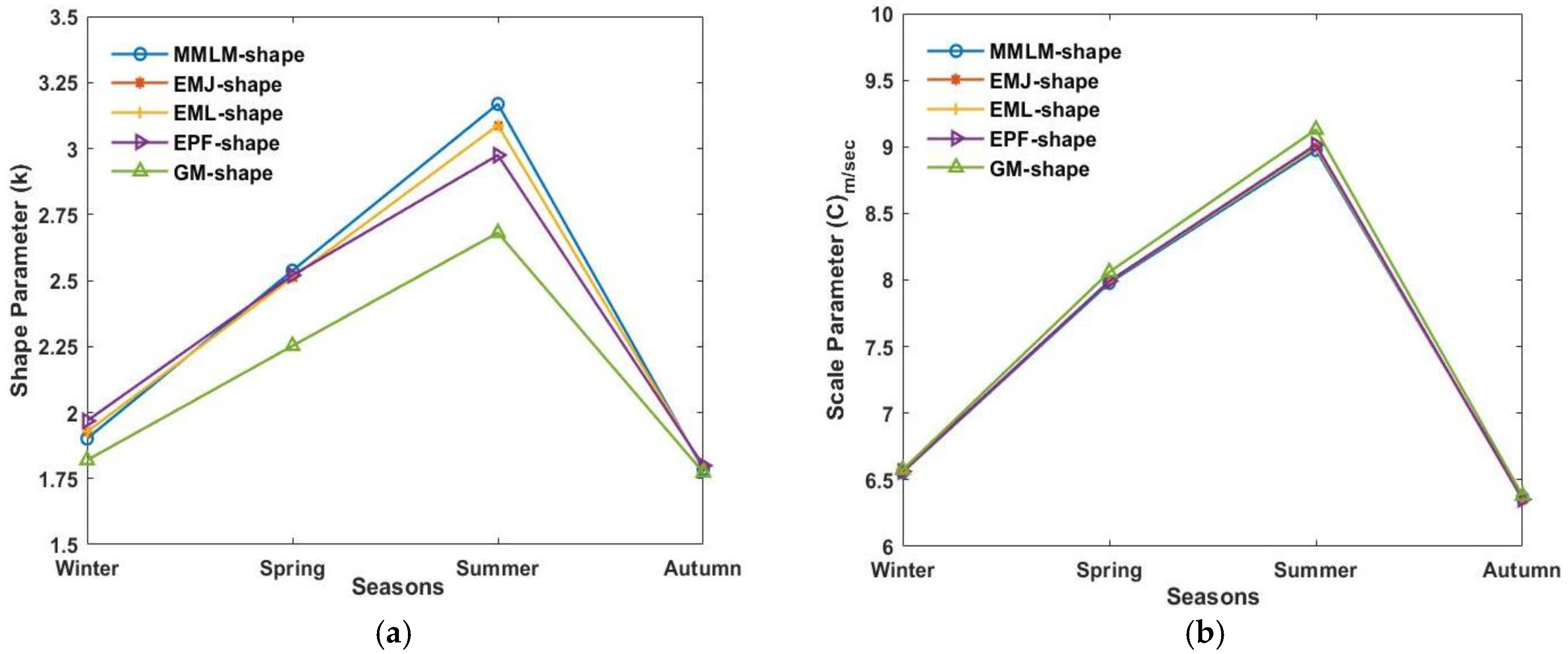
Seasonal average values of (a) the shape (k) and (b) scale (c) parameters calculated using the MMLM, EMJ, EML, EPF and GM methods.
Figure 14.
Seasonal average values of (a) the shape (k) and (b) scale (c) parameters calculated using the MMLM, EMJ, EML, EPF and GM methods.

Figure 15.
Production capacity of various wind turbine prototypes at different heights (a) the average energy generated in GWh/year and (b) a capacity factor of ten different turbines at four hub heights.
Figure 15.
Production capacity of various wind turbine prototypes at different heights (a) the average energy generated in GWh/year and (b) a capacity factor of ten different turbines at four hub heights.


Table 1.
Pakistan wind electric potential, good to excellent wind recourses at 50 m.
| Wind Resource Utility Scale | Wind Class | Wind Power W/m2 | Wind Speed m/s | Land Area km2 | Percent Windy Land | Total Capacity Installed MW |
|---|---|---|---|---|---|---|
| Good | 4 | 400–500 | 6.9–7.4 | 18,106 | 2.1 | 90,530 |
| Excellent | 5 | 500–600 | 7.4–7.8 | 5218 | 0.6 | 26,090 |
| Excellent | 6 | 600–800 | 7.8–8.6 | 2495 | 0.3 | 12,480 |
| Excellent | 7 | > 800 | > 8.6 | 543 | 0.1 | 2720 |
| Total | 26,362 | 3.1 | 131,820 |
Assumptions: Installed capacity per km2 = 5 MW; Total land area of Pakistan = 877,525 km2; The only land area included in calculations; NREL’s SARI-Energy Activities.
Table 2.
International standards of wind power generation classification at various heights.
| No. | Resourse Class | At 10 m Heights m/s W/m2 | At 30 m Heights m/s W/m2 | At 50 m Heights m/s W/m2 | |||
|---|---|---|---|---|---|---|---|
| 1 | Poor | 0–4.4 | 0–100 | 0–5.1 | 0–160 | 0–5.4 | 0–200 |
| 2 | Marginal | 4.4–5.1 | 100–150 | 5.1–5.9 | 160–240 | 5.4–6.2 | 200–300 |
| 3 | Moderate | 5.1–5.6 | 150–200 | 5.9–6.5 | 240–320 | 6.2–6.9 | 300–400 |
| 4 | Good | 5.6–6.0 | 200–250 | 6.5–7.0 | 320–400 | 6.9–7.4 | 400–500 |
| 5 | Excellent | 6.0–6.4 | 250–300 | 7.0–7.4 | 400–480 | 7.4–7.8 | 500–600 |
| 6 | Excellent | 6.4–7.0 | 300–400 | 7.4–8.2 | 480–640 | 7.8–8.6 | 600–800 |
| 7 | Excellent | >7.0 | >400 | 8.2–11 | 640–1600 | >8.6 | >800 |
Table 3.
Sanghar monthly mean and yearly wind speed.
| Parameters | 2016 | 2017 | Yearly Avg. | ||||||||||
|---|---|---|---|---|---|---|---|---|---|---|---|---|---|
| Nov | Dec | Jan | Feb | Mar | Apr | May | Jun | Jul | Aug | Sep | Oct | ||
| Vhub Height | |||||||||||||
| Vm (m/s) | 5.039 | 5.281 | 5.986 | 6.199 | 5.963 | 7.678 | 7.662 | 9.352 | 8.130 | 8.207 | 6.502 | 6.271 | 6.856 |
| k | 1.6421 | 1.7550 | 2.1115 | 1.8370 | 2.1130 | 2.3441 | 3.1549 | 3.3016 | 2.6011 | 3.3740 | 3.3963 | 1.9267 | 2.4631 |
| c (m/s) | 5.6409 | 5.9361 | 6.7593 | 6.9757 | 6.7379 | 8.6505 | 8.5472 | 10.417 | 9.1413 | 9.1140 | 7.2336 | 7.0899 | 7.6870 |
| WPD (W/m2) | 180.96 | 187.99 | 232.84 | 287.82 | 221.95 | 421.64 | 351.16 | 624.71 | 466.63 | 418.45 | 211.39 | 281.57 | 323.93 |
| E (kWh/m2) | 130.29 | 139.86 | 173.23 | 193.41 | 165.12 | 303.58 | 261.26 | 449.79 | 347.17 | 311.33 | 152.19 | 209.48 | 2836.76 |
| 80 m Height | |||||||||||||
| Vm (m/s) | 4.598 | 4.822 | 5.540 | 5.660 | 5.540 | 7.272 | 7.385 | 9.089 | 7.853 | 7.892 | 6.169 | 5.686 | 6.459 |
| k | 1.8017 | 1.8685 | 2.2450 | 1.9572 | 2.2400 | 2.3897 | 3.1657 | 3.2629 | 2.5832 | 3.3183 | 3.4982 | 2.1060 | 2.5364 |
| c (m/s) | 5.1883 | 5.4367 | 6.2585 | 6.3917 | 6.2606 | 8.1938 | 8.2377 | 10.131 | 8.8340 | 8.7752 | 6.8545 | 6.4349 | 7.2498 |
| WPD (W/m2) | 121.54 | 134.58 | 176.21 | 208.60 | 169.90 | 355.03 | 313.79 | 576.38 | 422.88 | 375.17 | 178.42 | 192.59 | 268.76 |
| E (kWh/m2) | 87.51 | 100.13 | 131.10 | 140.18 | 126.41 | 255.62 | 233.46 | 414.99 | 314.62 | 279.12 | 128.46 | 143.29 | 2354.89 |
| 60 m Height | |||||||||||||
| Vm (m/s) | 4.339 | 4.591 | 5.166 | 5.311 | 5.238 | 6.843 | 7.001 | 8.669 | 7.498 | 7.485 | 5.777 | 5.290 | 6.101 |
| k | 1.8932 | 2.0044 | 2.3782 | 2.0643 | 2.4066 | 2.4418 | 3.1812 | 3.2064 | 2.5328 | 3.2485 | 3.5554 | 2.3020 | 2.6012 |
| c (m/s) | 4.9021 | 5.1842 | 5.8279 | 6.0047 | 5.9162 | 7.7060 | 7.8062 | 9.6719 | 8.4410 | 8.3347 | 6.4135 | 5.9835 | 6.8493 |
| WPD (W/m2) | 95.63 | 108.08 | 136.23 | 164.12 | 135.96 | 291.98 | 266.27 | 503.89 | 373.08 | 323.35 | 145.42 | 143.69 | 223.97 |
| E (kWh/m2) | 68.85 | 80.41 | 101.35 | 110.29 | 101.15 | 210.23 | 198.10 | 362.80 | 277.57 | 240.58 | 104.70 | 106.90 | 1962.93 |
| 40 m Height | |||||||||||||
| Vm (m/s) | 3.836 | 4.042 | 4.533 | 4.628 | 4.676 | 6.159 | 6.428 | 8.050 | 6.933 | 6.844 | 5.173 | 4.554 | 5.488 |
| k | 2.1413 | 2.3169 | 2.6228 | 2.2715 | 2.6986 | 2.4470 | 3.1305 | 3.1047 | 2.4757 | 3.1022 | 3.5364 | 2.6969 | 2.7120 |
| c (m/s) | 4.3369 | 4.5653 | 5.1035 | 5.2295 | 5.2628 | 6.9364 | 7.1740 | 8.9964 | 7.8119 | 7.6429 | 5.7438 | 5.1286 | 6.1610 |
| WPD (W/m2) | 58.49 | 65.24 | 86.41 | 100.78 | 89.54 | 213.82 | 207.46 | 409.61 | 300.03 | 253.27 | 104.34 | 81.80 | 164.23 |
| E (kWh/m2) | 42.12 | 48.54 | 64.29 | 67.72 | 66.62 | 153.95 | 154.35 | 294.92 | 223.22 | 188.43 | 75.12 | 60.86 | 1440.14 |
The seasonal average values of the shape (k) and scale (c) parameters calculated using MMLM, EMJ, EML, EPF and GM methods at 100 m hub height for the Sanghar site, are shown in Figure 14. The shape (k) parameter calculated using MMLM, EMJ, EML, and EPF shows a small variation for all seasons, whereas the shape (k) parameter estimated by the GM method shows lower values in winter, spring and summer. The scale (c) parameter for all five methods shows closeness for all seasons with the slight increase for GM in spring and summer.
Table 4.
Wind turbine characteristics used in this study.
| Turbine Model | Rotor Diameter (m) | Swept Area (m2) | Hub Heights (m) | Rated Power (kW) | Cut-in Wind Speed (m/s) | Rated Wind Speed (m/s) | Cut-out Wind Speed (m/s) |
|---|---|---|---|---|---|---|---|
| Vestas V126/3300 | 126 | 12,469 | 166, 149, 147, 137, 117, 87 | 3300 | 3 | 12 | 22.5 |
| Goldwind GW121/2500 | 121 | 11,595 | 120, 90 | 2500 | 3 | 9.3 | 22 |
| Nordex n80/2500 | 80 | 5026 | 80, 70, 60 | 2500 | 3 | 15 | 25 |
| Nordex n90/2300 | 90 | 6362 | 105, 100, 80, 70 | 2300 | 3 | 13 | 25 |
| Suzlon S97/2100 | 97 | 7386 | 120, 90 | 2100 | 3.5 | 11 | 20 |
| Suzlon S88/2100 | 88 | 6082 | 100, 80 | 2100 | 4 | 14 | 25 |
| Gamesa G97/2000 | 97 | 7389.8 | 120, 104, 100, 90, 78 | 2000 | 3 | 19 | 25 |
| GE 1.6xle | 82.5 | 5346 | 100, 80 | 1600 | 2 | 12 | 25 |
| Nordex n60/1300 | 60 | 2828 | 69, 60, 46 | 1300 | 3 | 15 | 25 |
| Suzlon S66/1250 | 66 | 3422 | 56, 74 | 1250 | 4 | 14 | 25 |
Table 5.
Power generated, the energy produced and capacity factor of ten different turbine models.
| Turbine Model | Power Generated (kW) | Energy Produced (MWh) | Capacity Factor | Cost in Cent/kWh | Power Generated (kW) | Energy Produced (MWh) | Capacity Factor | Cost in Cent/kWh |
|---|---|---|---|---|---|---|---|---|
| Hub height | 120 m | 100 m | ||||||
| Goldwind GW121/2500 | 1588.022 | 13,911.070 | 63.52% | 3.6460 | 1498.683 | 13,128.465 | 59.95% | 3.8633 |
| Vestas V126/3300 | 1923.550 | 16,850.301 | 58.29% | 3.9732 | 1794.205 | 15,717.235 | 54.37% | 4.2596 |
| Gamesa G97/2000 | 1198.523 | 10,176.659 | 58.09% | 3.9871 | 1083.458 | 9491.095 | 54.17% | 4.2751 |
| General Electric 1.6xle | 899.114 | 7876.240 | 56.19% | 4.1213 | 833.467 | 7301.175 | 52.09% | 4.4459 |
| Suzlon S97/2100 | 1178.551 | 10,324.110 | 56.12% | 4.1267 | 1093.315 | 9577.440 | 52.06% | 4.4484 |
| Nordex n90/2300 | 1095.909 | 9600.163 | 47.65% | 4.8605 | 996.626 | 8730.443 | 43.33% | 5.3447 |
| Suzlon S88/2100 | 980.395 | 8588.260 | 46.69% | 4.9607 | 894.229 | 7833.447 | 42.58% | 5.4387 |
| Suzlon S66/1250 | 566.403 | 4961.687 | 45.31% | 5.1111 | 512.977 | 4493.677 | 41.04% | 5.6434 |
| Nordex n60/1300 | 495.826 | 4343.436 | 38.14% | 6.0721 | 443.417 | 3884.334 | 34.11% | 6.7898 |
| Nordex n80/2500 | 938.455 | 8220.869 | 37.54% | 6.1696 | 833.860 | 7304.610 | 33.35% | 6.9434 |
| Hub height | 80 m | 60 m | ||||||
| Goldwind GW121/2500 | 1369.459 | 11,996.465 | 54.78% | 4.2278 | 1237.387 | 10,839.510 | 49.50% | 4.6791 |
| Vestas V126/3300 | 1612.869 | 14,128.731 | 48.87% | 4.7385 | 1433.344 | 12,556.096 | 43.43% | 5.3320 |
| Gamesa G97/2000 | 974.237 | 8534.314 | 48.71% | 4.7544 | 865.561 | 7582.313 | 43.28% | 5.3513 |
| General Electric 1.6xle | 744.393 | 6520.880 | 46.52% | 4.9779 | 654.818 | 5736.210 | 40.93% | 5.6588 |
| Suzlon S97/2100 | 976.226 | 8551.740 | 46.49% | 4.9819 | 860.184 | 7535.210 | 40.96% | 5.6540 |
| Nordex n90/2300 | 872.157 | 7640.097 | 37.92% | 6.1075 | 754.193 | 6606.727 | 32.79% | 7.0627 |
| Suzlon S88/2100 | 784.577 | 6872.895 | 37.36% | 6.1989 | 681.072 | 5966.190 | 32.43% | 7.1409 |
| Suzlon S66/1250 | 447.351 | 3918.791 | 35.79% | 6.4713 | 385.672 | 3378.489 | 30.85% | 7.5062 |
| Nordex n60/1300 | 383.443 | 3358.965 | 29.50% | 7.8518 | 328.447 | 2877.200 | 25.27% | 9.1665 |
| Nordex n80/2500 | 714.572 | 6259.654 | 28.58% | 8.1026 | 606.776 | 5315.355 | 24.27% | 9.5420 |
Table 6.
Values of shape (k) and scale (c) Weibull parameters using five different methods.
| Methods | V80 m | V60 m | V40 m | |||
|---|---|---|---|---|---|---|
| c | k | c | k | c | k | |
| EMJ | 7.2975 | 2.2078 | 6.8927 | 2.2473 | 6.2013 | 2.258 |
| EML | 7.3005 | 2.2078 | 6.8953 | 2.2473 | 6.2035 | 2.258 |
| EPF | 7.2968 | 2.2498 | 6.892 | 2.2743 | 6.2015 | 2.249 |
| GM | 7.2952 | 2.0815 | 6.8982 | 2.1341 | 6.2028 | 2.235 |
| MMLM | 7.2938 | 2.1918 | 6.8906 | 2.2327 | 6.2033 | 2.2417 |
Table 7.
Results of performance evaluation of different Weibull models.
| Height | Model | MSE | RMSE | MAE | R | R2 |
|---|---|---|---|---|---|---|
| 80 m | MMLM | 129.30 × 10⁻⁶ | 11,371.17 × 10−6 | 7572.51 × 10−6 | 968.861 × 10⁻³ | 938.683 × 10⁻³ |
| EML | 131.66 × 10⁻⁶ | 1147.433 × 10−6 | 7573.19 × 10−6 | 968.604 × 10⁻³ | 938.194 × 10⁻³ | |
| EMJ | 132.0 × 10⁻⁶ | 1149.265 × 10−6 | 7579.21 × 10−6 | 968.533 × 10⁻³ | 938.055 × 10⁻³ | |
| EPF | 142.24 × 10⁻⁶ | 1192.628 × 10−6 | 7705.54 × 10−6 | 967.231 × 10⁻³ | 935.536 × 10⁻³ | |
| GM | 114.6 × 10⁻⁶ | 1070.514 × 10−6 | 7632.57 × 10−6 | 970.493 × 10⁻³ | 941.856 × 10⁻³ | |
| 60 m | MMLM | 110.60 × 10⁻⁶ | 1051.659 × 10−6 | 6433.59 × 10−6 | 976.764 × 10⁻³ | 954.068 × 10⁻³ |
| EML | 111.82 × 10⁻⁶ | 1057.453 × 10−6 | 6424.57 × 10−6 | 976.709 × 10⁻³ | 953.961 × 10⁻³ | |
| EMJ | 112.16 × 10⁻⁶ | 1059.078 × 10−6 | 6434.43 × 10−6 | 976.656 × 10⁻³ | 953.857 × 10⁻³ | |
| EPF | 116.30 × 10⁻⁶ | 1078.448 × 10−6 | 6452.45 × 10−6 | 976.277 × 10⁻³ | 953.116 × 10⁻³ | |
| GM | 103.94 × 10⁻⁶ | 1019.515 × 10−6 | 6512.05 × 10−6 | 977.039 × 10⁻³ | 954.607 × 10⁻³ | |
| 40 m | MMLM | 82.44 × 10⁻⁶ | 9079.72 × 10−6 | 5590.02 × 10−6 | 985.959 × 10⁻³ | 972.115 × 10⁻³ |
| EML | 81.65 × 10⁻⁶ | 9036.26 × 10−6 | 5669.49 × 10−6 | 986.139 × 10⁻³ | 972.472 × 10⁻³ | |
| EMJ | 81.74 × 10⁻⁶ | 9041.08 × 10−6 | 5671.73 × 10−6 | 986.129 × 10⁻³ | 972.451 × 10⁻³ | |
| EPF | 82.12 × 10⁻⁶ | 9061.97 × 10−6 | 5628.14 × 10−6 | 986.036 × 10⁻³ | 972.266 × 10⁻³ | |
| GM | 82.88 × 10⁻⁶ | 9103.91 × 10−6 | 5557.66 × 10−6 | 985.871 × 10⁻³ | 971.941 × 10⁻³ |
© 2019 by the authors. Licensee MDPI, Basel, Switzerland. This article is an open access article distributed under the terms and conditions of the Creative Commons Attribution (CC BY) license (http://creativecommons.org/licenses/by/4.0/).
Share and Cite
MDPI and ACS Style
Hussain Baloch, M.; Ishak, D.; Tahir Chaudary, S.; Ali, B.; Asghar Memon, A.; Ahmed Jumani, T. Wind Power Integration: An Experimental Investigation for Powering Local Communities. Energies 2019, 12, 621. https://doi.org/10.3390/en12040621
AMA Style
Hussain Baloch M, Ishak D, Tahir Chaudary S, Ali B, Asghar Memon A, Ahmed Jumani T. Wind Power Integration: An Experimental Investigation for Powering Local Communities. Energies. 2019; 12(4):621. https://doi.org/10.3390/en12040621
Chicago/Turabian StyleHussain Baloch, Mazhar, Dahaman Ishak, Sohaib Tahir Chaudary, Baqir Ali, Ali Asghar Memon, and Touqeer Ahmed Jumani. 2019. "Wind Power Integration: An Experimental Investigation for Powering Local Communities" Energies 12, no. 4: 621. https://doi.org/10.3390/en12040621
Note that from the first issue of 2016, this journal uses article numbers instead of page numbers. See further details here.