Article

Evaluation of the Complexity, Controllability and Observability of Heat Exchanger Networks Based on Structural Analysis of Network Representations

by
Daniel Leitold
1,2,
Agnes Vathy-Fogarassy
1,2 and
Janos Abonyi
2,*
1
Department of Computer Science and Systems Technology, University of Pannonia, Egyetem u. 10, H-8200 Veszprém, Hungary
2
MTA-PE Lendület Complex Systems Monitoring Research Group, University of Pannonia, Egyetem u. 10., POB. 158, H-8200 Veszprém, Hungary
*
Author to whom correspondence should be addressed.
Energies 2019, 12(3), 513; https://doi.org/10.3390/en12030513
Submission received: 25 December 2018 / Revised: 31 January 2019 / Accepted: 2 February 2019 / Published: 6 February 2019

Abstract

:
The design and retrofit of Heat Exchanger Networks (HENs) can be based on several objectives and optimisation algorithms. As each method results in an individual network topology that has a significant effect on the operability of the system, control-relevant HEN design and analysis are becoming more and more essential tasks. This work proposes a network science-based analysis tool for the qualification of controllability and observability of HENs. With the proposed methodology, the main characteristics of HEN design methods are determined, the effect of structural properties of HENs on their dynamical behaviour revealed, and the potentials of the network-based HEN representations discussed. Our findings are based on the systematic analysis of almost 50 benchmark problems related to 20 different design methodologies.
PACS:
02.30.Yy; 02.40.Pc; 02.40.Re; 02.50.Sk; 89.20.Ff; 89.75.-k; 89.75.Da; 89.75.Fb; 89.75.Hc; 89.75.Kd
MSC:
93B07; 93B51

1. Introduction

More now than ever, industrial processes are integrated to increase efficiency [1]. Process integration (PI) dates back to 1970 when PI was the response to the oil crisis, and, since then, this field has been a hot topic as it can be utilised to minimise energy and water usage [2], waste as well as emissions [3]. Since then, tools developed for Heat and Energy Integration have become essential elements of Process Design [4], including Energy Storage Systems [5]. Meanwhile, PI increases the efficiency of the technologies, and the increased complexity also complicates operations. Heat Integration also often results in more complex but less operable technologies [6]. Thus, a methodology to support the integrated system design must have a good qualitative and quantitative model that highlights the characteristics of the processes [7].
Although many works deal with the controllability [8] and observability [9] of complex systems, the connection between the complexity of the system and the difficulty of operations has not been examined in details. However, the analysis of the structural motifs of the building elements of complex systems and their models can highlight potentially useful information that can support the design and operation. The structure-relevant analysis of Heat Exchanger Networks (HENs) has already been proven to be beneficial, e.g., the resilience index (RI) quantifies the ability of a HEN to deal with disturbances [10], the controllability index measures the controllability of the HENs [11], and structural analysis can be applied to determine the locations of additional sensors that can reveal otherwise indistinguishable faults [12].
The connection between the structural properties of HENs designed by different methodologies and the operability of the system has yet to be examined in details. The optimisation of HENs can be formalised in several ways. Algorithms can focus on the minimum number of matches [13], the Maximum Energy Recovery (MER) [14], the Minimum Energy-Capital cost [15], the minimum Total Annualised Cost (TAC) [16], the minimum number of exchangers [17], or, in the case of retrofit design, the minimum number of additional exchangers and the additional area of the exchangers or piping costs [18]. The goals listed above can be achieved by different algorithms, such as the Pinch methodology [19], dual-temperature approach method [20], pseudo-pinch [21], Supertargeting [14], State-Space approach [16], branch- and bound-based algorithms [22], or the application of Genetic Algorithm and Simulated Annealing (GA and SA, respectively) [23].
Although there are no systematic studies related to how optimisation algorithms affect the structural properties of HENs with regard to operability, there are some well-known relations. The pinch methodology determines the minimum temperature difference, Δ T m i n , which divides the HEN into two sub-networks: above the Pinch and below the pinch [19]. The method enables an MER design to be created, i.e., it minimises the energy required. The price of the MER design is the increased number/area and installation costs of heat exchangers. In contrast, optimisation based on the minimum number of matches decreases the number of heat exchangers in addition to the installation cost [24], and makes the operation easier [17]. As this approach has a negative impact on TAC and utility costs, other approaches aim to minimise them [25]. The tradeoff between the targets is continuously changing from one study to the next, and it is unequivocal that the tradeoff has a significant effect on the structure of the designed HEN, along with the controllability and observability of the system.
The dynamical characteristics of the HENs have increasingly become the focus of attention, such as controllability [26,27], observability [28], flexibility [29] or operability [30,31]. The trends mentioned above highlight that it is more critical to automatically qualify the operability-related dynamical properties of HENs based on structural information. For this purpose, HENs can be transformed into the networks of state variables [32], streams and matches [33], or networks of state-space representations [34].
Over the last five years, the system analysis based on the network has spread quickly, as the number and location of necessary actuators [8] and sensors [9] can be determined efficiently by utilising the structure-based maximum matching algorithm. The maximum matching algorithm is a hot topic in other fields such as pattern recognition [35] or machine vision [36] and method to determine maximum matching in large graphs also proposed [37]. The maximum matching algorithm is widely applied also in the fields of pattern recognition [35], machine vision [36], and it can scale up to handle large graphs [37]. With this methodology, the systems are analysed in terms of how does the correlation degree affect the controllability [38], robustness [39] and energy demand [40]. How structural motifs in the network influence the controllability of a transcription network [41], a human protein-protein interaction network [42] or cancer metabolic networks [43] has also been studied.
These promising applications suggest that it could be beneficial to utilise this methodology to reveal the effect of the complexity of HENs in terms of their operability and to address the question concerning what kind of measures of network science can be applied to compare the complexity of HENs obtained by different design methodologies.
Section 2 presents three different network-based representations of HENs to explore motifs that have a significant effect on structural controllability and observability. To evaluate the structural controllability and observability of HENs, the minimum sets of driver and sensor nodes were generated. Additionally, an extended and more exhaustive version of the maximum matching-based approach was used [8] since it can underestimate the number of controllers required [44]. The generated set of driver nodes Was evaluated structurally through the number and location of driver nodes to determine control-relevant installation costs. The relative degree of the resulting dynamical system was also analysed to assess the sluggishness [45] and difficulty of the operation. A new methodology to decrease the relative degree is introduced in Section 2. Section 3 presents how the proposed approach can be used in the systematic analysis of almost 50 HEN design problems and how the developed measures can be used to compare different design methodologies.

2. Network-Based Evaluation of the Complexity, Controllability and Observability of HENs

The workflow of the proposed method is depicted in Figure 1. The method handles several goal-oriented representations of HENs to analyse their specific properties. As this work focuses on graph-based approaches, approaches based on temperature-enthalpy, heat-content or temperature-interval diagrams [46] are not discussed. As our goal was to study dynamic structural characteristics, this section presents the three most relevant models that can be used for such a purpose. After the introduction of the network-based representations, the systematic analysis of the extracted network is presented (see Figure 1). For this purpose, a MATLAB toolbox was developed, which is available at www.abonyilab.com.

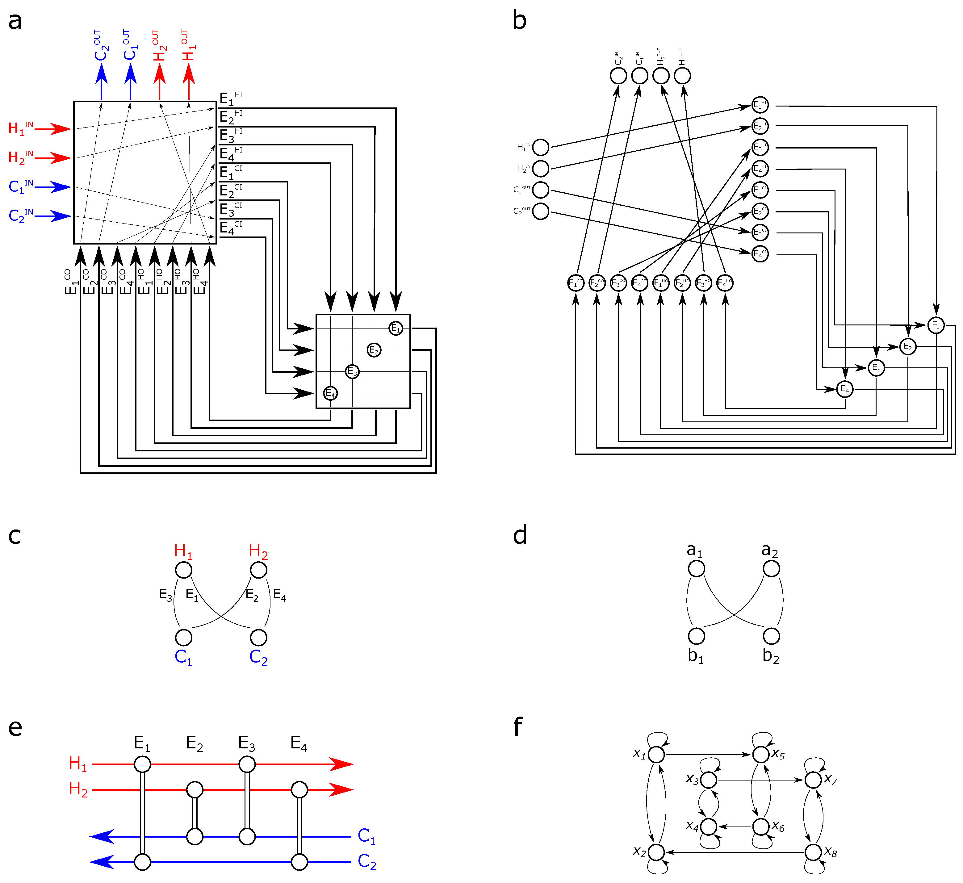
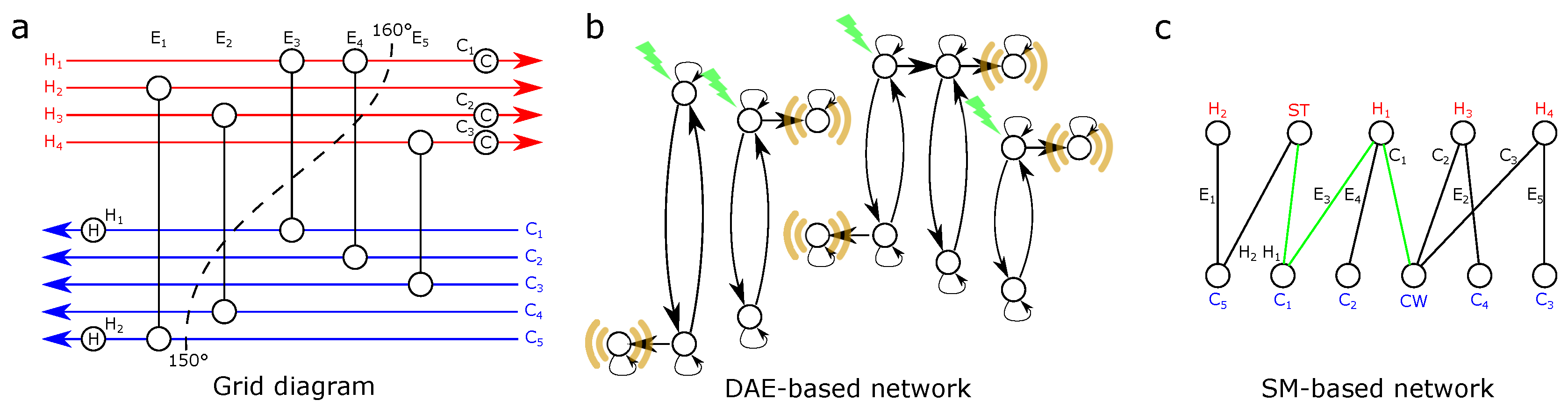
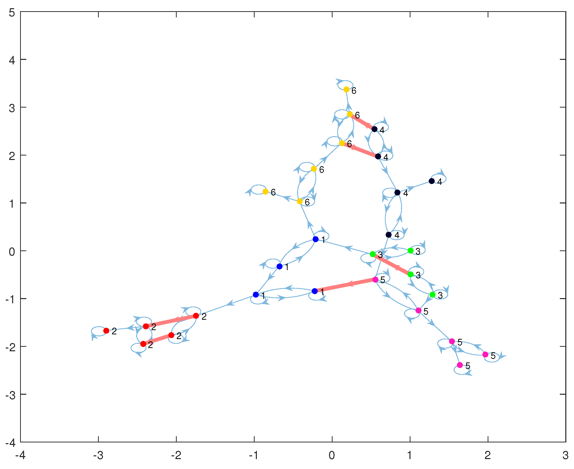
2.1. Network Representations of HENs

Besides the widely applied Process Flow Diagrams (PFDs), HENs of hot and cold streams are represented in three different ways, as illustrated in Figure 2.
The first classical representation is the state-space (SS) approach (Figure 2a), which consists of the Distribution Network (DN) and the superstructure operator [34]. The DN determines how units are located on the streams, while the superstructure operator shows the interactions between the streams. The SS-based network representation (Figure 2b) can be defined as G S S ( V S S , E S S ) based on the V S S set of vertices that contain the inlet and outlet of the streams and the E S S edges that present the connections between the heat exchangers.
The second classical representation shows how streams are matched according to the units, namely heat exchangers, utility heaters and utility coolers (Figure 2c) [33]. The second SM-based network representation is almost the same as the classical one (Figure 2d), and it can be defined as G S M ( V S M , E S M ) , where the nodes ( V S M = { V h s , V c s , V h p , V c w } ) denote the sets of hot streams ( V h s )d an cold streams ( V c s ), the high pressure steam ( V h p ) and the cold water ( V c w ). The edges ( E S M = { E h e , E u h , E u c } V S M × V S M ) represent the heat exchangers ( E h e V h s × V c s ), the utility heaters ( E u h V h p × V c s ) and the utility coolers ( E u c V h s × V c w ). The two partitions of the nodes are the hot streams (Process and utility, { V h s V h p } ) and the cold streams (Process and utility, { V c s V c w } ). The weights of the nodes represent the heat capacity of the streams, while the weights of the edges represent the heat load on the units.
The third and most common classical representation of a HEN is the Grid diagram (GD) [6,47], where the streams are presented as they are connected through the heat exchangers and influenced by utility units (Figure 2e). The dynamics of the units, i.e., the heat exchangers, utility coolers and utility heaters can be described by a differential-algebraic system of equations (DAE) as [48]:
d T h o d t = v h V h ( T h i T h o ) + U A c p h ρ h V h ( T c o T h o ) ,
d T c o d t = v c V c ( T c i T c o ) + U A c p c ρ c V c ( T h o T c o ) ,
where T h i , T c i , T h o and T c o denote the temperatures of the hot input, cold input, hot output and cold output streams, respectively; v h and v c represent the flow rates of the cold and hot streams; V h and V c stand for the volumes of the hot and cold side tanks of the heat exchanger; U is the heat transfer coefficient; A denotes the heat transfer area of the heat exchanger; and c p and ρ are the specific heat and density of the streams.
In the above representation, the state variables are the temperatures of the outlet streams of the heat exchanger x ( t ) = [ T h o , T c o ] T , the temperature of the inlet streams are regarded as disturbances d ( t ) = [ T h i , T c i ] T , and v c ( t ) and v h ( t ) are time-varying parameters [48]. The dynamics of the utility units are similar. Utility coolers can be described by Equation (1) by considering the temperature of the cold water stream T c o as a controlled input variable. Analogously, utility heaters are modeled by Equation (2) where T h o denotes the controlled inputs. HENs based on these building blocks can be represented by linear state-space models in the general form of Equations (3) and (4).
x ˙ = A x + B u + Γ d
y = C x + D u
Recently, Liu et al. introduced a network science-based representation of dynamical systems and a methodology to determine the minimal input configuration that ensures the controllability of the system [8]. The third, state-space model-based network representation (Figure 2f) easily lends itself to the application of this methodology. The resultant network can be described as a graph G D A E = ( V D A E , E D A E ) , where vertices represent the state variables x , while the edges are derived from the structure matrix of the state-transition matrix A as if A i j 0 , then an edge from x j to x i exists. As a result of Equations (1) and (2), the simplest building blocks of HENs can be defined as the heat exchanger cells, the utility coolers and the utility heaters. Their grid diagram and state-space-based network representations can be seen in Figure 3.
The SS-based network representation can be easily applied to HENs even when the streams are mixed and split. In the other two network representations, the handling of mixers and bypasses is less straightforward.
The number of vertices and edges of the SM-based network representation directly represents the streams and units, respectively. Loops and paths can be identified more easily in this network representation than in any other representations. This property is essential when the goal is not the MER design but to minimise the number of units that can be readily determined by the equation U u n = N s + L S , where U u n denotes the number of units, N s the number of streams ( | V G D | ), L the number of independent loops and S the number of separate components in the network [33]. Loops and paths should be excluded from the designs, where the target is to minimise the number of units. The presence of splitters and mixers does not influence the property U u n = N s + L S when Pinch Partitioning is excluded [49]. Furthermore, with this representation the degree of freedom of the heat loads can also be determined as H N s + S , where H denotes the number of heat exchangers ( | E h e | ) in the network.
The DAE-based network representation is suitable to analyse the operability of HENs. A system is controllable if it can be derived from an initial state to any desired final state over a finite period of time, while it is observable if any of the internal states can be reproduced by the knowledge of the initial state in addition to all the inputs and outputs [50]. The system is structurally controllable (observable) if the controllability (or observability) matrix, C = [ B , AB , , A n 1 B ] (or O = [ C T , ( CA ) T , , ( CA n 1 ) T ] T ) is of full rank, r a n k ( C ) = n (or r a n k ( O ) = n ) [51].
Liu et al. utilised the maximum matching algorithm on the DAE-based network representation to determine the minimum number of actuators (or sensors) and create a controllable (or observable) input (or output) configuration [8]. Nevertheless, how the network is represented is critical. If the adjacency matrix of the network is identical to the structure matrix of the state-transition matrix of the linear dynamical equation seen in Equation (3), then observability can be analysed, while in the reversed direction the controllability of the system can be investigated.
As each motif in the DAE-based network representation possesses a self-loop (coloured in red in Figure 3), i.e., the diagonal elements are non-zero values in the state-transition matrix, maximum matching selects these edges and leaves no unmatched node that can be a driver (or sensor) node. Since each HEN is constructed from these motifs, the approach is unusable in the case of HENs. Nevertheless, this method can be extended to be suitable for dynamical systems that exhibit this kind of behaviour. This method is referred to as the path-finding method [44] as it is also based on maximum matching, but following the maximum matching it searches for circles which can be cut off into Hamiltonian paths.
Since only the DAE network representation is detailed enough to determine the location of actuators and sensors, the relative degree can only be interpreted by this representation. To evaluate the “physical closeness” or “direct effect” of the control configuration of a nonlinear system with state equation x ˙ = f ( x ) + j = 1 m g j ( x ) u j + κ = 1 p w κ ( x ) d κ and output equation y i = h i ( x ) , relative order is introduced as a structural measure of the initial sluggishness of the response [45]. The relative degree can be determined by the standard Lie derivative. Therefore, for scalar field h i ( x ) and vector field f ( x ) it is defined as L f h i ( x ) = l = 1 n ( h ( x ) / x l ) f l ( x ) ) , where f l ( x ) denotes the row element l of f ( x ) . Higher order Lie derivatives are defined as L f k h i ( x ) = L f L f k 1 h i ( x ) , while mixed Lie derivatives L g j L f k 1 h i ( x ) in an obvious way [45]. Then, relative degree r i is defined for output y i as the smallest integer for which [ L g 1 L f r i 1 h i ( x ) L g m L f r i 1 h i ( x ) ] [ 0 0 ] with respect to input vector u if exists, otherwise r i = . The relative order r i j of output y i with respect to input u j is the smallest integer for which L g j L f r i j 1 h i ( x ) 0 if exists, otherwise r i j = . The relationship between r i and r i j can be defined as r i = m i n ( r i 1 , r i 2 , , r i m ) . Analogously to r i j , the relative order ρ i κ of output y i with respect to disturbance d κ can be defined as the smallest integer L w κ L f ρ i κ h i ( x ) 0 if exists, otherwise ρ i κ = . For linear systems that are defined above, r i j can be defined as the smallest integer for which c i A r i j 1 b j 0 , where c i is row i of C and b j is column j of B . The relative order ρ i κ with respect to the disturbance d is the smallest integer for which c i A ρ i κ 1 γ κ 0 , where γ κ denotes column κ of Γ . By utilizing the DAE network representation, the relative degree r i j can be defined as the shortest path i j from input u j to output y i minus one, r i j = i j 1 . Analogously, the relative degree ρ i κ can be defined as the geodesic path i κ from disturbance d κ to output y i minus one ( ρ i κ = i κ 1 ). The visual representation of the relative degree can be seen in Figure 4.
As can be seen in Figure 4, the shaded area represents clusters of state variables that can be achieved by a relative degree that is smaller than r i . The operability of HENs can be improved by minimising the highest relative degree with the addition of actuators or sensors [52] as will be presented in the following subsection.
The analysis of the previously introduced network representations can highlight the structural properties of HENs. The developed network-based measures are summarised in Table 1 and Table 2.

2.2. Operability-Focused Sensor and Controller Placement in HENs

Two methods are used to extend the minimal input and output configurations [58]. The first approach utilises the set-covering method. Firstly, the allowed maximal relative degree r m a x is defined. Secondly, the set of nodes W i reachable from node i over a maximum of r m a x steps was determined. In the formulation of the algorithm, U denotes the set of all the state variables, C the set of the actuators necessary to ensure structural controllability, and O the set of sensors necessary for structural observability. In the case of input (or output) configuration, J represents the set of necessary driver (or sensor) nodes, such that P is the set of state variables that is covered by J, namely P = j J W j . The goal is to minimise J such that P = U and C J (or O J ); moreover, r u r m a x , and u U . When initial input or output configurations are not given, then the method yields a global optimum for the problem. A greedy algorithm was applied to solve the set-covering problem [59].
The second approach uses two network-specific measures, namely the closeness and the node betweenness centrality measures. The closeness centrality of node i can be calculated using Equation (5).
C c ( i ) = N 1 j i i , j
Betweenness centrality calculates the number of geodesic paths that intercept node i ( σ s t ( i ) ) and divides this by the number of all the geodesic paths ( σ s t ) for each start s and target t node, such that s i t . The betweenness centrality of node i is shown in Equation (6).
B c ( i ) = s i t σ s t ( i ) σ s t
For each component that exceeds r m a x , a node with the highest centrality measure is selected as an additional actuator (or sensor), i.e., C = C { i : max ( C c ( i ) B c ( i ) ) , i C } in the case of the input configuration and O = O { i : max ( C c ( i ) B c ( i ) ) , i O } in the case of the output configuration. The steps are repeated iteratively until all the components exhibit an order not in excessive of r m a x .
For all HENs presented, the number of additional actuators and sensors required to manage the system with r m a x was calculated by the set-covering method (global optimum), the retrofit set-covering method (using existing configurations) and the retrofit centrality-based method (using current configurations). In this analysis, the maximal order was determined as r m a x = d m a x / 4 , where d m a x denotes the diameter of the network.

3. Systematic Analysis of HENs

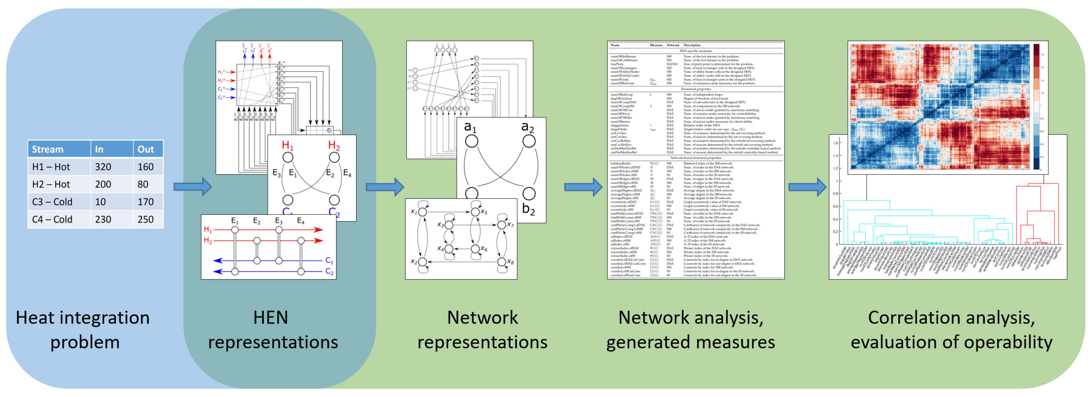
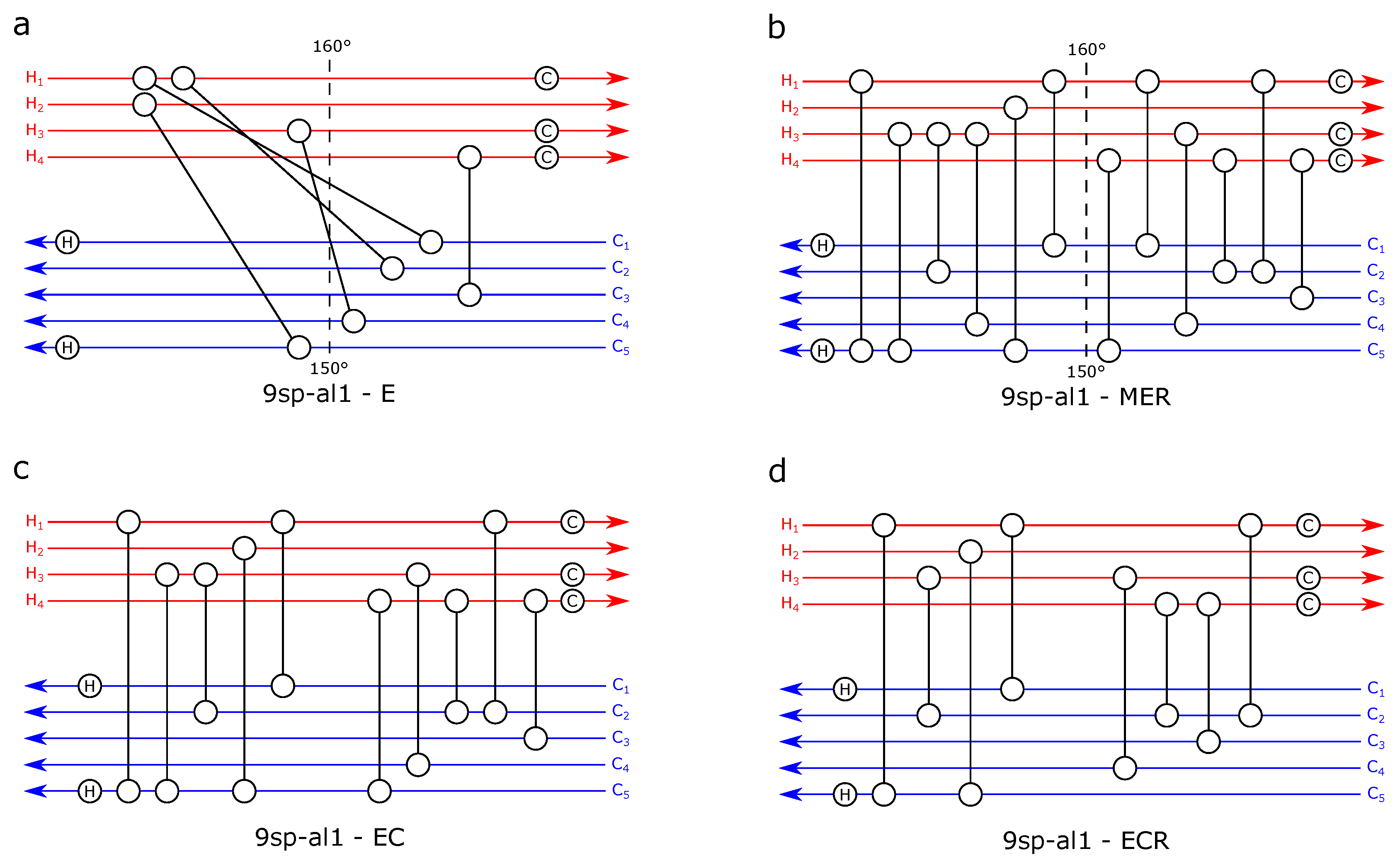
3.1. The Studied Benchmark Problems

The well-known benchmark sets of Furman and Sahinidis (2004) [60], Chen et al. (2015) [61,62] and Grossmann (2017) [63] were used to study how the proposed measures can be used to evaluate HENs and compare different design methodologies of HENs. The benchmark problems and the applied methods are summarised in Table 3, while the notation of the utilised methods and their objective functions are shown in Table 4. These problem sets contain 48 problems and 23 methods, as well as 639 different HENs, of which 539 are unique. Fifty-three different measures, as summarised in Table 5, were generated for all the HENs.

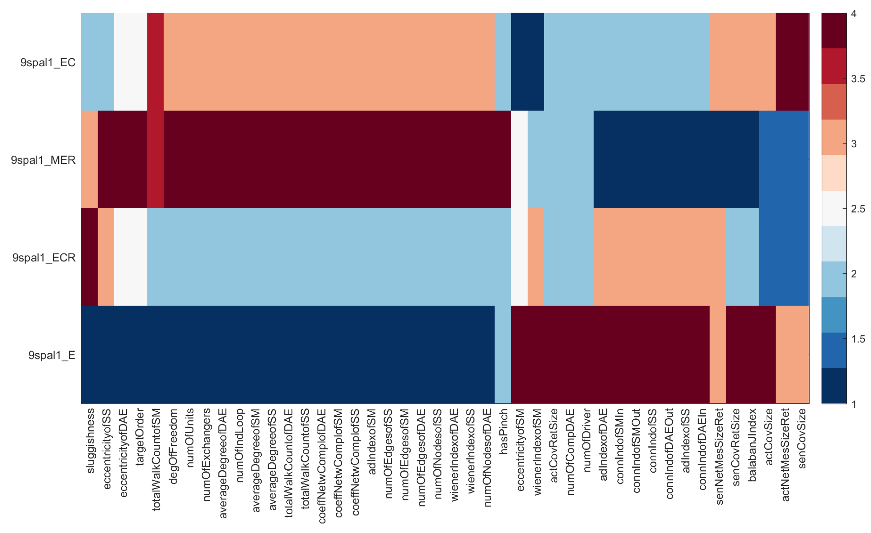
3.2. Analysis of the 9sp-al1 Problem

The 9sp-al1 benchmark problem was studied in detail to demonstrate the applicability of the proposed methodology. As can be seen in Figure 5, the solutions to the problem generated by the E, MER, EC and ECR methods significantly differed [14]. The first two solutions were based on the pinch point analysis to ensure Minimal Energy Requirement design, while the second two solutions were obtained by minimising energy and capital costs in the case of a new (EC) and retrofit (ECR) design.
The networks extracted from the HEN 9sp-al1-E solution (Figure 5a) can be seen in Figure 6. In DAE-based network representation (Figure 6b), the driver and sensor nodes are denoted by green- and orange-coloured symbols, respectively, while in SM-based network representation, a critical path is denoted by the colour green (Figure 6c).
The clusters (communities) in the DAE-based network representation were also analysed by community detection algorithms [75]. The clusters of the HEN 9sp-al1-MER can be seen in Figure 7. Such clustering of the network can highlight useful information, e.g., it can show how the HEN is integrated and how the pinch isolates the clusters.
All measures introduced in Table 5 were calculated for the presented HENs, and the results of the analysis are presented in Table 6.
As our analysis also aimed to identify structural parameters that have an impact on the dynamical properties of the HEN, firstly, the correlation between the proposed measures in these four examples was studied (see Figure 8). The results are discussed in the following section together with the analysis of all 639 HENs.

3.3. Results and Discussion of Systematic Correlation Analysis

Figure 9 shows the similarity-based ordering of the 539 unique networks (on the rows) and the measures (on the columns). The colours of the map represent rankings of the networks based on the given measures. As can be seen, the map is clustered and on the right-hand side measures that are negatively correlated to the measures on the left-hand side are presented. This phenomenon originates from the calculation of the measures (some of these are calculated mostly as the reciprocal of the measures on the left-hand side). The similarities between the most important measures are visualised by a dendrogram in Figure 10.
Based on the analysis of the results, the following conclusions can be made:
Firstly, it is visible that the studied HENs were clustered and the members of such clusters exhibited similar dynamical properties. To confirm this, the Spearman distance for each network based on the measures was generated and visualised on a heat map, as can be seen in Figure 11. On the heat map, three groups can be easily distinguished, and these groups consisted mostly of problems similar in size.
Secondly, the number of unmatched nodes that were generated by maximum matching was equal to zero for all HENs. This was caused by the SCCs and the intrinsic dynamics introduced in Figure 3. Thus, additional driver and sensor nodes should be determined by methods such as path-finding [44].
Thirdly, the number of the additional driver and sensor nodes correlated with the number of components in DAE-based representation, i.e., the number of sub-networks in the HEN. Thus, more interconnected streams demanded fewer driver and sensor nodes.
Fourthly, a smaller number of driver and sensor nodes resulted in an increased relative order, thus more complex operability.
Fifthly, the number of independent loops in the SM-based network representation correlated with the number of units in the HEN, and the average degree in SS- and SM-based network representations. The number of loops also correlated negatively with connectivity indexes. As the number of independent loops resulted in enhanced heat recovery, it attracted an increase in the number of heat exchangers too. Thus, a larger average degree meant that energy integration was greater, and more heat exchangers were utilised.
Finally, the comparison of the proposed methods showed that the results significantly varied from problem to problem. Only one correlation could be determined: the CRR, LHM and LRR algorithms solved the problem using more exchangers than other methods.

4. Conclusions

A network science-based analytical approach is proposed for the structural analysis of heat exchanger networks.
The proposed methodology utilises three different network-based representations that highlight various aspects of the dynamics of the HEN. The extracted networks were analysed by the toolbox of network science to create structural operability and complexity measures.
The analysis of more than 600 HENs confirmed that the proposed approach can be efficiently applied to the fast screening of HENs based on their structural properties.
A significant result of the analysis is that the popular maximum matching-based method used to determine the sensor and driver nodes in dynamical systems was not suitable for heat exchanger networks due to the intrinsic dynamics. It was highlighted that, with the more interconnected the HENs, fewer actuators and sensors are needed to ensure structural controllability and observability, which results in a higher relative order and the increased difficulty of the operability.
It was also highlighted that the degree-based structural measures can refer to the level of Heat Integration. The methodology was suitable for classifying the different methods that grant the HEN, as some techniques tended to determine more units in the network than others.
Although the proposed methodology has been introduced for the analysis of HENs, it can be applied to a broader class of dynamical systems. In our further research, we will generalise the results by examining the integrated and multi-objective design of processes and their control systems and studying the network topology-based properties of dynamical systems.

Author Contributions

D.L. reviewed the literature on network science and heat exchanger networks, developed the algorithms, designed and performed the experiments, and wrote the related sections. A.V.-F. participated in the formalisation of the methodology. J.A. conceived and designed the core concept, developed the algorithms and proofread the paper.

Funding

This research was supported by the National Research, Development and Innovation Office NKFIH, through the project OTKA-116674 (Process mining and deep learning in the natural sciences and process development) and the EFOP-3.6.1- 16-2016- 00015 Smart Specialization Strategy (S3) Comprehensive Institutional Development Program. Daniel Leitold was supported by the ÚNKP-18-3 New National Excellence Program of the Ministry of Human Capacities.

Conflicts of Interest

The authors declare no conflicts of interest. The founding sponsors had no role in the design of the study; in the collection, analyses, or interpretation of data; in the writing of the manuscript; nor in the decision to publish the results.

Abbreviations

CNCCoefficient of Network Complexity
DAEDifferential Algebraic Equations
DNDistribution Network
GAGenetic Algorithm
GDGrid Diagram
HENHeat Exchanger Network
MERMaximum Energy Recovery or Minimum Energy Requirement
PIProcess Integration
PFDProcess Flow Diagram
RIResilience Index
SASimulated Annealing
SCCStrongly Connected Component
SMStreams and Matches
SSState Space
TACTotal Annualised Cost
TWCTotal Walk Count

Nomenclature

G S S SS-based graph
V S S Set of nodes of SS-based representation
E S S Set of edges of SS-based representation
G S M SM-based graph
V S M Set of nodes of SM-based representation
E S M Set of edges of SM-based representation
V h s Set of nodes of hot streams in SM-based representation
V c s Set of nodes of cold streams in SM-based representation
V h p Node of high pressure steam in SM-based representation
V c w Node of cold water in SM-based representation
E h e Set of edges of heat exchangers in SM-based representation
E u h Set of edges of utility heaters in SM-based representation
E u c Set of edges of utility coolers in SM-based representation
G D A E DAE-based graph
V D A E Set of nodes of DAE-based representation
E D A E Set of edges of DAE-based representation
T h i Hot input temperature of a heat exchanger
T c i Cold input temperature of a heat exchanger
T h o Hot output temperature of a heat exchanger
T c o Cold output temperature of a heat exchanger
tTime
v h Flow rate of hot stream
v c Flow rate of cold stream
V h Volume of hot side of tank
V c Volume of cold side of tank
UHeat transfer coefficient
AHeat transfer area
c p h Heat capacity of hot stream
c p c Heat capacity of cold stream
ρ h Density of hot stream
ρ c Density of cold stream
x Vector of state variables
nNumber of state variables
u Vector of inputs
d Vector of disturbances
y Vector of outputs
A State-transition matrix
B Input matrix
b j Column j of matrix B
Γ Disturbance matrix
C Output matrix
c j Row j of matrix C
D Feedthrough (or feedforward) matrix
C Controllability matrix
O Observability matrix
U u n Number of units
N s Number of streams
LNumber of independent loops
SNumber of separate components
HNumber of heat exchangers
L Lie derivative
r i j Relative degree of input j and output i
r i = min j r i j Relative degree of output i
r = max i r i Relative degree of the system
r m a x Upper bound for r
V i Node i from node set V
E i Edge i from edge set E
n i Weight of node i
w i Weight of edge i
NNumber of nodes in the network
MNumber of edges in the network
k i o u t , k i i n , k i Out-, in-, and simple degree of node i
k i Average node degree
i j Shortest path between nodes i and j
DDistance matrix
T W C ( G ) Total walk count measure of graph G
C N C ( G ) Coefficient of network complexity of graph G
E c c ( i ) , E c c ( G ) Eccentricity of node i, or graph G
W ( G ) Wiener index of graph G
A D ( G ) A/D index of graph G
B J ( G ) Balaban-J index of graph G
C I ( G ) Connectivity index of graph G
W i Set of reachable nodes from node i in r m a x
U Set of all state variables
CSet of necessary driver nodes
OSet of necessary sensor nodes
JSet of driver/sensor nodes of the input/output configuration
PSet of state variables covered by set J
C c ( i ) Closeness centrality of node i
B c ( i ) Betweenness centrality of node i
σ s t Number of shortest paths from node s to node t
σ s t ( i ) Number of shortest paths from node s to node t that intercept node i
d m a x Diameter of the network

References

  1. Chrissis, M.B.; Konrad, M.; Shrum, S. CMMI Guidlines for Process Integration and Product Improvement; Addison-Wesley Longman Publishing Co., Inc.: Boston, MA, USA, 2003. [Google Scholar]
  2. Varbanov, P.S.; Walmsley, T.G.; Klemes, J.J.; Wang, Y.; Jia, X.X. Footprint Reduction Strategy for Industrial Site Operation. Chem. Eng. Trans. 2018, 67, 607–612. [Google Scholar] [CrossRef]
  3. Klemes, J.J. Handbook of Process Integration (PI): Minimisation of Energy and Water Use, Waste and Emissions; Elsevier: Cambridge, UK, 2013. [Google Scholar]
  4. Klemeš, J.J.; Varbanov, P.S.; Walmsley, T.G.; Jia, X. New directions in the implementation of Pinch Methodology (PM). Renew. Sustain. Energy Rev. 2018, 98, 439–468. [Google Scholar] [CrossRef]
  5. Jamaluddin, K.; Wan Alwi, S.R.; Manan, Z.A.; Klemes, J.J. Pinch Analysis Methodology for Trigeneration with Energy Storage System Design. Chem. Eng. Trans. 2018, 70, 1885–1890. [Google Scholar] [CrossRef]
  6. Kemp, I.C. Pinch Analysis and Process Integration: A User Guide on Process Integration for the Efficient Use of Energy; Elsevier: Oxford, UK, 2011. [Google Scholar]
  7. Zafiriou, E. The Integration of Process Design and Control; Pergamon: Oxford, UK, 1994. [Google Scholar]
  8. Liu, Y.Y.; Slotine, J.J.; Barabási, A.L. Controllability of complex networks. Nature 2011, 473, 167. [Google Scholar] [CrossRef] [PubMed]
  9. Liu, Y.Y.; Slotine, J.J.; Barabási, A.L. Observability of complex systems. Proc. Natl. Acad. Sci. USA 2013, 110, 2460–2465. [Google Scholar] [CrossRef] [PubMed]
  10. Saboo, A.K.; Morari, M.; Woodcock, D.C. Design of resilient processing plants—VIII. A resilience index for heat exchanger networks. Chem. Eng. Sci. 1985, 40, 1553–1565. [Google Scholar] [CrossRef]
  11. Westphalen, D.L.; Young, B.R.; Svrcek, W.Y. A controllability index for heat exchanger networks. Ind. Eng. Chem. Res. 2003, 42, 4659–4667. [Google Scholar] [CrossRef]
  12. Düştegör, D.; Frisk, E.; Cocquempot, V.; Krysander, M.; Staroswiecki, M. Structural analysis of fault isolability in the DAMADICS benchmark. Control Eng. Pract. 2006, 14, 597–608. [Google Scholar] [CrossRef]
  13. Letsios, D.; Kouyialis, G.; Misener, R. Heuristics with performance guarantees for the minimum number of matches problem in heat recovery network design. Comput. Chem. Eng. 2018, 113, 57–85. [Google Scholar] [CrossRef]
  14. Linnhoff, B.; Ahmad, S. Supertargeting: Optimum synthesis of energy management systems. J. Energy Resour. Technol. 1989, 111, 121–130. [Google Scholar] [CrossRef]
  15. Ahmad, S.; Linnhoff, B. Supertargeting: Different process structures for different economics. J. Energy Resour. Technol. 1989, 111, 131–136. [Google Scholar] [CrossRef]
  16. Bagajewicz, M.J.; Pham, R.; Manousiouthakis, V. On the state space approach to mass/heat exchanger network design. Chem. Eng. Sci. 1998, 53, 2595–2621. [Google Scholar] [CrossRef]
  17. Mocsny, D.; Govind, R. Decomposition strategy for the synthesis of minimum-unit heat exchanger networks. AIChE J. 1984, 30, 853–856. [Google Scholar] [CrossRef]
  18. Ciric, A.; Floudas, C. A retrofit approach for heat exchanger networks. Comput. Chem. Eng. 1989, 13, 703–715. [Google Scholar] [CrossRef]
  19. Linnhoff, B.; Hindmarsh, E. The pinch design method for heat exchanger networks. Chem. Eng. Sci. 1983, 38, 745–763. [Google Scholar] [CrossRef]
  20. Trivedi, K.; O’Neill, B.; Roach, J. Synthesis of heat exchanger networks featuring multiple pinch points. Comput. Chem. Eng. 1989, 13, 291–294. [Google Scholar] [CrossRef]
  21. Wood, R.; Suaysompol, K.; O’Neill, B.; Roach, J.; Trivedi, K. A new option for heat exchanger network design. Chem. Eng. Prog. 1991, 87, 38–43. [Google Scholar]
  22. Pho, T.; Lapidus, L. Topics in computer-aided design: Part II. Synthesis of optimal heat exchanger networks by tree searching algorithms. AIChE J. 1973, 19, 1182–1189. [Google Scholar] [CrossRef]
  23. Yu, H.; Fang, H.; Yao, P.; Yuan, Y. A combined genetic algorithm/simulated annealing algorithm for large scale system energy integration. Comput. Chem. Eng. 2000, 24, 2023–2035. [Google Scholar] [CrossRef]
  24. Lee, K.F.; Masso, A.; Rudd, D. Branch and bound synthesis of integrated process designs. Ind. Eng. Chem. Fund. 1970, 9, 48–58. [Google Scholar] [CrossRef]
  25. Masso, A.; Rudd, D. The synthesis of system designs. II. Heuristic structuring. AIChE J. 1969, 15, 10–17. [Google Scholar] [CrossRef]
  26. Miranda, C.B.; Costa, C.B.B.C.; Andrade, C.M.G.; Ravagnani, M.A.S.S. Controllability and Resiliency Analysis in Heat Exchanger Networks. Chem. Eng. Trans. 2017, 61, 1609–1614. [Google Scholar]
  27. Svensson, E.; Eriksson, K.; Bengtsson, F.; Wik, T. Design of Heat Exchanger Networks with Good Controllability; Technical Report; CIT Industriell Energi AB: Göteborg, Sweden, 2018. [Google Scholar]
  28. Varga, E.; Hangos, K. The effect of the heat exchanger network topology on the network control properties. Control Eng. Pract. 1993, 1, 375–380. [Google Scholar] [CrossRef]
  29. Escobar, M.; Trierweiler, J.O.; Grossmann, I.E. Simultaneous synthesis of heat exchanger networks with operability considerations: Flexibility and controllability. Comput. Chem. Eng. 2013, 55, 158–180. [Google Scholar] [CrossRef]
  30. Calandranis, J.; Stephanopoulos, G. Structural operability analysis of heat exchanger networks. Chem. Eng. Res. Des. 1986, 64, 347–364. [Google Scholar]
  31. Zhelev, T.; Varbanov, P.; Seikova, I. HEN’s operability analysis for better process integrated retrofit. Hung. J. Ind. Chem. 1998, 26, 81–88. [Google Scholar]
  32. Leitold, D.; Vathy-Fogarassy, A.; Abonyi, J. Network Distance-Based Simulated Annealing and Fuzzy Clustering for Sensor Placement Ensuring Observability and Minimal Relative Degree. Sensors 2018, 18, 3096. [Google Scholar] [CrossRef]
  33. Linnhoff, B.; Mason, D.R.; Wardle, I. Understanding heat exchanger networks. Comput. Chem. Eng. 1979, 3, 295–302. [Google Scholar] [CrossRef]
  34. Bagajewicz, M.J.; Manousiouthakis, V. Mass/heat-exchange network representation of distillation networks. AIChE J. 1992, 38, 1769–1800. [Google Scholar] [CrossRef]
  35. Foggia, P.; Percannella, G.; Vento, M. Graph matching and learning in pattern recognition in the last 10 years. Int. J. Pattern Recognit. Artif. Intell. 2014, 28, 1450001. [Google Scholar] [CrossRef]
  36. Conte, D.; Foggia, P.; Sansone, C.; Vento, M. Thirty years of graph matching in pattern recognition. Int. J. Pattern Recognit. Artif. Intell. 2004, 18, 265–298. [Google Scholar] [CrossRef]
  37. Carletti, V.; Foggia, P.; Saggese, A.; Vento, M. Challenging the time complexity of exact subgraph isomorphism for huge and dense graphs with VF3. IEEE Trans. Pattern Anal. Mach. Intell. 2018, 40, 804–818. [Google Scholar] [CrossRef] [PubMed]
  38. Pósfai, M.; Liu, Y.Y.; Slotine, J.J.; Barabási, A.L. Effect of correlations on network controllability. Sci. Rep. 2013, 3, 1067. [Google Scholar] [CrossRef] [PubMed]
  39. Liu, X.; Mo, Y.; Pequito, S.; Sinopoli, B.; Kar, S.; Aguiar, A.P. Minimum robust sensor placement for large scale linear time-invariant systems: A structured systems approach. IFAC Proc. Vol. 2013, 46, 417–424. [Google Scholar] [CrossRef]
  40. Yan, G.; Tsekenis, G.; Barzel, B.; Slotine, J.J.; Liu, Y.Y.; Barabási, A.L. Spectrum of controlling and observing complex networks. Nat. Phys. 2015, 11, 779–786. [Google Scholar] [CrossRef]
  41. Mangan, S.; Alon, U. Structure and function of the feed-forward loop network motif. Proc. Natl. Acad. Sci. USA 2003, 100, 11980–11985. [Google Scholar] [CrossRef] [PubMed]
  42. Vinayagam, A.; Gibson, T.E.; Lee, H.J.; Yilmazel, B.; Roesel, C.; Hu, Y.; Kwon, Y.; Sharma, A.; Liu, Y.Y.; Perrimon, N.; et al. Controllability analysis of the directed human protein interaction network identifies disease genes and drug targets. Proc. Natl. Acad. Sci. USA 2016, 113, 4976–4981. [Google Scholar] [CrossRef]
  43. Asgari, Y.; Salehzadeh-Yazdi, A.; Schreiber, F.; Masoudi-Nejad, A. Controllability in cancer metabolic networks according to drug targets as driver nodes. PLoS ONE 2013, 8, e79397. [Google Scholar] [CrossRef]
  44. Leitold, D.; Vathy-Fogarassy, Á.; Abonyi, J. Controllability and observability in complex networks–the effect of connection types. Sci. Rep. 2017, 7, 151. [Google Scholar] [CrossRef]
  45. Daoutidis, P.; Kravaris, C. Structural evaluation of control configurations for multivariable nonlinear processes. Chem. Eng. Sci. 1992, 47, 1091–1107. [Google Scholar] [CrossRef]
  46. Nishida, N.; Stephanopoulos, G.; Westerberg, A.W. A review of process synthesis. AIChE J. 1981, 27, 321–351. [Google Scholar] [CrossRef]
  47. Linnhoff, B.; Flower, J.R. Synthesis of heat exchanger networks: I. Systematic generation of energy optimal networks. AIChE J. 1978, 24, 633–642. [Google Scholar] [CrossRef]
  48. Varga, E.; Hangos, K.; Szigeti, F. Controllability and observability of heat exchanger networks in the time-varying parameter case. Control Eng. Pract. 1995, 3, 1409–1419. [Google Scholar] [CrossRef]
  49. Wood, R.; Wilcox, R.; Grossmann, I.E. A note on the minimum number of units for heat exchanger network synthesis. Chem. Eng. Commun. 1985, 39, 371–380. [Google Scholar] [CrossRef]
  50. Reinschke, K.J. Multivariable Control: A Graph Theoretic Approach; Springer: Berlin/Heidelberg, Germany, 1988. [Google Scholar]
  51. Kalman, R.E. Mathematical description of linear dynamical systems. J. Soc. Ind. Appl. Math. Ser. A Control 1963, 1, 152–192. [Google Scholar] [CrossRef]
  52. Letellier, C.; Sendiña-Nadal, I.; Aguirre, L.A. A nonlinear graph-based theory for dynamical network observability. Phys. Rev. E 2018. [Google Scholar] [CrossRef] [PubMed]
  53. Volkmann, L. Estimations for the number of cycles in a graph. Periodica Math. Hung. 1996, 33, 153–161. [Google Scholar] [CrossRef]
  54. Bonchev, D.; Buck, G.A. Quantitative measures of network complexity. In Complexity in Chemistry, Biology, and Ecology; Springer: Richmond, VA, USA, 2005; pp. 191–235. [Google Scholar]
  55. Latva-Koivisto, A.M. Finding a Complexity Measure for Business Process Models; Helsinki University of Technology, Systems Analysis Laboratory: Helsinki, Finland, 2001. [Google Scholar]
  56. Dehmer, M.; Kraus, V.; Emmert-Streib, F.; Pickl, S. Quantitative Graph Theory; CRC Press: Danvers, MA, USA, 2014. [Google Scholar]
  57. Balaban, A.T. Highly discriminating distance-based topological index. Chem. Phys. Lett. 1982, 89, 399–404. [Google Scholar] [CrossRef]
  58. Leitold, D.; Vathy-Fogarassy, A.; Abonyi, J. Design-Oriented Structural Controllability and Observability Analysis of Heat Exchanger Networks. Chem. Eng. Trans. 2018, 70, 595–600. [Google Scholar]
  59. Gori, F.; Folino, G.; Jetten, M.S.; Marchiori, E. MTR: Taxonomic annotation of short metagenomic reads using clustering at multiple taxonomic ranks. Bioinformatics 2010, 27, 196–203. [Google Scholar] [CrossRef]
  60. Furman, K.C.; Sahinidis, N.V. Approximation algorithms for the minimum number of matches problem in heat exchanger network synthesis. Ind. Eng. Chem. Res. 2004, 43, 3554–3565. [Google Scholar] [CrossRef]
  61. Chen, Y.; Grossmann, I.E.; Miller, D.C. Computational strategies for large-scale MILP transshipment models for heat exchanger network synthesis. Comput. Chem. Eng. 2015, 82, 68–83. [Google Scholar] [CrossRef]
  62. Chen, Y.; Grossmann, I.E.; Miller, D.C. Large-Scale MILP Transshipment Models for Heat Exchanger Network Synthesis. 2015. A Collaboration of Carnegie Mellon University and IBM Research. Available online: https://www.minlp.org/library/problem/index.php?i=191&lib=MINLP (accessed on 4 February 2019).
  63. Grossmann, I.E. Personal Communication; Carnegie Mellon University: Pittsburgh, PA, USA, 2017. [Google Scholar]
  64. Gundersen, T.; Grossmann, I.E. Improved optimization strategies for automated heat exchanger network synthesis through physical insights. Comput. Chem. Eng. 1990, 14, 925–944. [Google Scholar] [CrossRef]
  65. Colberg, R.; Morari, M. Area and capital cost targets for heat exchanger network synthesis with constrained matches and unequal heat transfer coefficients. Comput. Chem. Eng. 1990, 14, 1–22. [Google Scholar] [CrossRef]
  66. Shenoy, U.V. Heat Exchanger Network Synthesis: Process Optimization by Energy and Resource Analysis; Gulf Professional Publishing: Houston, TX, USA, 1995. [Google Scholar]
  67. Trivedi, K.; O’Neill, B.; Roach, J.; Wood, R. Systematic energy relaxation in MER heat exchanger networks. Comput. Chem. Eng. 1990, 14, 601–611. [Google Scholar] [CrossRef]
  68. Dolan, W.; Cummings, P.; Le Van, M. Algorithmic efficiency of simulated annealing for heat exchanger network design. Comput. Chem. Eng. 1990, 14, 1039–1050. [Google Scholar] [CrossRef]
  69. Farhanieh, B.; Sunden, B. Analysis of an existing heat exchanger network and effects of heat pump installations. Heat Recov. Syst. CHP 1990, 10, 285–296. [Google Scholar] [CrossRef]
  70. Grossmann, I.E.; Sargent, R. Optimum design of heat exchanger networks. Comput. Chem. Eng. 1978, 2, 1–7. [Google Scholar] [CrossRef]
  71. Hall, S.; Ahmad, S.; Smith, R. Capital cost targets for heat exchanger networks comprising mixed materials of construction, pressure ratings and exchanger types. Comput. Chem. Eng. 1990, 14, 319–335. [Google Scholar] [CrossRef]
  72. Tantimuratha, L.; Kokossis, A.; Müller, F. The heat exchanger network design as a paradigm of technology integration. Appl. Therm. Eng. 2000, 20, 1589–1605. [Google Scholar] [CrossRef]
  73. Polley, G.; Heggs, P. Don’t let the pinch pinch you. Chem. Eng. Prog. 1999, 95, 27–36. [Google Scholar]
  74. Ahmad, S.; Smith, R. Targets and design for minimum number of shells in heat exchanger networks. Chem. Eng. Res. Des. 1989, 67, 481–494. [Google Scholar]
  75. Arenas, A.; Fernandez, A.; Gomez, S. Analysis of the structure of complex networks at different resolution levels. New J. Phys. 2008, 10, 053039. [Google Scholar] [CrossRef]
Figure 1. Workflow of the proposed methodology.
Energies 12 00513 g001
Figure 2. Classical representations of HENs and their graph-based models. The representations are as follows: (a) state-space approach (SS); (b) network of state-space approach; (c) streams and matches (SM); (d) bipartite network representation of streams and matches; (e) grid diagram; and (f) network representation of state variables.
Energies 12 00513 g002
Figure 3. The grid diagram and state-space network representations of: a heat exchanger cell (a,d); a utility cooler (b,e); and a utility heater (c,f). Red edges denote loops in the network representation, which create a strongly connected component in each elementary building block of HENs. In the case of the heat exchanger cell, the hot and cold sides of the exchanger belong to the same component even though they also have their own intrinsic dynamics, as in the case of utility units.
Energies 12 00513 g003
Figure 4. Visual representation of relative degree in the DAE-based network representation. (a) The relative degree is equal to one if three actuators were placed in the network, while (b) it is three if only two actuators were assigned to the system.
Energies 12 00513 g004
Figure 5. Four designed HEN for the 9sp-al1 problem [14]: (a) existing network of an aromatic complexes in Europe; (b) maximum Energy Recovery design of the aromatic complexes; (c) grassroot (new) design with optimisation for the Energy-Capital tradeoff; and (d) retrofit design with optimisation for the Energy-Capital tradeoff.
Energies 12 00513 g005
Figure 6. Networks extracted from the HEN 9sp-al1-E: (a) grid diagram of the HEN seen in Figure 5a; (b) DAE-based network representation, in which the green symbols represent the nodes where the input signal should be shared, and the orange symbols stand for the outputs to grant structural controllability and observability; and (c) SM-based network representation, in which green edges show paths between high-pressure steam and cold water, i.e., between utility units which should be broken in order to reach the minimal number of units. In this HEN, no loop appears.
Energies 12 00513 g006
Figure 7. Communities of the DAE-based network representation of HEN 9sp-al1-MER were also identified. The colours of the nodes and their labels denote the community IDs. The highlighted edges are intercept Pinch.
Energies 12 00513 g007
Figure 8. Correlations between the proposed network measures according to four HENs of the 9sp-al1 problem. The rows and columns were ordered based on similarities calculated based on the Spearman’s rank correlation. The colours of the map represent the rank values.
Energies 12 00513 g008
Figure 9. Similarity-based ordering of the 539 HENs (rows) and developed measures (columns). The networks are ranked according to each measure, the similarities were calculated by Spearman’s rank correlation and the colours of the map represent the rank values.
Energies 12 00513 g009
Figure 10. Correlations between the measures. Dendrogram presenting the distances between the measures for all unique HENs.
Energies 12 00513 g010
Figure 11. Spearman’s rank correlation-based clustering of 539 unique HENs. The clusters of HENs can be easily detected. The method ordered the networks according to their similarities which were mainly determined by the complexity and the applied design methodology.
Energies 12 00513 g011
Table 1. Building elements of the studied network-based representations of HENs.
PropertySSSMDAE
node ( V i )Connection of streams.Stream.State variable.
edge ( E i )Stream.Match: a unit.Dynamical effect between two state variables.
node weight ( n i )The nodes are not weighted.The heat load of the stream.The output temperature of the exchanger.
edge weight ( w i )Edges are not weighted.Heat load exchanged between the streams.Dynamical effect between state variables determined by the state-transition matrix.
directionThe network is directed, edge directions are based on the direction of the streams [34]. The network is more transparent when—similarly to Grid diagrams—the hot streams run from the left to the right and cold vice versa to follow the direction of Composite Curves.The network is undirected.The network is directed, the direction of edges is based on matrix A  [8] that reflects the direction of the streams and the heat transfer.
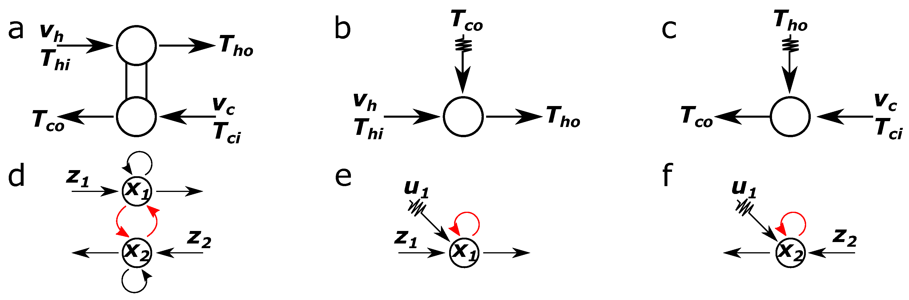
loopsLoops can reflect superfluous units.Loops appear when there are more units than necessary.Loops create strongly connected components that can be controlled (or observed) by only one driver (or sensor) node.
maximum matching [8]n/an/aUnmatched nodes provide driver and sensor nodes.
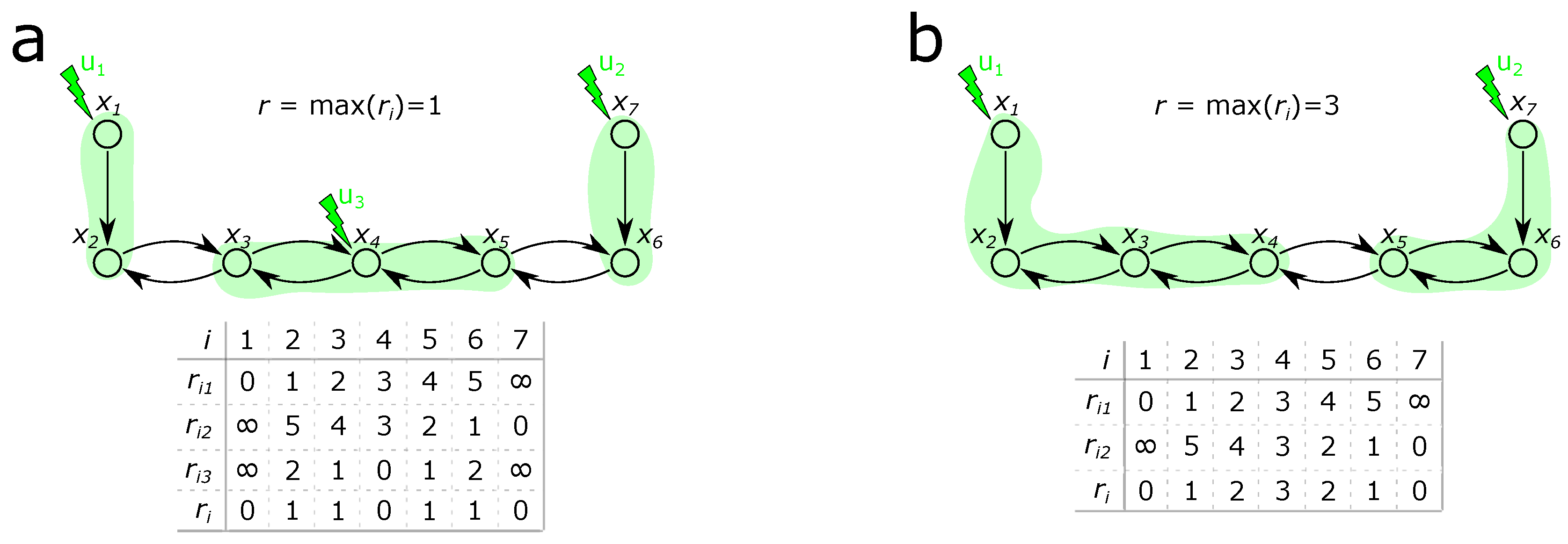
relative order [45]n/an/aDifficulty in operation.
number of components (S)Components are the disconnected sub-networks in the HEN.
Table 2. Structural properties of the SS, SM and DAE-based network representations of HENs.The operator | X | yields the cardinality of set X, and the operator X yields the average of the values in X.
PropertyCalculationSSSMDAE
number of nodes N = | V | Starting- and endpoints of the streams.Number of streams (Process and utility).Number of state variables necessary to describe the dynamics of HEN.
number of edges M = | E | Number of stream intervals.Number of units.Nonzero elements of the state-transition matrix.
degree k i o u t = j V A i j , k i i n = j V A j i , k i = k i o u t + k i i n Fixed for the nodes, k i = 1 for stream source and drains, k i = 2 for endpoints of stream intervals and k i = 4 for heat exchanger units. k i is the number of units on stream.Fixed for the nodes, k i moves from 2 to 4 in case of heat exchanger, and from 1 to 2 in case of utility units (loops are excluded).
shortest path i , j The minimum of length of paths from node i to node j.
distance matrixDThe distance matrix contains the shortest distance between node i and j , D i , j . The distance of node j is D i = j D i j .
cycle rank [53]LThe number of independent loops in the network.
total walk count (TWC) [54] T W C ( G ) = l = 1 N 1 i j A l The number of walks is proportional to the complexity, as the walks can represent the effect of an input signal in the system. More walks means more effect in the HEN.
coefficient of network complexity (CNC) [55] C N C ( G ) = M 2 / N Due to the fixed degree, the CNC is constrained.The proportion of units to streams.Due to the fixed degree, the CNC is constrained.
eccentricity [54] E c c ( i ) = max j V ( i , j )
E c c ( G ) = max i V ( E c c ( i ) )
Maximum length of heat loads.n/a.The relative order of the system.
Wiener index [56] W ( G ) = ( v , w ) E v , w Reflects the size of the HEN, and the complexity as long paths increase W ( G ) .In undirected case, W ( G ) should be divided by two. Since the network is undirected, W ( G ) approximates the size of the system.Longer geodesic paths represent higher order dynamics.
A/D index [54] A D ( G ) = k i / d i Since the degree is fixed, the index approximates the closeness of the units.As the order of heat exchanger units is not given, the A/D index does not necessarily characterise heat loads or HEN.Since degree is fixed, the index approximates the closeness of units.
Balaban-J index [57] B J ( G ) = M L + 1 ( v , w ) E D v D w Balaban-J index can only be calculated to undirected graphs.It approximates the size of the HEN.Balaban-J index can only be calculated to undirected graphs.
connectivity index [56] C I ( G ) = ( v , w ) E 1 / k v k w Since the degree is fixed, the index cannot characterise the HEN.Shows how the streams are interconnected.Since the degree is fixed, the index cannot characterise the HEN.
Table 3. Benchmark HENs and their optimisation methods that are used during the analysis. As the heuristic methods, CP, CRR, CSH, FLPR, GP, GSH, LFM, LHM, LHM-LP, LRR, SS, WFG and WFM were applied to each problem. This set of methods is denoted as HEU referring to heuristic methods. The methods are introduced in Table 4, where abbreviations are also presented.
ProblemHot StreamsCold StreamsMethodsSource
Furman and Sahinidis (2004)
4sp122HEU, BB [24]
6sp-cf133HEU, RET [18]
6sp-gg133HEU [64]
6sp133HEU, BB [24]
7sp-cm134HEU [65]
7sp-s161HEU [66]
7sp-torw143HEU [67]
7sp134HEU, SYN [25]
7sp233HEU, SYN [25]
7sp461HEU [68]
8sp-fs153HEU, E [69]
8sp144HEU [70]
9sp-al145HEU, E, MER, EC, ECR, ST [15]
9sp-has154HEU [71]
10sp-la145HEU [14]
10sp-ol146HEU [66]
10sp155HEU, BB [22]
12sp193HEU [70]
14sp177HEU [70]
15sp-tkm96HEU, E [72]
20sp11010HEU [70]
22sp-ph1111HEU [73]
22sp11111HEU [16]
23sp11112HEU, DS [17]
28sp-as11612HEU [74]
37sp-yfyv2116HEU, GASA [23]
Chen et al. (2015a,b)
balanced555HEU [61,62]
balanced888HEU [61,62]
balanced101010HEU [61,62]
balanced121212HEU [61,62]
balanced151515HEU [61,62]
unbalanced555HEU [61,62]
unbalanced101010HEU [61,62]
unbalanced151515HEU [61,62]
unbalanced171717HEU [61,62]
unbalanced202020HEU [61,62]
Grossmann (2017)
balanced12_random01212HEU [63]
balanced12_random11212HEU [63]
balanced12_random21212HEU [63]
balanced15_random01515HEU [63]
balanced15_random11515HEU [63]
balanced15_random21515HEU [63]
unbalanced17_random01717HEU [63]
unbalanced17_random11717HEU [63]
unbalanced17_random21717HEU [63]
unbalanced20_random02020HEU [63]
unbalanced20_random12020HEU [63]
unbalanced20_random22020HEU [63]
Table 4. Utilised methods and their objective functions.
NameMethodObjective FunctionSource
BBBranch and boundMinimises the heat exchanger and utility costs. [24]
CPCPLEX-solved transportation model.Minimum number of matches. [13]
CRRCovering Relaxation RoundingMinimum number of matches. [13]
CSHCPLEX-solved transshipment model.Minimum number of matches. [13]
DSDecomposition StrategyMinimises the number of exchangers. [17]
ENo method declaredExisting network, not optimised.
ECPinch methodologyEnergy-Capital cost minimisation. [14,15]
ECRPinch methodologyEnergy-Capital Retrofit cost minimisation. [14,15]
FLPRFractional LP RoundingMinimum number of matches. [13]
GASAGenetic Algorithm with Simulated AnnealingMinimises the annual cost. [23]
GPGurobi-solved transportation model.Minimum number of matches. [13]
GSHGurobi-solved transshipment model.Minimum number of matches. [13]
LFMLargest Fraction MatchMinimum number of matches. [13]
LHMLargest Heat Match GreedyMinimum number of matches. [13]
LHM-LPLargest Heat Match LP-basedMinimum number of matches. [13]
LRRLagrangian Relaxation RoundingMinimum number of matches. [13]
MERPinch methodologyMaximum Energy Recovery, Minimum Energy Requirement. [14,15]
RETStructural modifications by categoriesMinimises the cost of new exchangers, exchanger areas and piping. [18]
SSShortest StreamMinimum number of matches. [13]
STPinch methodologySupertargeting. [14,15]
SYNHeuristic stage-by-stage structuring synthesisMinimises the annual cost. [25]
WFGWater Filling GreedyMinimum number of matches. [13]
WFMWater Filling MILPMinimum number of matches. [13]
Table 5. Calculated measures and their short descriptions.
NameMeasureNetworkDescription
HEN-specific measures
numOfHotStream SMNum. of the hot streams in the problem.
numOfColdStream SMNum. of the hot streams in the problem.
hasPinch SS, DAETrue, if Pinch point is determined for the problem.
numOfExchangers SMNum. of heat exchanger cells in the designed HEN.
numOfUtilityHeater SMNum. of utility heater cells in the designed HEN.
numOfUtilityCooler SMNum. of utility cooler cells in the designed HEN.
numOfUnits U u n SMNum. of heat exchanger units in the designed HEN.
numOfMinUnits U m i n SMNum. of minimum units necessary for the problem.
Dynamical properties
numOfIndLoopLSMNum. of independent loops.
degOfFreedom SMDegree of freedom of heat loads.
numOfCompDAE DAENum. of sub-networks in the designed HEN.
numOfCompSMSSMNum. of components in the SM network.
numOfUMCon DAENum. of driver nodes granted by maximum matching.
numOfDriver DAENum. of actuator nodes necessary for controllability.
numOfUMObs DAENum. of sensor nodes granted by maximum matching.
numOfSensor DAENum. of sensor nodes necessary for observability.
sluggishnessrDAERelative order of the HEN.
targetOrder r m a x DAETarget relative order (in our case: d m a x / 4 ).
actCovSize DAENum. of actuators determined by the set-covering method.
senCovSize DAENum. of sensors determined by the set-covering method.
actCovRetSize DAENum. of actuators determined by the retrofit set-covering method.
senCovRetSize DAENum. of sensors determined by the retrofit set-covering method.
actNetMesSizeRet DAENum. of actuators determined by the retrofit centrality-based method.
senNetMesSizeRet DAENum. of sensors determined by the retrofit centrality-based method.
Network-based structural properties
balabanJIndex B J ( G ) SMBalaban-J index of the SM network.
numOfNodes.ofDAENDAENum. of nodes in the DAE network.
numOfNodes.ofSMNSMNum. of nodes in the SM network.
numOfNodes.ofSSNSSNum. of nodes in the SS network.
numOfEdges.ofDAEMDAENum. of edges in the DAE network.
numOfEdges.ofSMMSMNum. of edges in the SM network.
numOfEdges.ofSSMSSNum. of edges in the SS network.
averageDegree.ofDAE k i DAEAverage degree in the DAE network.
averageDegree.ofSM k i SMAverage degree in the SM network.
averageDegree.ofSS k i SSAverage degree in the SS network.
eccentricity.ofDAE E c c ( G ) DAEGraph eccentricity value of DAE network.
eccentricity.ofSM E c c ( G ) SMGraph eccentricity value of SM network.
eccentricity.ofSS E c c ( G ) SSGraph eccentricity value of SS network.
totalWalkCount.ofDAE T W C ( G ) DAENum. of walks in the DAE network.
totalWalkCount.ofSM T W C ( G ) SMNum. of walks in the SM network.
totalWalkCount.ofSS T W C ( G ) SSNum. of walks in the SS network.
coeffNetwCompl.ofDAE C N C ( G ) DAECoefficient of network complexity in the DAE network.
coeffNetwCompl.ofSM C N C ( G ) SMCoefficient of network complexity in the SM network.
coeffNetwCompl.ofSS C N C ( G ) SSCoefficient of network complexity in the SS network.
adIndex.ofDAE A D ( G ) DAEA/D index of the DAE network.
adIndex.ofSM A D ( G ) SMA/D index of the SM network.
adIndex.ofSS A D ( G ) SSA/D index of the SS network.
wienerIndex.ofDAE W ( G ) DAEWiener index of the DAE network.
wienerIndex.ofSM W ( G ) SMWiener index of the SM network.
wienerIndex.ofSS W ( G ) SSWiener index of the SS network.
connInd.ofDAE.inConn C J ( G ) DAEConnectivity index for in-degree in DAE network.
connInd.ofDAE.outConn C J ( G ) DAEConnectivity index for out-degree in DAE network.
connInd.ofSM C J ( G ) SMConnectivity index for SM network.
connInd.ofSS.inConn C J ( G ) SSConnectivity index for in-degree in the SS network.
connInd.ofSS.inConn C J ( G ) SSConnectivity index for out-degree in the SS network.
Table 6. Calculated measures and their short descriptions.
Name9sp-al1 - E9sp-al1 - MER9sp-al1 - EC9sp-al1 - ECR
HEN-specific measures
numOfHotStream4444
numOfColdStream5555
hasPinch0100
numOfExchangers512108
numOfUtilityHeater2222
numOfUtilityCooler3333
numOfUnits10171513
numOfMinUnits10101010
Dynamical properties
numOfIndLoop0753
degOfFreedom−520−2
numOfCompDAE4111
numOfCompSM1111
numOfUMCon0000
numOfDriver4111
numOfUMObs0000
numOfSensor5555
sluggishness29811
targetOrder1322
actCovSize9787
senCovSize5464
actCovRetSize9777
senCovRetSize7465
actNetMesSizeRet98108
senNetMesSizeRet7477
Network-based structural properties
balabanJIndex9.92124.39905.62345.2789
numOfNodesofDAE15292521
numOfNodesofSM11111111
numOfNodesofSS721079787
numOfEdgesofDAE31736149
numOfEdgesofSM10171513
numOfEdgesofSS7111310189
averageDegreeofDAE2.13333.03452.88002.6667
averageDegreeofSM1.81823.09092.72732.3636
averageDegreeofSS1.97222.11212.08252.0460
eccentricityofDAE3121111
eccentricityofSM7545
eccentricityofSS13282225
totalWalkCountofDAE802,7881.02127E+1392,080,948,1861,364,370,909
totalWalkCountofSM34,2582,114,4902,114,490410,032
totalWalkCountofSS646913832741977
coeffNetwComplofDAE64.0667183.7586148.8400114.3333
coeffNetwComplofSM9.090926.272720.454515.3636
coeffNetwComplofSS70.0139119.3364105.164991.0460
adIndexofDAE0.84210.05220.06610.0787
adIndexofSM0.11360.26360.25860.1857
adIndexofSS0.04460.00670.00890.0107
wienerIndexofDAE3816871090712
wienerIndexofSM176129116140
wienerIndexofSS3,18133,52422,58616,582
connIndofDAEIn0.01540.00530.00650.0085
connIndofDAEOut0.01470.00520.00630.0082
connIndofSS0.02460.00820.01030.0143
connIndofSMIn0.01310.00770.00870.0100
connIndofSMOut0.01310.00770.00870.0100

